Finite temperature $SU(2)$ gauge theory: critical coupling and universality class

Abstract

We examine $SU(2)$ gauge theory in $3+1$ dimensions at finite temperature in the vicinity of critical point. For various lattice sizes in time direction ($N_{\tau}=1,2,4,8$) we extract high precision values of the inverse critical coupling and critical values of the 4-th order cumulant of Polyakov loops (Binder cumulant). We check the universality class of the theory by comparing the cumulant values to that of the $3D$ Ising model and find very good agreement.

The Polyakov loop correlators for the indicated lattices are also measured and the string tension values extracted. The high precision values of critical coupling and string tension allow us to study the scaling of dimensionless $T_{c}/\sqrt{\sigma}$ ratio. The violation of scaling by $<10\%$ is observed as the coupling is varied from weak to strong coupling regime.

1 Introduction

The original motivation for this study was to re-derive the values of critical coupling for finite temperature $SU(2)$ gauge theory formulated on lattices with different time-like extent $N_{\tau}$ at the highest precision possible with modern computational resources (we utilize a small 20-30 node computer cluster). For this we rely on the property of universality of $SU(2)$ gauge theory at the second order critical point. We adopt a standard for such models procedure of locating the position of critical point, which amounts to measuring the 4th order (Binder) cumulant[1] $g_{4}$ for Polyakov loops $P$

$$g_{4}=1-\frac{\langle P^{4}\rangle}{3\langle P^{2}\rangle^{2}},\quad P=\frac{1}{N_{\sigma}^{3}}\sum_{\vec{x}}\frac{1}{2}{\rm Tr}\prod_{\tau=1}^{N_{\tau}}U_{\tau,\vec{x};0}$$ (1)

on $N_{\tau}\times N_{\sigma}^{3}$ lattices in the vicinity of phase transition. Note that we use the original form of the Binder cumulant which differs by a constant factor $1/3$ from the normalized version frequently used in lattice gauge theory literature. The finite size scaling (FSS) of $g_{4}$ with lattice size $N_{\sigma}$ in the vicinity of the critical point is known[2, 3]

$$g_{4,N_{\sigma}}\approx g_{4,\infty}(1+a_{1}tN_{\sigma}^{1/\nu}+a_{2}N_{\sigma}^{-y_{1}}+\cdots)$$ (2)

where $t=(T-T_{c,\infty})/T_{c,\infty}$ is the reduced temperature and $y_{1}\equiv-\omega>0$ is the exponent of the largest irrelevant scaling field.

The scaling of the temperature value of the intersection point of Binder cumulant curves $g_{4}(t)$ on $N_{\sigma}$ and $N^{\prime}_{\sigma}=bN_{\sigma},\,b>1$ lattices is

$$t^{*}=-\frac{a_{2}}{a_{1}}N_{\sigma}^{-y_{1}-1/\nu}\frac{1-b^{-y_{1}}}{1-b^{1/\nu}}.$$ (3)

It is convenient to define $L_{b}=N_{\sigma}^{-y_{1}-1/\nu}(1-b^{-y_{1}})/(1-b^{1/\nu})$, so that (3) becomes a simple linear function of $L_{b}$. Substituting $t^{*}$ into (2) results in the scaling for the intersection $g_{4}$ value

$$g^{*}_{4}=g_{4,\infty}\left(1+a_{2}N_{\sigma}^{-y_{1}}\frac{1-b^{-y_{1}-1/\nu}}{1-b^{-1/\nu}}\right).$$ (4)

Here we define $L_{g}=N_{\sigma}^{-y_{1}}(1-b^{-y_{1}-1/\nu})/(1-b^{-1/\nu})$, so that (4) is linear in $L_{g}$.

The well-known renormalization group relationship allows us to connect the lattice spacing to the coupling $\beta=2N_{c}/g^{2}$, ($N_{c}=2$)

$$a\Lambda_{N_{\sigma}}=\left(\frac{\beta}{2N_{c}b_{0}}\right)^{b_{1}/2b_{0}^{2}}\exp\left(-\frac{\beta}{4N_{c}b_{0}}\right).$$ (5)

Using the fact that the temperature is $T=1/(N_{\tau}a)$ one obtains the following expression for the reduced temperature in the vicinity of the transition point

$$t=\frac{\beta-\beta_{c,\infty}}{4N_{c}b_{0}}\left(1-\frac{2N_{c}b_{1}}{b_{0}}\beta^{-1}_{c,\infty}\right)+O((\beta-\beta_{c,\infty})^{2}).$$ (6)

In the studies of $N_{\tau}=8$ and 16 phase transitions by Fingberg et al.[4] no deviations from the leading term were found. Therefore one can assume linear correspondence between the reduced temperature and reduced inverse coupling and perform the scaling studies in terms of the inverse lattice coupling $\beta$.

In their renowned work Svetitsky and Yaffe[5] conjectured that the universality class of the $d+1$-dimensional $SU(2)$ gauge theory is the $d$-dimensional Ising model. Since then it was confirmed in numerous numerical simulations, e.g. Ref. [6] for $N_{\tau}=4$ theory. Indeed, we observe that for all lattices in the thermodynamic limit the $g_{4}$ curves intersect in the vicinity of the $3D$ Ising value, albeit with different degree of accuracy.

In section 2 we measure values of Binder cumulant in the vicinity of the critical point and determine critical values of inverse coupling and Binder cumulant for $N_{\tau}=1,2,4,8$ lattices. Our treatment of different $N_{\tau}$ lattices is not uniform. We conduct the FSS study for $N_{\tau}=4$ and 2 lattices, while relatively large $N_{\sigma}$ values used for $N_{\tau}=1$ studies prevented us from observing a significant scaling behavior. The $N_{\tau}=8$ lattice allows for the FSS study, however it is very expensive to simulate and therefore is studied assuming the Ising universality class.

The small $N_{\tau}=1$ and 2 lattices are of special interest in decimation studies, since the iterative block-spinning procedure has to be stopped when the smallest (or next to smallest) lattice is reached. Therefore for $N_{\tau}=1$ lattice we consider a specific lattice formulation suitable for decimation.

In section 3 we study the quark-antiquark static potential and extract the string tension for $N_{\tau}/3\geq 2$ lattices at temperature $T=T_{c}/3$. The knowledge of critical couplings allows us to construct the dimensionless ratio $T_{c}/\sqrt{\sigma}$ and study its scaling with coupling. We observe relatively small $<10\%$ violation of scaling at strong coupling $\beta=1.8738$ value.

2 Finite temperature phase transition: Monte Carlo study

In all simulations performed in this study we use the standard Wilson action. Per one updating sweep we perform two overrelaxation steps and one heatbath update. We use a standard acceptance improved heat bath updating procedure[7, 8]. Measurements are performed every $2-20$ sweep. We use $10-80$ independent runs (at different initial random generator seeds), each run is averaged into a single bin. This allows us to gain better statistics and avoid autocorrelations. All errors are computed with the jack-knife method with respect to these bins, except when indicated differently. For various coupling values $\beta=4/g^{2}$ in the visinity of the finite temperature confinement-deconfinement phase transition after initial equilibration we measure Polyakov loops and compute the Binder cumulant. The number of sweeps needed for the system to reach equilibrium is estimated by observing the Monte Carlo time evolution of the Polyakov loop and plaquette estimates for each of the lattice sizes and typical equilibration times are $\geq 10^{3}$ sweeps.

2.1 $N_{\tau}=4$ lattice

We start with perhaps the most studied lattice $N_{\tau}=4$. At this point we do not need to assume any particular universality class. We simulate $N_{\sigma}=8,10,16,20,24$ and $32$ lattices, with typical statistics of $30\times 40000$ configurations.

Figure 1: The Binder cumulant $g_{4}$ for $N_{\tau}=4$, $N_{\sigma}=8,10,16,24,32$ lattices. Linear fits are represented by solid lines, the $T_{c}$ estimate with errors by vertical lines.

$N_{\sigma}$	8	10	16	20	24	32
$a$	4.17(29)	5.77(36)	11.80(56)	17.6(1.2)	20.6(1.3)	34.7(1.9)
$b$	-9.13(66)	-12.89(82)	-26.7(1.3)	-39.9(2.8)	-46.9(2.0)	-79.3(4.3)

Table 1: Resulting parameters of the $\chi^{2}$ fit of the Binder cumulant to a linear $g_{4}(\beta)=a\beta+b$ function.

Figure 2: The rescaled Binder cumulant $g_{4}(N_{\sigma}^{1/\nu}(\beta-\beta_{c})/\beta_{c})$ for $N_{\tau}=4$, $N_{\sigma}=8,10,16,24,32$ lattices.

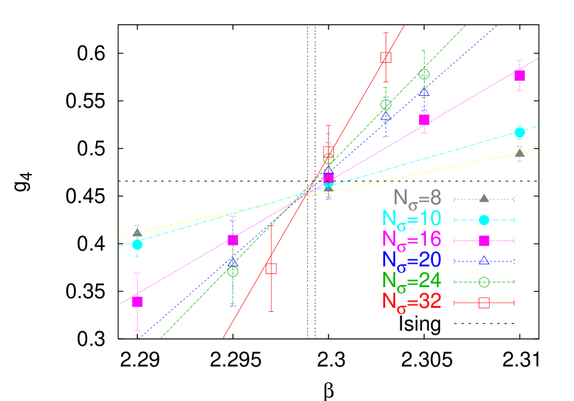
The results for the Binder cumulant measurement are presented in Fig. 1 together with the fitting lines $g_{4}(\beta)=a\beta+b$ (see Tab. 1 for fitting parameters).

$N_{\sigma}$	8	10	16	20	24
10	2.2960(19)	*	*	*	*
16	2.2985(40)	2.2992(5)	*	*	*
20	2.2985(44)	2.2988(5)	2.2984(12)	*	*
24	2.2983(28)	2.2986(3)	2.2981(7)	2.2977(29)	*
32	2.2987(11)	2.2989(1)	2.2988(2)	2.2990(4)	2.2993(3)
10	0.4370(87)	*	*	*	*
16	0.4476(19)	0.4556(41)	*	*	*
20	0.4474(20)	0.4533(38)	0.446(15)	*	*
24	0.4468(14)	0.4520(31)	0.4433(99)	0.433(56)	*
32	0.4486(08)	0.4540(22)	0.4514(46)	0.457(11)	0.466(9)

Table 2: Pairwise intersection coordinates in $g_{4}-\beta$ plane: the inverse lattice coupling (top) and the 4th cumulant (bottom); $N_{\tau}=4$.

The data is fitted to a straight line in the vicinity of the transition point with a standard $\chi^{2}$ procedure. The errors in the fitting parameters $a$ and $b$ are obtained by error propagation. The resulting goodness of fit in all cases is $Q\approx 0.6-0.9$, which confirms that at the considered $\beta$ values the $g_{4}$ curves are well approximated by lines. In Tab. 2 we list the values $\beta^{*}$ and $g_{4}^{*}$ of intersection points for different pairs of lines ($N_{\sigma}$, $N^{\prime}_{\sigma}=bN_{\sigma}$).

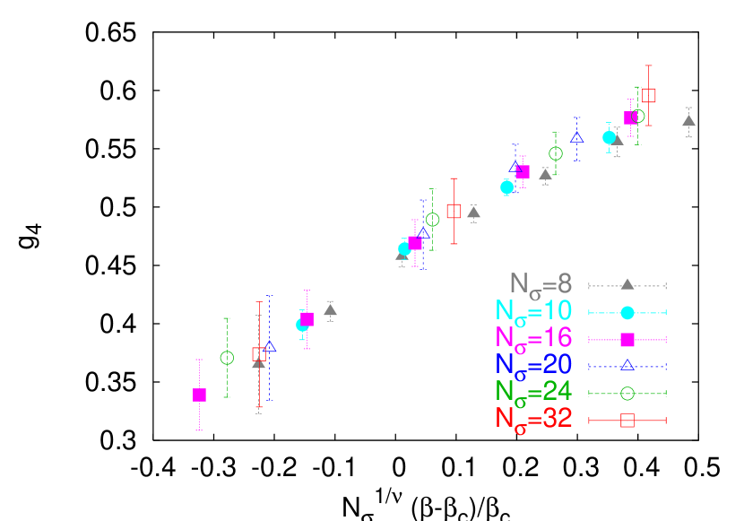
First we check the assumed scaling behavior by plotting the rescaled Binder cumulant $g_{4}(N_{\sigma}^{1/\nu}(\beta-\beta_{c})/\beta_{c})$ for various lattice sizes, see Fig. 2. For the critical coupling value we use $\beta_{c}=2.2991$, which we will obtain later in the FSS study. Indeed, we observe that the curves fall on top of each other. The only noticeable deviation from the scaling behavior can be observed for the smallest considered lattice $N_{\sigma}=8$ far away from the transition point. This is obviously due to the effects from next to leading order scaling terms. The important observation is that in the region where we perform linear fits there is no deviation from the scaling for all the lattices and also apparently the linearity holds.

Next we study the scaling of the pair-wise intersection point coordinates according to (3) and (4). First we look at the $\beta^{*}$ coordinate of intersection points versus $L_{b}$, see Fig. 3, and then at the $g^{*}_{4}$ coordinte of intersection points versus $L_{g}$, see Fig. 4. For this we need to know the values of critical exponents $\nu$ and $y_{1}$. As we will see (from the quality of data) it is not practical to extract them from the data, instead we take them to be equal to the Ising values known with good accuracy $1/\nu=1.5887(85)$ and $y_{1}=0.812$ [9]. For a self-consistency check we verify that the scaling resulting from use of these values is adequate.

For each smaller lattice size from $N_{\sigma}=10,16,20,24$ set (represented by a different point type/color on the figure) we take various possible $b$ values, which index the larger lattice.

Figure 3: The $\beta^{*}$ coordinates of the pair-wise intersection points for $N_{\sigma}\equiv L=10,16,20,24$ and various $b$ lattices. The solid line represents a linear fit for all the presented data. $N_{\tau}=4$.

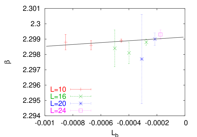
As one can see from Fig. 3 despite the fact that the simulation statistics is sufficient for the precise location of the intersection point the error bars can become large as intersecting lines approach the collinear limit. We performed a linear fit in accordance with (3). The goodness of fit is $Q=0.66$ which suggests that the scaling equation is correct. The limit $L_{b}\rightarrow 0$ corresponds to the thermodynamic limit and yields $\beta_{c,\infty}=2.2991(2)$. Note that the largest lattices intersection ($N_{\tau}=24$ and $N_{\tau}^{\prime}=32$) happens at $\beta^{*}=2.2993(3)$ which agrees with the thermodynamic limit result. These results should be compared with the value $\beta_{c}=2.2985(6)$ of Ref. [6] or $2.2986(6)$ (intersection 12 and 18) of Ref. [10] and indeed we find a very good agreement.

Figure 4: Same as Fig. 3, but for the Binder cumulant. The horizontal line is the Ising $g_{4}^{Ising}=0.46575$ value.

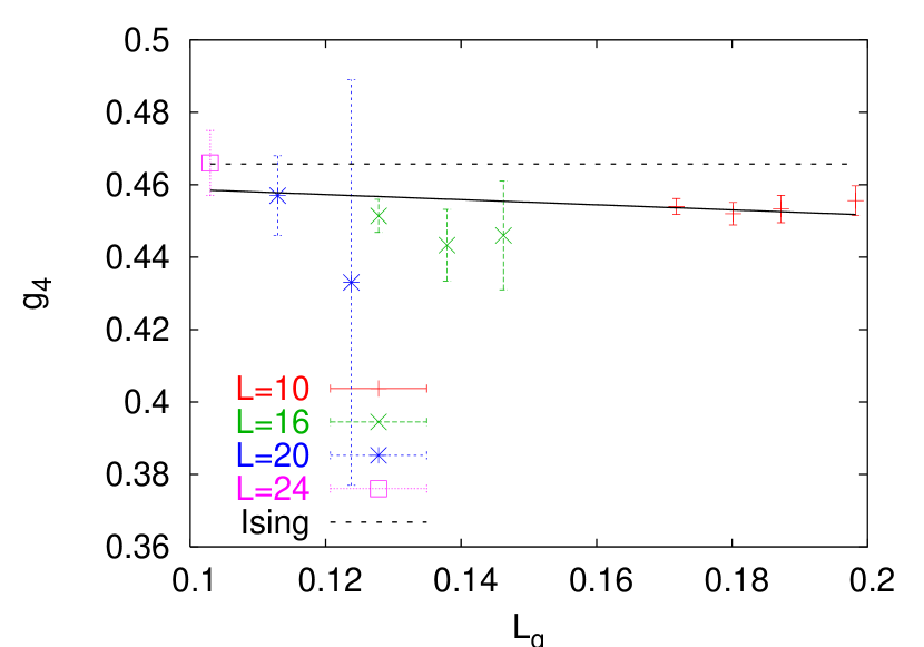
The value of Binder cumulant for the 3D Ising model is well known. In the lattice gauge theory literature the early estimate of Ferrenberg et al. $g_{4}^{Ising}=0.470(5)$ [9] is often used. In this work we are using the more recent and more accurate estimate of Hasenbusch et al. [11] $Q\equiv<m^{2}>^{2}/<m^{4}>=0.62393(13)$ (here $m$ is the Ising model magnetization), which translates into $g_{4}^{Ising}=0.46575(11)$.

The data of Tab. 2 and Fig. 1 strongly support the fact that the Binder cumulant reaches the Ising value for the larger lattice intersections. Therefore it is safe to assume that within the accuracy of this study the $N_{\tau}=4$ model is indeed in the 3D Ising model universality class.

We continue the study of the scaling of pair-wise intersection point coordinates with the size of participating lattices. Now similarly to $\beta^{*}$ analysis we plot the $g_{4}^{*}$ values of intersection points versus $L_{g}$, see Fig. 4. As one can see the data does not allow to perform a quality fit especially in the thermodynamic limit $L_{g}\rightarrow 0$. Since we already assumed that the Ising universality class holds we may fit $g_{4}$ directly to $a*\beta+g_{4}^{Ising}$. The reduction of the degrees of freedom allows for a better defined fit. The goodness of fit is $Q=0.80$ meaning that the scaling function is plausible. Also it represents a self-consistency check for the assumption of the Ising universality class.

At this point it is worth to mention that in the studies of the Dyson’s hierarchical model [12] it was observed that a too coarse scale in the $\beta$ sampling may lead to inaccurate locations of the intersections when linear fits are used. This inaccuracy may generate sizable errors in the $L_{b}\rightarrow 0$ and $L_{g}\rightarrow 0$ limits.

As a side note we would like to point that insufficient statistics prevented us from performing the fits inside separate bins and thus obtaining the relevant errors by use of the jack-knife method on this bins. Instead the fits were performed on a whole set and the errors were obtained by simple error propagation, which may undermine their accuracy.

2.2 $N_{\tau}=2$ lattice

Next we study $N_{t}=2$ lattice. This lattice is somewhat special because unlike larger $N_{\tau}$ lattices as a result of periodic boundary conditions in $T$ direction every pair of spatial links from different time slices is connected only by a single time-like link.

$N_{\sigma}$	10	16	24
16	1.87331(2)	*	*
24	1.87338(1)	1.87343(2)	*
32	1.873422(5)	1.87345(1)	1.87348(2)
16	0.4558(3)	*	*
24	0.4565(2)	0.4578(4)	*
32	0.4568(1)	0.4583(2)	0.4595(10)

Table 3: Pairwise intersection coordinates in $g_{4}-\beta$ plane: the inverse lattice coupling (top) and the 4th cumulant (bottom); $N_{\tau}=2$.

Figure 5: The Binder cumulant $g_{4}$ for $N_{\tau}=2$, $N_{\sigma}=10,16,24,32$ lattices. Linear fits are represented by solid lines, the $T_{c}$ estimate with errors by vertical lines.

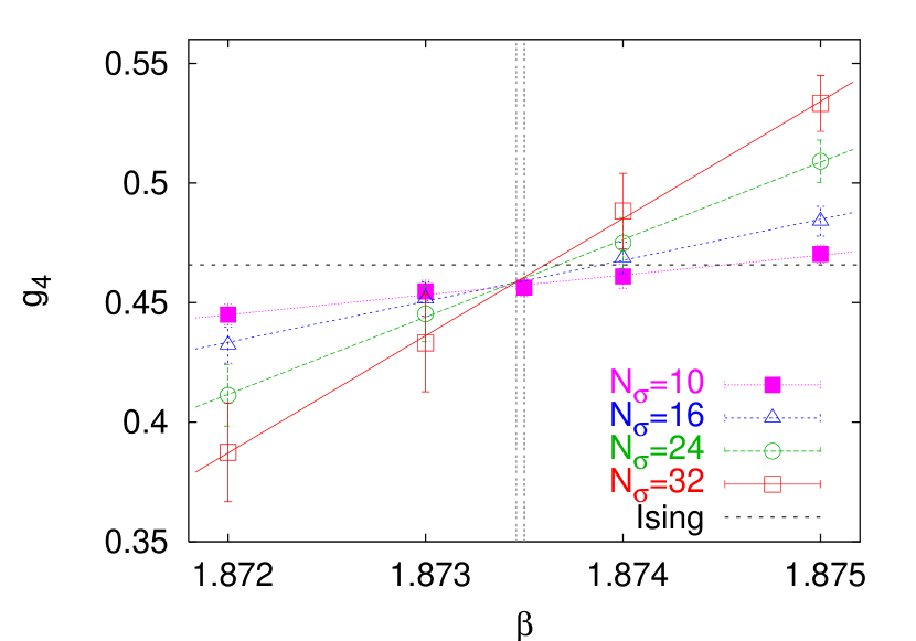
For this lattice we generated on average from $10\times 0.5*10^{5}$ configurations for $N_{\sigma}=16$ to $10\times 0.3*10^{5}$ configurations for $N_{\sigma}=32$ lattices. The results for Binder cumulant measurements in the vicinity of transition point are presented in Fig. 5. As one can see from the figure the linear fit lines intersect clearly below the Ising value and at what appears to be a single point. We collect the coordinates of the intersection points of the fitting lines in Tab. 3. We observe that for the intersection coordinate $\beta^{*}$ of larger lattices there is very insignificant scaling change. Therefore for this quantity we do not perform the FSS analysis and take as the transition coupling the value of intersection of lines of the largest 32 and 24 lattices: $\beta_{c}=1.87348(2)$.

Figure 6: Same as Fig. 4, but for $N_{\tau}=2$ lattice.

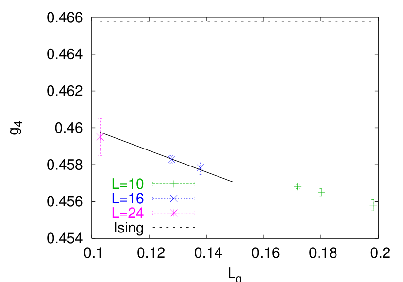
For the other intersection coordinate $g_{4}^{*}$ there is a noticeable scaling behavior, therefore we perform the FSS analysis analogous to the presented earlier ($N_{\tau}=4$). The results are plotted in Fig. 6. It is interesting that the smaller $N_{\sigma}=10$ lattice is not consistent with the scaling behavior, while it was for $N_{\tau}=4$ lattice. This can indicate that the sub-leading effects can be stronger here. For the larger lattices, however, the fit is good and indicates that the assumed $3D$ Ising universality class is correct. Also the assumption of the $3D$ Ising universality class is suported by independent studies of critical exponent $\nu$ [13].

It is expected that for lattices with smaller $N_{\tau}$ it is sufficient to consider lattices with correspondingly smaller $N_{\sigma}$ values, therefore it is surprising that the intersection point of $N_{\sigma}=32$ and 24 lattices is located statistically significantly below the Ising $g^{Ising}_{4}$ value and one needs even larger lattices to reach the value corresponding to the thermodynamic limit.

For $N_{\tau}=2$ we found several estimates in the most recent literature all in good agreement with our result. On $2\times 12^{3}$ lattice the estimate is $\beta_{c}=1.877$ (no error given, presumably $1.877(1)$) [14], while more recent estimate from $2\times 30^{3}$ and $2\times 40^{3}$ lattices gives $\beta_{c}=1.8735(4)$ [15, 16].

2.3 $N_{\tau}=1$ lattice

Here we look at even more exceptional $N_{\tau}=1$ lattice. This lattice is very special and allows for two formulations. One formulation is motivated by considering the sum over plaquettes in the partition function. It is natural to assume that there is one time-like plaquette for each space coordinate. This case requires special treatment of space-like links since they have conjugate staples only in one time direction (we choose positive direction) unlike two directions (positive and negative) for other directions. The other formulation can be motivated by considering the $N_{\tau}=2$ lattice and performing factor 2 decimation in time direction (removing one time slice of links). In this formulation there is no special treatment of conjugate staples of space-like links. One has to consider staples in both positive and negative direction for each direction (including the time direction).

We start with the first formulation of $N_{\tau}=1$ lattice, which we call time-like plaquette single counting. Afterwards we will consider the second formulation which we refer to as time-like plaquette double counting.

For single counting formulation we present the results in Fig. 7.

Figure 7: The Binder cumulant $g_{4}$ for $N_{\tau}=1$ (single counting), $N_{\sigma}=8,16,24,32$ lattices. Linear fits are represented by solid lines, the $T_{c}$ estimate with errors by vertical lines.

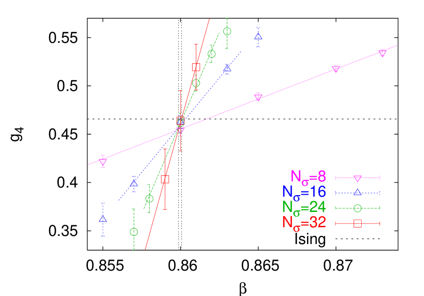
Similarly to $N_{\tau}=2$ case we do not observe any scaling behavior since the lines cross at a single point. The linear fitting lines intersection coordinates are:

$$N_{\sigma}=8,N_{\sigma}^{\prime}=16 - \beta^{*}=0.85969(13),g^{*}_{4}=0.4535(20),$$

$$N_{\sigma}=16,N_{\sigma}^{\prime}=24 - \beta^{*}=0.85989(11),g^{*}_{4}=0.4573(28),$$

$$N_{\sigma}=24,N_{\sigma}^{\prime}=32 - \beta^{*}=0.85997(10),g^{*}_{4}=0.4606(51).$$

Note little change in the $\beta^{*}$ and $g^{*}_{4}$ coordinates, there is virtually no scaling to be extracted here. The intersection of the largest lattices (32 and 24) defines the critical coupling $\beta_{c}=0.85997(10)$. The Binder cumulant is within one sigma from the Ising value.

Next we study the second formulation with time-like plaquettes double counting. We summarize the results in Fig. 8. The pairwise fitting lines intersection coordinates in this case are:

$$N_{\sigma}=8,N_{\sigma}^{\prime}=16 - \beta^{*}=0.86198(11),g^{*}_{4}=0.4549(22),$$

$$N_{\sigma}=16,N_{\sigma}^{\prime}=24 - \beta^{*}=0.86228(6),g^{*}_{4}=0.4606(12),$$

$$N_{\sigma}=24,N_{\sigma}^{\prime}=32 - \beta^{*}=0.86226(6),g^{*}_{4}=0.4598(31).$$

Figure 8: The Binder cumulant $g_{4}$ for $N_{\tau}=1$ (double counting), $N_{\sigma}=8,16,24,32$ lattices. Linear fits are represented by solid lines, the $T_{c}$ estimate with errors by vertical lines.

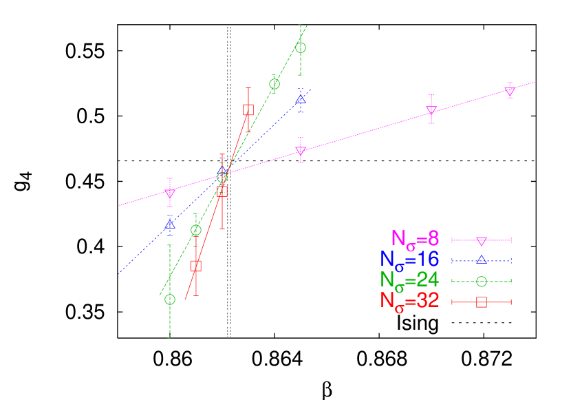
Again there is almost no scaling behavior in the coordinates. The values of Binder cumulant are comparable to the previous formulation, however the inverse critical coupling is shifted toward larger values. Also we observe that the Binder cumulant deviation from the Ising value is small ($<2\sigma$ away).

The only known result in the recent literature for $N_{\tau}=1$ lattice is $\beta_{c}=0.8730(2)$ [17]. However, the authors do not indicate how it was obtained.

2.4 $N_{\tau}=8$ lattice

Next we look at $N_{\tau}=8$ and $N_{\sigma}=16,24$ and $32$ lattices. We present the results in Fig. 9. For lattice $N_{\sigma}=16$ we performed $10^{6}$ sweeps, while for $N_{\sigma}=24$ and $32$ lattices we performed $0.2\times 10^{6}$ sweeps (measuring every 20) at the three beta values closest to the transition.

The approach adopted for smaller lattices is not very efficient here. The fitting lines for larger two lattices intersect at

$$N_{\sigma}=24,N_{\sigma}^{\prime}=32 - \beta=2.5113(19),g_{4}=0.472(13).$$

As one can see the errors are quite significant here and better statistics is needed.

Figure 9: The Binder cumulant $g_{4}$ for $N_{\tau}=8$, $N_{\sigma}=16,24,32$ lattices. Linear fits are represented by solid lines, the $T_{c}$ estimate with errors by vertical lines.

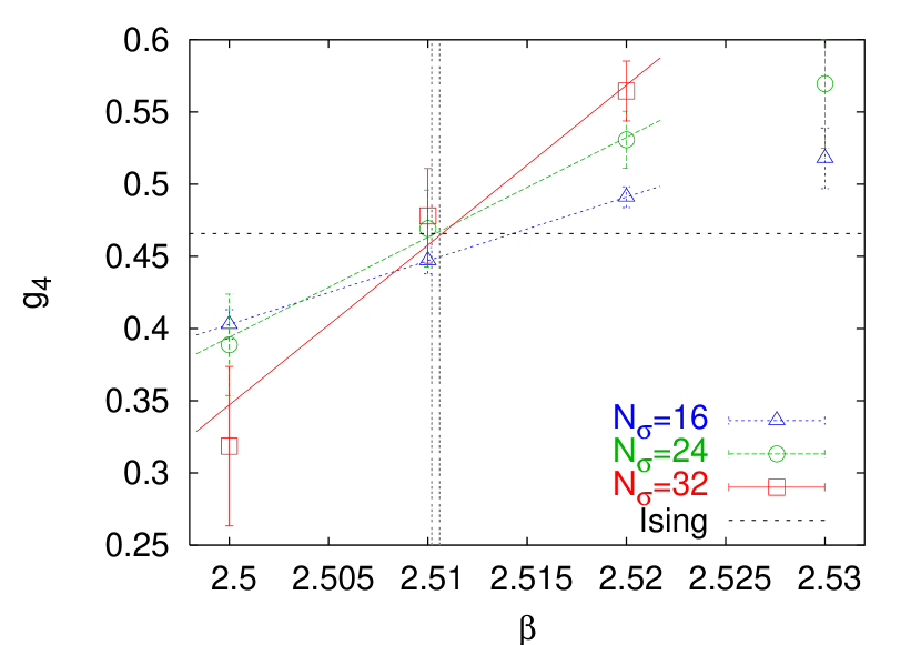
On the other hand if one assumes the universallity class of the $3D$ Ising model it is possible to obtain better results. Our strategy is similar to one used in Ref. [18]. We look at the points of intersection of linear fitting curves with the $3D$ Ising Binder cumulant value

$$N_{\sigma}=16 \beta=2.5143(0)$$

$$N_{\sigma}=24 \beta=2.5104(2)$$

$$N_{\sigma}=32 \beta=2.5107(8).$$

The crossing of the fitting line with the Ising value defines the transition point. Note that $N_{\sigma}=16$ lattice intersects with $N_{\sigma}=24$ slightly off, while $N_{\sigma}=24$ and $N_{\sigma}=32$ at the Ising value. This indicates that the thermodynamic limit has set in for $N_{\sigma}\geq 24$. The uncertainties of the fitting parameters contribute to the error of the critical coupling. Possibly the best result is for $N_{\sigma}=24$ lattice since the larger lattice is a bit noisier, therefore we define $\beta_{c}=2.5104(2)$.

We compare our result to a similarly performed study of Ref. [18], which is $\beta_{c}=2.5105(10)$ for $N_{\tau}=8$ and $N_{\sigma}=32,40,48$ lattices. The Gaussian difference test yields $Q=0.92$, indicating good correspondence of the results.

3 String tension and physical scale

In the previous section by measuring the critical Binder cumulant value we obtained high precision critical coupling values for various $N_{\tau}$ lattices. In this section we measure the Polyakov loop correlator and correspondingly obtain the static quark-antiquark potential. The results of the previous section make possible to study the scaling of dimensionless ratio $T_{c}/\sqrt{\sigma}$ well into the strong coupling regime ($\beta=1.87380$).

To fix the scale we use the critical coupling estimates of the previous section together with the value from the literature [18] for $N_{\tau}=12$ lattice. The critical temperature $T_{c}=1/(N^{c}_{\tau}*a)$ fixes the lattice spacing in physical units. The lattice is then simulated at these $\beta_{c}$ values but at different $N_{\tau}=3\cdot N^{c}_{\tau}$ corresponding to $T=T_{c}/3$. At this temperature finite temperature correction should be minimal.

For the string tension measurements we use Lüscher-Weisz multilevel algorithm [19, 20]. As was noted in the second reference the one level algorithm is computationally preferable. In our simulations the lattice is sliced into layers of thickness $2a$. On each layer we perform 10 sweeps for $N_{\tau}/3=12$ lattice, 100 sweeps for $N_{\tau}/3=8$ lattices, and 1000 sweeps for $N_{\tau}/3=4$ and 2 lattices.

We fit the potential using the following ansatz

$$\hat{V}(\hat{r})=\hat{V}_{0}-\frac{\hat{\mu}}{\hat{r}}+\hat{\sigma}\hat{r},$$ (7)

where the hats indicate lattice dimensionless observables.

The fit of the potential is performed in the range $\hat{r}\in[2,5-9]$, which ensures that no short distance $O(1/r^{3})$ or long distance (reduced signal/noise or effects from propagation across the periodic boundary condition) artifacts contribute.

$N_{\tau}/3$	$\beta$	$\hat{V}_{0}$	$\hat{\mu}$	$\hat{\sigma}$	$T_{c}/\sqrt{\sigma}$
12	2.6355(10)	0.524(28)	0.273(35)	0.0153(53)	0.67(12)
8	2.51098(58)	0.5505(10)	0.2757(12)	0.03232(18)	0.6953(19)
4	2.29850(6)	0.5826(6)	0.3241(7)	0.13312(10)	0.6852(03)
2	1.87380(3)	0.313(13)	0.256(15)	0.6285(26)	0.6307(13)

Table 4: The parameters of the potential fit in lattice units and the string tension in (physical) units of $T_{c}$ for various $N_{\tau}/3\equiv N_{\tau}^{c}$ lattices.

In table 4 we collect the data from the potential fits to the ansatz (7). The typical goodness of fit $Q\in[0.42,0.99]$. Note that for $N_{\tau}/3=2,4,8$ lattices we performed the simulations at $\beta$ values from our earlier estimates, which are slightly different from the final values presented in the previous section. For the errors on the inverse coupling we take either the difference to the final value or the final value error, depending on which one is larger.

In order to compare the string tension $\hat{\sigma}$ obtained on different lattices, we need to convert the lattice observable to physical units. The string tension in physical units is $\sigma=\hat{\sigma}/a^{2}$. We can express the lattice spacing in physical units through the critical temperature $a=1/(T_{c}\cdot N_{\tau}^{c})$. Therefore we can construct a dimensionless observable $T_{c}/\sqrt{\sigma}=(N_{\tau}^{c}\cdot\sqrt{\hat{\sigma}})^{-1}$, which we present in the last column of the table. The uncertainties come from the estimates of $a$ and the string tension $\hat{\sigma}$

$$\frac{T_{c}}{\sqrt{\sigma}}=\frac{T_{c}a}{\sqrt{\hat{\sigma}}}.$$ (8)

Therefore the error of this observable is

$$\delta(\frac{T_{c}}{\sqrt{\sigma}})=\left(\left(\frac{1}{8N_{\tau}^{c}b_{0}}\delta\beta_{c}\right)^{2}+\left(\frac{1}{2N_{\tau}^{c}\hat{\sigma}^{3/2}}\delta\hat{\sigma}\right)^{2}\right)^{1/2}$$ (9)

where $b_{0}=11N_{c}/(48\pi^{2})=11N_{c}/(24\pi^{2})$ and comes from the scaling of the lattice spacing with the coupling in the continuum limit. We assume absence of correlations between measurements of critical coupling and string tension.

The data indicates that the string tension values in physical units are consistent for lattices $N_{\tau}/3\geq 4$, although $N_{\tau}/3=12$ value obviously needs better statistics. The smaller $N_{\tau}/3=2$ value is significantly lower than other values. This is clearly related to the violation of the hyper-scaling of observables as the lattice coupling is increasing. Here we observe the change from the weak coupling to strong coupling regimes. The scaling window starts around $\beta\sim 2.29850$ ($N_{\tau}/3=4$). It is interesting that the violation of scaling at $\beta=1.87380$ is relatively small ($<10\%$) for this ratio. Note also that $V_{0}$ in physical units scales like $1/a$, therefore $\hat{V}_{0}$ is approximately constant $\sim 0.5-0.6$ except for $N_{\tau}^{c}=2$ where it is significantly lower.

4 Summary

We systematically studied $N_{\tau}=1,2,4$ and 8 finite temperature $SU(2)$ lattice gauge theory. The measurement of Polyakov loops in the vicinity of the transition point allowed us to study the scaling of the Binder cumulant. We found that the critical values of Binder cumulant correspond to the $3D$ Ising model universality class.

$N_{\tau}$	$\beta_{c}$
16	2.7310(20)∗
12	2.6355(10)∗
8	2.5104(2)
6	2.4265(30)†
4	2.2991(2) ′, 2.2993(3)′′
2	1.87348(2)
1(s)	0.85997(10)
1(d)	0.86226(6)

Table 5: Critical inverse coupling $\beta_{c}$ for different $N_{\tau}$ lattices: ^∗ is from [18], ^† is from [10], ^′ is our FSS estimate, while ^′′ is obtained from the intersection of the largest lattices.

New high precision estimates of the inverse critical coupling are obtained and summarized for various $N_{\tau}$ lattices in Tab. 5 together with estimates from the literature for lattices where we did not perform measurements. In particular we present two formulations for $N_{\tau}=1$ lattice with results different from the previous estimates.

From the study of static quark-antiquark correlators we extracted the string tension and using the critical couplings were able to obtain the dimensionless quantity $T_{c}/\sqrt{\sigma}$. This quantity shows small scaling violations for $N_{\tau}/3=2$ lattice ($N_{\tau}^{c}=2$, $\beta=1.87380$) and virtually no violations for larger $N_{\tau}$ lattices (weaker coupling).

References

- [1] K Binder. Critical properties from Monte Carlo coarse graining and renormalization. Phys. Rev. Lett., 47:693, 1981.
- [2] K. Binder. Finite size scaling analysis of Ising model block distribution functions. Z. Phys., B43:119–140, 1981.
- [3] K. Binder and E. Luijten. Monte Carlo tests of renormalization group predictions for critical phenomena in ising models. Phys. Rept., 344:179–253, 2001.
- [4] J. Fingberg, F. Karsch, and Urs M. Heller. Scaling and asymptotic scaling in the SU(2) gauge theory. Nucl. Phys. Proc. Suppl., 30:343–346, 1993.
- [5] Benjamin Svetitsky and Laurence G. Yaffe. Critical behavior at finite temperature confinement transitions. Nucl. Phys., B210:423, 1982.
- [6] J. Engels, J. Fingberg, and M. Weber. Finite size scaling analysis of SU(2) lattice gauge theory in (3+1)-dimensions. Nucl. Phys., B332:737, 1990.
- [7] K. Fabricius and O. Haan. Heat bath method for the twisted Eguchi-Kawai model. Phys. Lett., B143:459, 1984.
- [8] A. D. Kennedy and B. J. Pendleton. Improved heat bath method for monte carlo calculations in lattice gauge theories. Phys. Lett., B156:393–399, 1985.
- [9] Alan M. Ferrenberg and D. P. Landau. Critical behavior of the three-dimensional Ising model: A high-resolution Monte Carlo study. Phys. Rev., B44:5081, 1991.
- [10] J. Engels, J. Fingberg, and D. E. Miller. Phenomenological renormalization and scaling behavior of SU(2) lattice gauge theory. Nucl. Phys., B387:501–519, 1992.
- [11] M. Hasenbusch, K. Pinn, and S. Vinti. Critical exponents of the three-dimensional ising universality class from finite-size scaling with standard and improved actions. Phys. Rev., B59:11471–11483, 1999.
- [12] Yannick Meurice. Private communication.
- [13] Alessandro Papa and Carlo Vena. Finite-size scaling and deconfinement transition: The case of 4d su(2) pure gauge theory. Int. J. Mod. Phys., A19:3209–3216, 2004, hep-lat/0203007.
- [14] Rajiv V. Gavai and Manu Mathur. More on the SU(2) deconfinement transition in the mixed action. Phys. Rev., D56:32–43, 1997.
- [15] Santo Fortunato and Helmut Satz. Percolation and deconfinement in su(2) gauge theory. Nucl. Phys., A681:466–471, 2001, hep-lat/0007012.
- [16] S. Fortunato, F. Karsch, P. Petreczky, and H. Satz. Percolation and critical behaviour in su(2) gauge theory. Nucl. Phys. Proc. Suppl., 94:398–401, 2001, hep-lat/0010026.
- [17] R. Ben-Av, H. G. Evertz, M. Marcu, and S. Solomon. Critical acceleration of finite temperature SU(2) gauge simulations. Phys. Rev., D44:2953–2956, 1991.
- [18] I. L. Bogolubsky, V. K. Mitrjushkin, A. V. Sergeev, M. Muller-Preussker, and H. Stuben. Polyakov loops and Binder cumulants in SU(2) theory on large lattices. Nucl. Phys. Proc. Suppl., 129:611–613, 2004.
- [19] Martin Luscher and Peter Weisz. Locality and exponential error reduction in numerical lattice gauge theory. JHEP, 09:010, 2001, hep-lat/0108014.
- [20] Martin Luscher and Peter Weisz. Quark confinement and the bosonic string. JHEP, 07:049, 2002, hep-lat/0207003.