Perturbations and moduli space dynamics of tachyon kinks

Abstract:

The dynamic process of unstable D-branes decaying into stable ones with one dimension lower can be described by a tachyon field with a Dirac-Born-Infeld effective action. In this paper we investigate the fluctuation modes of the tachyon field around a two-parameter family of static solutions representing an array of brane-antibrane pairs. Besides a pair of zero modes associated with the parameters of the solution, and instabilities associated with annihilation of the brane-antibrane pairs, we find states corresponding to excitations of the tachyon field around the brane and in the bulk. In the limit that the brane thickness tends to zero, the support of the eigenmodes is limited to the brane, consistent with the idea that propagating tachyon modes drop out of the spectrum as the tachyon field approaches its ground state. The zero modes, and other low-lying excited states, show a 4-fold degeneracy in this limit, which can be identified with some of the massless superstring modes in the brane-antibrane system. Finally, we also discuss the slow motion of the solution corresponding to the decay process in the moduli space, finding a trajectory which oscillates periodically between the unstable D-brane and the brane-antibrane pairs of one dimension lower.

1 Introduction

In Type II string theories, there are two kinds of branes: stable or BPS branes, which are supersymmetric and charged, and unstable or non-BPS branes, which are non-supersymmetric and uncharged. The $p$-dimensional unstable D (D$p$) branes eventually decay into stable D$(p-1)$ ones. This decay process is described by the dynamics of a tachyon field $T$. The effective action of this unstable brane system in low energy approximation is conjectured to be of the Dirac-Born-Infeld (DBI) type form [1, 2, 3], as derived from string theory:

$$S=-\int d^{p+1}x\sqrt{-g}V(T)\sqrt{1+\partial_{\mu}{T}\partial^{\mu}{T}},$$ (1.1)

where the effective potential $V(T)$ takes its maximal value at $T=0$ and vanishes asymptotically as $T$ tends to infinity.

The homogeneous decay of the tachyon field involves the field rolling to its vacuum at $T=\pm\infty$, towards a state which can be characterised as a pressureless fluid without propagating modes. This is consistent with the notion that the open string states disappear from the spectrum as the brane decays.

This decay can lead to a period of inflation [4, 5], although realistic models are not easy to realise [6, 7, 8, 9, 10]. One reason is that the tachyon field perturbations around the unstable vacuum must contain an unstable mode whose (negative) eigenvalue is the tachyon mass squared, which is of order the string scale. This leads to an $\eta$-problem in tachyonic inflation [6, 11].

In order to study the dynamics away from the unstable vacuum, at least two supposed potential forms are often used: $V(T)=V_{m}/\cosh{(\beta T)}$ (where $\beta=1$ for the bosonic string and $\beta=1/\sqrt{2}$ for superstrings), and $V(T)=\exp{(-T^{2}/2)}$. Both potentials lead to the correct value of the mass of the tachyon on the D-branes. Here, we chose the former because it contains as a static classical solution a periodic array of static solitonic kink-antikink solutions, which is known to exist as an exact solution in the deformed Conformal Field Theory [12, 13, 14, 15]. These kinks have exactly the right tension to be understood as branes and antibranes with one fewer dimension.

A similar effective action with a complex tachyon field describes an unstable brane-antibrane system decaying to a network of stable branes with two fewer dimensions, and in the case of D3 - $\overline{\textrm{D}}3$ system, has been used to realise a version of hybrid inflation terminating in the production of cosmic superstrings [16, 17, 18].

In this paper we examine the low energy effective field theory following from the tachyon effective action in the background of static brane-antibrane pairs, neglecting the gravitational and Ramond-Ramond fields. In the limit that the thickness of the branes tends to zero, and the tachyon field between them approaches the vacua at $T=\pm\infty$, we should expect interactions between the branes to vanish and the resulting spectrum should represent the effective field theory around isolated branes.

The fluctuation spectrum in an effective action $S=-\int d^{p+1}x\sqrt{-g}V(T)(1+\partial_{\mu}{T}\partial^{\mu}{T})$, with the potential $V=\exp{(-T^{2}/2)}$ has been discussed in [19], noting that the Regge slope $\alpha^{\prime}=1$. We find a number of similarities and differences. There are zero modes associated with the translational degree of freedom of the system, and also the arbitrary maximum value of $|T|$ between the branes. We have numerical evidence that the lowest excited states have a four-fold degeneracy in the limit that the brane thickness vanishes. We find that the modes disappear from the bulk as the field tends to the vacuum between the branes, consistent with the absence of propagating modes of the tachyon field in the homogeneous case. In the same limit, 4 degenerate zero-modes of the tachyon field appear, two of which can be identified with the transverse fluctuations of the branes.

Finally we study the dynamics of the zero mode corresponding to changes in $T_{0}$, the maximum value of $|T|$ between the branes, deriving the effective action for this modulus. We find a family of slow-motion solutions corresponding to the field oscillating between the unstable D$p$ brane and the stable D$(p-1)$, $\overline{\textrm{D}}(p-1)$ pair.

This also has an interesting implication for the dynamical production of D$(p-1)$-branes. In the unstable system, small fluctuations drive the tachyon field $T(x)$ to roll from the top of its potential $V(T)$. D$(p-1)$-branes form as topological defects (kinks or solitons) due to symmetry breaking [20, 21, 22]. The time-dependent tachyon field generically reaches a singularity in finite time, either at the kinks [23, 24] or at caustics between the kinks [25]. Our slow-motion solution of the time-dependent modulus in the moduli space reaches infinite gradient at the kink in finite time, consistent with Ref. [23, 24], but can be evolved through the singularity.

The paper is constructed as follows. We first discuss the static solutions of the tachyon equation of motion derived from the DBI effective action in Sec. 1. Based on the solution, fluctuation modes both in approximate analysis and in general form are discussed in Sec. 2. In Sec. 3, we further investigate the motion in the moduli space. Sec. 4 gives conclusions of the paper.

2 Static solutions to the field equations

The equation of motion derived from the DBI action is:

$$\Box T+(g^{\mu\nu}\partial{T}\cdot\partial{T}-\partial^{\mu}{T}\partial^{\nu}{T})\partial_{\mu}\partial_{\nu}{T}-\frac{V^{\prime}}{V}(1+\partial{T}\cdot\partial{T})=0.$$ (2.2)

We are interested in time-independent solutions, neglecting the gravitational and Ramond-Ramond fields of the brane. It is known that there are solutions depending on only one space coordinate, which we denote $x$ [19, 26, 27]. In this case, the static but inhomogeneous field equation reduces to:

$$\left(\partial_{x}{T}\right)^{2}=\left(\frac{V}{V_{0}}\right)^{2}-1,$$ (2.3)

where $V_{0}=V(T_{0})$ is the minimum value of the potential, which occurs at points $x=x_{0}$ satisfying $\partial_{x}T(x)|_{x_{0}}=0$. $V_{0}$ is not zero providing $T$ remains finite. The solution is:

$$T(x)=\frac{1}{\beta}\mathrm{arcsinh}\left[\sin(\beta(x-x_{m}))\sqrt{\left(\frac{V_{m}}{V_{0}}\right)^{2}-1}\right],$$ (2.4)

which is a regular array of kinks and anti-kinks, with period $2\pi/\beta$, located at $x=2n\pi/\beta+x_{m}$ and $x=(2n-1)\pi/\beta+x_{m}$ ($n$ is integer) respectively. $x_{m}$ is set to be the positions where the maximum potential $V_{m}$ is located. The energy density is peaked near the zeros of $T$, where $V=V_{m}$, and in the limit that $V_{0}\to 0$ the peaks become infinitely thin, and we identify the kinks with daughter branes and anti-branes with one dimension lower. The minimum potential $V=V_{0}$ and the maximum amplitude of the tachyon field $|T_{0}|=\mathrm{arccosh}(V_{m}/V_{0})/\beta$ is reached at $x_{0}=(n+\frac{1}{2})\pi/\beta+x_{m}$, which is the closest approach to the vacuum of the system.

The energy of this system is

$$E=\int d^{p}xV(T)\sqrt{1+(\partial_{x}{T})^{2}}=\frac{1}{V_{0}}\int d^{p-1}x\int dxV^{2}.$$ (2.5)

The energy per unit $(p-1)$-dimensional volume in one period of the tachyon field is:

$$\sigma_{1}=\frac{\pi V_{m}}{\beta}$$ (2.6)

with the specific potential adopted in this paper. The tension of the parent D$p$-brane is ${\cal T}_{p}=V_{m}$, so this is the correct tension for a D$p-1$-brane, ${\cal T}_{p-1}$.

3 Fluctuation modes

We study the fluctuation modes by linearizing the variation, $T(t,x)\rightarrow T+\delta{T}(x)e^{-i\omega t}$. Following [28]’s procedure, which makes the substitution $dx=({V_{0}}/{V})dz$ and $\delta{T}=({V}/{V_{0}})\phi$, we have

$$\left(-\frac{d^{2}}{dz^{2}}+U(z)\right)\phi=\omega^{2}\phi,$$ (3.7)

where

$$U(z)=\frac{1}{\phi_{0}}\frac{d^{2}\phi_{0}}{dz^{2}}.$$ (3.8)

Here, $\phi_{0}\propto({dT}/{dx})\sqrt{{V_{0}}/{V}}$ is the zero mode ($\omega^{2}=0$). We can get different eigenstates with different boundary conditions and their corresponding eigenvalues $\omega^{2}$ from this equation.

More precisely, we can get the simple form of $U(z)$:

$$U(z)=\frac{\beta^{2}}{4}\left\{1+\left(\frac{V_{0}}{V_{m}}\right)^{2}-3\left[\left(\frac{V(z)}{V_{m}}\right)^{2}+\left(\frac{V_{0}}{V(z)}\right)^{2}\right]\right\}.$$ (3.9)

The maximum value of $U(z)$ is at $V(z)=\sqrt{V_{0}}$, where $U=\beta^{2}/4+O((V_{0}/V_{m})^{2})$. The minimum potential $U(z)=-\beta^{2}/2+O((V_{0}/V_{m})^{2})$ happens at both $V(z)=V_{m}$ and $V(z)=V_{0}$. With the fluctuation equation, we can discuss the fluctuation modes and the discrete spectrum $\omega^{2}$.

3.1 Approximate fluctuation modes near kinks

We start by studying the behaviour near the kink or brane, where $T(z)\simeq 0$ and $V(z)\simeq V_{m}$ as mentioned above. We will assume that the kinks are well separated in comparison to their width, which implies that $V_{0}/V_{m}\ll 1$. In the limit $V(z)\rightarrow V_{m}$, ${dT}/{dz}\simeq\pm 1$ since ${dT(z)}/{dz}=({dT}/{dx})({dx}/{dz})=\pm\sqrt{1-({V_{0}}/{V})^{2}}$. Hence, near a kink, $T(z)\simeq\pm(z+c)$ and $V(z)\simeq V_{m}/\cosh{(\beta(z+c))}$, where $c$ is a constant. Therefore, we have,

$$\frac{d^{2}\phi}{dz^{2}}+\left[\omega^{2}+\frac{\beta^{2}}{4}\left(\frac{3}{\cosh^{2}{(\beta(z+c))}}-1\right)\right]\phi=0,$$ (3.10)

which is a well explored equation. Following standard procedures [29] we can recast the equation by setting $\xi=\tanh{(\beta(z+c))}$:

$$\frac{d}{d\xi}(1-\xi^{2})\frac{d}{d\xi}\phi+\left[\frac{3}{4}-\left(\frac{1}{4}-\frac{\omega^{2}}{\beta^{2}}\right)\frac{1}{1-\xi^{2}}\right]\phi=0,$$ (3.11)

which has solutions

$$\phi=(1-\xi^{2})^{\epsilon/2}F[\epsilon-\tfrac{1}{2},\epsilon+\tfrac{3}{2},\epsilon+1,\tfrac{1}{2}(1-\xi)],$$ (3.12)

where $\epsilon=\sqrt{\frac{1}{4}-\frac{\omega^{2}}{\beta^{2}}}$.

If $\phi$ is finite, we have that $m=\frac{1}{2}-\epsilon$ must be a non-negative integer. The condition $\epsilon\geq 0$ or $\omega^{2}<\beta^{2}/4$ gives that $m$ can only be zero, i.e., $\omega^{2}=(1-m)m\beta^{2}=0$. Thus there is only a zero fluctuation mode with $\omega^{2}$ below $\beta^{2}/4$, the maximum of the potential $U(z)$. This mode is of course just the zero mode associated with the translational parameter of the solutions. Modes with $\omega^{2}<\beta^{2}/4$ are bound states, confined to the kink, and so we conclude that there are no bound states other than the zero mode, at least in the thin kink limit.

3.2 General fluctuation modes

To obtain the generalized solutions, we need to know the form of the $z$-dependent potential $V(z)$. From $dz=({V(x)}/{V_{0}})dx$, we find

$$\int dz=-\int\frac{1}{\beta V_{0}}\frac{dV}{\sqrt{(\frac{V}{V_{0}})^{2}-1}\sqrt{1-(\frac{V}{V_{m}})^{2}}}.$$ (3.13)

With the reparametrization $t=V/V_{0}\in[1,t_{m}=V_{m}/V_{0}]$, it leads to:

$$\int_{z_{0}}^{z}dz^{\prime}=-\int_{1}^{t}\frac{i}{\beta}\frac{1}{\sqrt{1-t^{\prime 2}}\sqrt{1-k^{2}t^{\prime 2}}}dt^{\prime}.$$ (3.14)

The integral can be evaluated in terms of an elliptic function of the first kind: $F(\varphi,k)=\int_{0}^{\sin{\varphi}}dx(1-x^{2})^{-\frac{1}{2}}(1-k^{2}x^{2})^{-\frac{1}{2}}$, where the parameter $k=V_{0}/V_{m}$. With $t=\sin{\varphi}$, we have $\beta(z-z_{0})=\beta\Delta z=-i[F(\varphi,k)-K(k)]$, or we can write:

$$F(\varphi,k)=i\beta\Delta z+K(k),$$ (3.15)

where $K(k)$ is the complete elliptic function of the first kind: $K(k)=F(\frac{\pi}{2},k)$. Its inverse is one of the Jacobi functions,

$$t=\frac{V(z)}{V_{0}}=\mathrm{sn}\left(i\beta\Delta z+K(k),k\right).$$ (3.16)

Using the identities of the Jacobi functions [30]

$$\mathrm{sn}(i\beta\Delta z+K(k),k)=\frac{\mathrm{cn}(i\beta\Delta z,k)}{\mathrm{dn}(i\beta\Delta z,k)}=\frac{1}{\mathrm{dn}(\beta\Delta z,k^{\prime})}.$$ (3.17)

where $k^{\prime}=\sqrt{1-k^{2}}$, we can bring $U(z)$ into the form

$$U(z)=\frac{\beta^{2}}{4}\left\{2-k^{\prime 2}-3\left[\frac{k^{2}}{\mathrm{dn}^{2}(\beta\Delta z,k^{\prime})}+\mathrm{dn}^{2}(\beta\Delta z,k^{\prime})\right]\right\}.$$ (3.18)

Notice that, in the following numerical calculations, we just adopt $z$ instead of $\Delta z$ by setting $z_{0}=0$.

The curves of $T(z)$, $V(z)$ and $U(z)$ with $k=0.01$ are depicted in Fig 1. They are all periodic, with periods $4K(k)/\beta$, $2K(k)/\beta$ and $K(k)/\beta$ respectively, which comes from $\mathrm{dn}(u)$ being an even function with period $z=2K(k)/\beta$.

Since $K$ increases with $k$, the separations between two neighboring branes becomes larger as $k$ decreases when taking $z$ as the coordinate, while remaining constant in the $x$-coordinate. The daughter stable D$p-1$ branes and anti-D$p-1$ branes are located at $z=(4n+1)K/\beta$ and $z=(4n-1)K/\beta$ respectively, where the tachyon field $T(z)$ vanishes and the potential $V(z)$ peaks. The closest approach to the vacuum occurs at $z=2nK/\beta$, where $V(z)$ gets its minimum value $kV_{m}$. Note that the plots present only one period of the solution $[-2K(k)/\beta,2K(k)/\beta]$.

From the figure, we can see that $T(z)$ is indeed linearly dependent on $z$ for most part of the numerical curve, especially near the kink positions. The smaller the value of $k$, the larger the proportion of the solution occupied by the linear section, confirming the validity of the approximation adopted in the previous subsection.

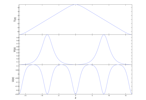
Figure 1: Plots of $T(z)$, $V(z)$ and $U(z)$ within a period of the tachyon field $[-2K(k)/\beta,2K(k)/\beta]$. Here $k=0.01$.

3.3 Numerical solution of eigenvalue equations

The periodicity of the solution and the potential for the fluctuations means that we need consider the range $0\leq z\leq K/\beta$, with eigenfunction taking either Dirichlet (D) or von Neumann (N) boundary conditions at each boundary. Hence there are four boundary conditions (BCs) which are listed and labelled in Table 1.

We solve the eigenvalue equations by numerical integration, “shooting” for the correct boundary condition at $z=K/\beta$, using the 4th/5th order Runge-Kutte integrator built into MATLAB, ode45. We adopted an absolute tolerance of $10^{-9}$ and a relative tolerance of $10^{-6}$ for all calculations in this paper.

BC(1): ND	BC(2): NN	BC(3): DD	BC(4): DN
$\phi^{\prime}(0)=0$	$\phi^{\prime}(0)=0$	$\phi(0)=0$	$\phi(0)=0$
$\phi(K/\beta)=0$	$\phi^{\prime}(K/\beta)=0$	$\phi(K/\beta)=0$	$\phi^{\prime}(K/\beta)=0$
$\phi(0)=1$	$\phi(0)=1$	$\phi^{\prime}(0)=1$	$\phi^{\prime}(0)=1$

Table 1: The four possible boundary conditions for the eigenfunctions of small fluctuations in the tachyon field about the static kink-antikink array. The letters D and N denote Dirichlet and von Neumann boundary conditions respectively. The last row gives the initial conditions for the numerical solution of the eigenvalue equation.

3.3.1 Fluctuation modes of low lying states

We first set $k=0.01$. In Figs 2, 3 and 4, normalized numerical solutions are presented in groups of four, whose eigenvalues are close together. We refer to them as zero mode states, first excited states and second excited states respectively. We denote normalised solutions by a tilde, and plot both $\tilde{\phi}(z)$ and $\delta\tilde{T}(z)$, which are defined as

$$\delta\tilde{T}(z)=\frac{\delta T(z)}{\int_{0}^{K/\beta}{|\delta T(z^{\prime})|^{2}dz^{\prime}}}$$ (3.19)

and

$$\tilde{\phi}(z)=\frac{\phi(z)}{\int_{0}^{K/\beta}{|\phi(z^{\prime})|^{2}dz^{\prime}}}.$$ (3.20)

Similarities and symmetries are clearer when looking at ${\phi}(z)$, as $\delta{T}(z)$ has a factor $V(z)/V_{0}$ which does not share the periodicity of the eigenfunctions, and suppresses the function away from the kinks. For example, eigenfunctions with BC(1) and BC(4) are related by the symmetry $z\to K/2\beta-z$, and therefore the eigenvalues are the same.

Because of the factor $V(z)/V_{m}$, the fluctuations away from the kinks are greatly suppressed when plotted in terms of $\delta T$, and the eigenfunctions look very similar near the (anti)kink at $z=K(k)/\beta$.

Fig. 1 contains the four states whose eigenvalues are very close to zero. Indeed, two with BC(1) and BC(4), and eigenvalues $\omega^{2}=-1.0672\times 10^{-8}$ and $\omega^{2}=-2.0095\times 10^{-9}$, are consistent with being numerical approximations to the true zero modes corresponding to the degeneracies in position $x_{0}$ (Fig. 1a) and amplitude $T_{0}$ (Fig. 1b) of the solution. Not only do they have very small eigenvalues, they also have the correct number and position of nodes.

We also have two low-lying modes with BC(2), one with a small negative eigenvalue, which we call $0^{-}$, and the other with a small positive one $0^{+}$. The negative eigenvalue reflects an instability in the system towards annihilation, where the kink-antikink pair moves together. There is no low-lying state with BC(3).

We can understand at least the ordering of the eigenvalues by studying the number of nodes of the eigenfunctions, using the standard result that more nodes means a higher eigenvalue.

We note first that the background has periodicity $4K(k)$, in which the eigenfunctions must also be periodic, and therefore have an even number of nodes. The lowest eigenvalue is associated with BC(2), which allows an eigenfunction with no nodes. BC(1,4) allow only 2 nodes, which are the zero modes. BC(2) also allows the 4-node eigenfunction shown in Fig. 2(d). BC(3) permits a minimum of 4 nodes which, because of its Dirichlet boundary conditions, are forced to be at the minimum of the potential $U(z)$, and it must therefore have a higher eigenvalue than the 4-node BC(2) eigenfunction, which peaks where the potential is lowest.

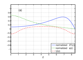
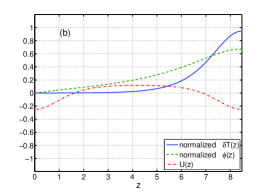
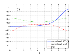
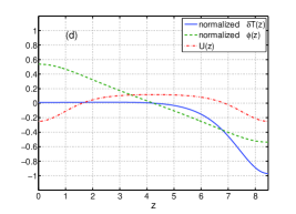
Figure 2: Normalized numerical solutions, $\delta\tilde{T}(z)$ and $\tilde{\phi}(z)$, of lowest eigenvalue modes with $k=0.01$, plotted with the potential $U(z)$ for comparison. (a) BC(1) and (b) BC(4) have eigenvalues which are consistent with zero, respectively $\omega^{2}=-1.0672\times 10^{-8}$ and $\omega^{2}=-2.0095\times 10^{-9}$. The other two figures are both under BC(2) and have two bound states with (c) $\omega^{2}=-0.0270$ (which we call $0^{-}$) and (d) $\omega^{2}=0.0433$ (which we call $0^{+}$). BC(3) (not shown in the figure) has no eigenvalues close to zero.

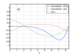
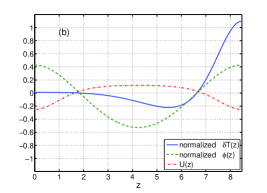
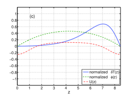
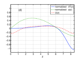
Figure 3: Normalized numerical solutions, $\delta\tilde{T}(z)$ and $\tilde{\phi}(z)$, of the first excited states with $k=0.01$ under the four boundary conditions: (a) BC(1), (b) BC(2), (c) BC(3) and (d) BC(4). Note that BC(1) and BC(4) have the same eigenvalue.

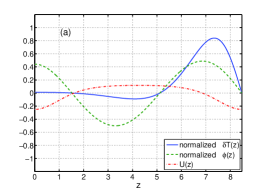
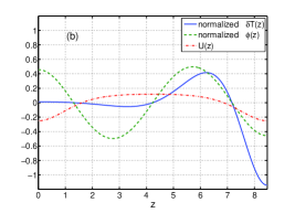
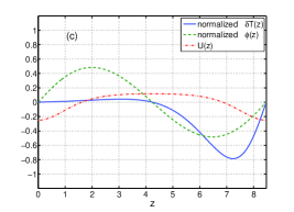
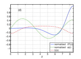
Figure 4: Normalized numerical solutions, $\delta\tilde{T}(z)$ and $\tilde{\phi}(z)$, of second excited states with $k=0.01$ under the four boundary conditions: (a) BC(1), (b) BC(2), (c) BC(3) and (d) BC(4). BC(1) and BC(4) have the same eigenvalue.

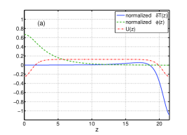
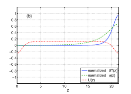
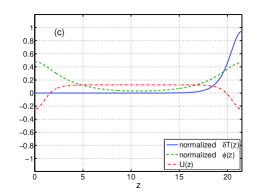
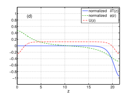
Figure 5: Normalized numerical solutions, $\delta\tilde{T}(z)$ and $\tilde{\phi}(z)$, of zero modes with $k=10^{-6}$. As for the case $k=10^{-2}$, (a) BC(1) and (b) BC(4) have eigenvalues very close to zero, which are respectively $\omega^{2}=-1.0765\times 10^{-8}$ and $\omega^{2}=1.6806\times 10^{-5}$. BC(2) also has two bound states with (c) $0^{-}$ mode: $\omega^{2}=-3.0842\times 10^{-4}$ and (d) $0^{+}$ mode: $\omega^{2}=3.6063\times 10^{-5}$. BC(3) has no zero eigenvalue.

3.3.2 Fluctuations with smaller $k$

Stable BPS daughter D$(p-1)$ branes form as $V_{0}$ approaches zero at the end of the tachyon condensation, so we should check the fluctuation behaviour as $k\rightarrow 0$. However, we were unable to get numerical solutions with very small $k$. In Fig. 5, we show the zero mode fluctuation with $k=10^{-6}$. Here it is even more obvious that fluctuations have support mostly near the brane position, both in $\phi$ and $\delta T$. The higher modes have similar properties. Therefore, we can expect that the fluctuations are confined to the branes more and more strongly when $k$ or $V_{0}$ tend to zero. We can interpret this as being consistent with the observation [27] in the homogeneous case that there are no propagating tachyon modes ($\omega^{2}\rightarrow 0$) in the vacuum when $V_{0}\rightarrow 0$.

3.3.3 Eigenvalues with varying $k$

We also investigate the eigenvalues against $\log k$ for all boundary conditions in Fig. 6, down to $\log k=-7$. We could not get eigenvalues for smaller $k$ for reasons of numerical precision.

As shown in Fig. 6a, eigenvalues $\omega^{2}$ seem to approach constant values with $k$ decreasing (which corresponds to letting $V_{0}$ tend to $0$ while keeping $V_{max}=1$ constant). We also see that the eigenvalues seem to assemble themselves into groups of four, which we referred to earlier as zero modes, first excited and second excited states. The grouping is not so clear for the second excited states, but supporting evidence is shown in Fig. 6b, where we see an approximate power law dependence for $\omega^{2}-\omega_{(n)\infty}^{2}$ against $k$, where $\omega_{(0)\infty}^{2}=0$ for the zero mode, $\omega_{(1)\infty}^{2}=0.135$ for the first excited state and $\omega_{(2)\infty}^{2}=0.169$ for the second one. Therefore, they should be the degenerate eigenvalues of all the four BCs in the limit of $T_{0}\rightarrow\infty$ or $k\rightarrow 0$.

The only bound states (whose eigenvalues are between 0 and $U_{max}\simeq 1/8$) are those associated with translations and changes in $V_{0}$, corroborating our analysis of the previous section with the approximate solution $T(z)\propto z$.

3.3.4 Eigenvalues at $k=0$ and correspondence with string ground states

The numerical results according for Fig. 5 imply a trend that, towards the end of the tachyon condensation, there are four degenerate zero modes under BC(1,2,4) (BC(2) contributes two). At the end of the decay, a stable solution consisting of an alternating series of D$p-1$ and anti-D$p-1$ branes form. It is interesting to compare the four zero modes of the tachyon field at $k=0$ to the bosonic massless states of the open string spectrum.

Without loss of generality, we assume that the $x$ direction is compactified on a circle with radius $R=1/\beta=\sqrt{2}$. The masses of open strings stretched between the parallel branes are

$$m^{2}=N+\left(\frac{\Delta{\theta}R}{2\pi}\right)^{2}-a,$$ (3.21)

where $N$ is the level number, $\triangle{\theta}$ is the angle difference between any two branes and we recall that $\alpha^{\prime}=1$. The parameter $a$ is the normal ordering constant which is $0$ for the Ramond (R) sector and $1/2$ for the Neveu-Schwarz (NS) sector. Between the two branes located on a circle, there are six ways to attach open strings: both ends on (i) D or (ii) $\overline{\textrm{D}}$ branes; stretching from D to $\overline{\textrm{D}}$ on both (iii) the right sides and (iv) the left sides of the branes; stretching from $\overline{\textrm{D}}$ to D on both (v) the right sides and (vi) the left sides. The bosonic massless states for the cases (i) and (ii) are the first excited states in the NS sector, which contain the transverse fluctuations of the brane. For (iii), (iv), (v) and (vi), the ground states are massless when $\Delta{\theta}=\pi$ and $R=\sqrt{2}$. These states become tachyonic if $R<\sqrt{2}$.

Hence we find a total of 6 bosonic massless states. Two are concerned with translations of the branes, two of them should be associated with brane-antibrane annihilation to D$p-3$ branes and the appearance of a new effective field theory [31], and the other two can be identified with the branes “melting” back into the unstable D$p$-brane. It is interesting that the original tachyon field, despite being singular, still contains sensible zero modes.

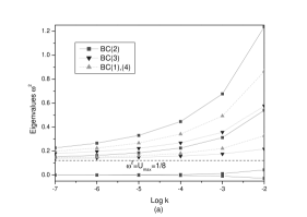
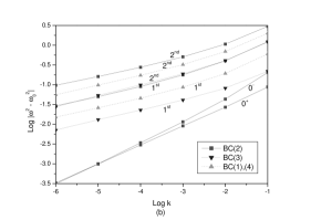
Figure 6: Eigenvalues of zero modes, first excited and second excited states against $\log k$ corresponding to the four BC respectively. Note that BC(1) and BC(4) have the same eigenvalues for all states because of symmetry.

4 Motion in moduli space

As we have seen, the condensation procession is essentially described by any one of the following parameters: $T_{0}$, $V_{0}=V(T_{0})$ and $k=V_{0}/V_{m}$. In the following, we study the time-dependent decay of the brane into a brane and an anti-brane by studying the motion of the $k$ modulus based on the solution of the static equation of motion.

We start from the $1+1$ dimensional effective action:

$$S=-\int dtdxV(T)\sqrt{1-\dot{T}^{2}-T^{\prime 2}}.$$ (4.22)

In the moduli space, we adopt the approximation $\dot{T}^{2}/(1+T^{\prime 2})\ll 1$, i.e., the tachyon evolves very slowly. Then an approximate action can be obtained, noting that $T^{\prime 2}=(V/V_{0})^{2}-1$:

$$S\simeq-\int dtdx\frac{V^{2}}{V_{0}}\left[1-\frac{1}{2}\left(\frac{V_{0}}{V}\right)^{2}\dot{T}^{2}\right].$$ (4.23)

When the second term is small enough, the Langrangian is exactly the energy of the static case in Eq. (2.5). We assume that there is a slow-motion solution with the approximate form of Eq. (2.4), with $k=V_{0}/V_{m}$ time-dependent. Hence

$$\dot{T}=-\frac{\tanh{(\beta T)}}{\beta k(1-k^{2})}\dot{k}.$$ (4.24)

Substituting into Eq. (4.23) and performing the integration over $x$, over a complete period of the tachyon field, we find

$$S=\int dtL(k,\dot{k})=-\frac{2\pi V_{m}}{\beta}\int dt\left[1-\frac{\dot{k}^{2}}{2\beta^{2}k(1+k)(1-k^{2})}\right].$$ (4.25)

where $L(k,\dot{k})$ is the Langrangian with parameters of $k$ and $\dot{k}$. The second term is a kinetic term, which can be expressed in terms of a variable $X(t)$ defined through:

$$\frac{1}{2}\dot{X}^{2}=\frac{1}{2}g(k)\dot{k}^{2},$$ (4.26)

where, $g(k)={1}/{[\beta^{2}k(1+k)(1-k^{2})]}$. The solution of $X$ is trivial: $X=X_{0}+vt$, where $X_{0}$ and $v$ are constants. Therefore from the relation between $k$ and $X$:

$$X=\int\sqrt{g(k)}dk=2\sqrt{\frac{\pi V_{m}}{\beta^{3}}}\tan^{-1}\sqrt{\frac{2k}{1-k}},$$ (4.27)

and we obtain the solution:

$$k(t)=\frac{4}{3+\cos{(c_{1}t+c_{0})}}-1,$$ (4.28)

where $c_{1}=v\sqrt{\beta^{3}/\pi V_{m}}$ and $c_{0}$ are constants. We discover that the D$p$ branes decay into D$p-1$ branes in a finite time $\triangle t=\sqrt{V_{m}\pi^{3}/\beta^{3}}/v$. This result is consistent with singularities appearing in finite time in time-dependent tachyon simulations [24, 23] and in boundary conformal field theory calculations [32]. We note that the solution is in fact periodic, and oscillates between the unstable D$p$ brane system and the daughter D$p-1$, $\overline{\textrm{D}}p-1$ brane system.

5 Conclusion

We have calculated numerically the low-lying modes of small fluctuations in the tachyon field around the static solution representing a periodic array of D$(p-1)$ and anti-D$(p-1)$ brane pairs. The potential for the fluctuations can be expressed in terms of Jacobi elliptic functions, and eigenvalue equations were solved numerically.

We find the two expected zero modes, corresponding to changes in the amplitude of the tachyon field between the kinks, and the position of the kinks. In addition there is a negative eigenvalue reflecting an attractive force between kinks and antikinks, which causes them to move together and annihilate.

There are higher excited states with eigenvalues $\omega^{2}>\beta^{2}/4$. In the language of the effective field theory these are unbound scattering states. In the limit that the tachyon field between the D$(p-1)$-branes tends to the vacuum, the eigenvalues of these states appear to tend to constant values (with $\omega^{2}$ still greater than $\beta^{2}/2$), and the support of the eigenfunctions shrinks with the width of the branes. Thus, although propagating modes are present, they disappear from the bulk between branes. This is consistent with the absence of propagating modes in the case of homogeneous tachyon condensation.

We have also attempted to make the possible link of the degenerate lowest tachyon fluctuation modes at the decay end $k=0$ to the open string spectra of ground states in the daughter brane, anti-brane system. With the daughter brane and anti-brane compactified on a circle along the $x$ direction, we found that the ground states of the open superstrings stretching between them are indeed massless. But there are 6 such states, which are two more than the zero modes we have obtained. The two extra zero massless states should correspond to standard brane-antibrane annihilation.

Finally, we note that there are approximate time-dependent solutions where the parameter of the solution Eq. (2.4), $V_{0}$ and $x_{0}$, become time-dependent. The time evolving solutions show that there are singularities appearing in a finite time, which is consistent with earlier work, but our solutions can be continued through the singularity to produce a periodic oscillation between a D$p$-brane and a D$p-1$-$\bar{\rm D}p-1$-brane pair.

- [1] M. R. Garousi, Tachyon couplings on non-bps d-branes and dirac-born-infeld action, Nucl. Phys. B584 (2000) 284–299, [hep-th/0003122].
- [2] E. A. Bergshoeff, M. de Roo, T. C. de Wit, E. Eyras, and S. Panda, T-duality and actions for non-bps d-branes, JHEP 05 (2000) 009, [hep-th/0003221].
- [3] A. Sen, Field theory of tachyon matter, Mod. Phys. Lett. A17 (2002) 1797–1804, [hep-th/0204143].
- [4] A. Mazumdar, S. Panda, and A. Perez-Lorenzana, Assisted inflation via tachyon condensation, Nucl. Phys. B614 (2001) 101–116, [hep-ph/0107058].
- [5] G. W. Gibbons, Cosmological evolution of the rolling tachyon, Phys. Lett. B537 (2002) 1–4, [hep-th/0204008].
- [6] M. Fairbairn and M. H. G. Tytgat, Inflation from a tachyon fluid?, Phys. Lett. B546 (2002) 1–7, [hep-th/0204070].
- [7] D. Choudhury, D. Ghoshal, D. P. Jatkar, and S. Panda, On the cosmological relevance of the tachyon, Phys. Lett. B544 (2002) 231–238, [hep-th/0204204].
- [8] L. Kofman and A. Linde, Problems with tachyon inflation, JHEP 07 (2002) 004, [hep-th/0205121].
- [9] M. Sami, P. Chingangbam, and T. Qureshi, Aspects of tachyonic inflation with exponential potential, Phys. Rev. D66 (2002) 043530, [hep-th/0205179].
- [10] G. Shiu and I. Wasserman, Cosmological constraints on tachyon matter, Phys. Lett. B541 (2002) 6–15, [hep-th/0205003].
- [11] P. Chingangbam, S. Panda, and A. Deshamukhya, Non-minimally coupled tachyonic inflation in warped string background, JHEP 02 (2005) 052, [hep-th/0411210].
- [12] A. Sen, So(32) spinors of type i and other solitons on brane- antibrane pair, JHEP 09 (1998) 023, [hep-th/9808141].
- [13] A. Sen, Bps d-branes on non-supersymmetric cycles, JHEP 12 (1998) 021, [hep-th/9812031].
- [14] D. Kutasov and V. Niarchos, Tachyon effective actions in open string theory, Nucl. Phys. B666 (2003) 56–70, [hep-th/0304045].
- [15] N. Lambert, H. Liu, and J. M. Maldacena, Closed strings from decaying d-branes, hep-th/0303139.
- [16] G. R. Dvali and S. H. H. Tye, Brane inflation, Phys. Lett. B450 (1999) 72–82, [hep-ph/9812483].
- [17] S. Sarangi and S. H. H. Tye, Cosmic string production towards the end of brane inflation, Phys. Lett. B536 (2002) 185–192, [hep-th/0204074].
- [18] D. Choudhury, D. Ghoshal, D. P. Jatkar, and S. Panda, Hybrid inflation and brane-antibrane system, JCAP 0307 (2003) 009, [hep-th/0305104].
- [19] K. Hashimoto and N. Sakai, Brane - antibrane as a defect of tachyon condensation, JHEP 12 (2002) 064, [hep-th/0209232].
- [20] G. Shiu, S. H. H. Tye, and I. Wasserman, Rolling tachyon in brane world cosmology from superstring field theory, Phys. Rev. D67 (2003) 083517, [hep-th/0207119].
- [21] J. M. Cline, H. Firouzjahi, and P. Martineau, Reheating from tachyon condensation, JHEP 11 (2002) 041, [hep-th/0207156].
- [22] A. Sen, Dirac-born-infeld action on the tachyon kink and vortex, Phys. Rev. D68 (2003) 066008, [hep-th/0303057].
- [23] N. Barnaby, A. Berndsen, J. M. Cline, and H. Stoica, Overproduction of cosmic superstrings, JHEP 06 (2005) 075, [hep-th/0412095].
- [24] J. M. Cline and H. Firouzjahi, Real-time d-brane condensation, Phys. Lett. B564 (2003) 255–260, [hep-th/0301101].
- [25] G. N. Felder, L. Kofman, and A. Starobinsky, Caustics in tachyon matter and other born-infeld scalars, JHEP 09 (2002) 026, [hep-th/0208019].
- [26] C.-j. Kim, Y.-b. Kim, and C. O. Lee, Tachyon kinks, JHEP 05 (2003) 020, [hep-th/0304180].
- [27] A. Sen, Tachyon dynamics in open string theory, Int. J. Mod. Phys. A20 (2005) 5513–5656, [hep-th/0410103].
- [28] P. Brax, J. Mourad, and D. A. Steer, Tachyon kinks on non bps d-branes, Phys. Lett. B575 (2003) 115–125, [hep-th/0304197].
- [29] L. D. Landau and E. M. Lifishitz, Quantum mechanics. Rergamon, Oxford, (1977).
- [30] I. S. Gradshteyn and I. M. Ryzhik, Table of Integrals, Series, and Products. Academic Press, (2000).
- [31] M. R. Garousi, D-brane anti-d-brane effective action and brane interaction in open string channel, JHEP 01 (2005) 029, [hep-th/0411222].
- [32] A. Sen, Time evolution in open string theory, JHEP 10 (2002) 003, [hep-th/0207105].