Symmetry breaking and quantum correlations in finite systems: Studies of quantum dots and ultracold Bose gases and related nuclear and chemical methods

Abstract

Investigations of emergent symmetry breaking phenomena occurring in small finite-size systems are reviewed, with a focus on the strongly correlated regime of electrons in two-dimensional semicoductor quantum dots and trapped ultracold bosonic atoms in harmonic traps. Throughout the review we emphasize universal aspects and similarities of symmetry breaking found in these systems, as well as in more traditional fields like nuclear physics and quantum chemistry, which are characterized by very different interparticle forces. A unified description of strongly correlated phenomena in finite systems of repelling particles (whether fermions or bosons) is presented through the development of a two-step method of symmetry breaking at the unrestricted Hartree-Fock level and of subsequent symmetry restoration via post Hartree-Fock projection techniques. Quantitative and qualitative aspects of the two-step method are treated and validated by exact diagonalization calculations.

Strongly-correlated phenomena emerging from symmetry breaking include:
(I) Chemical bonding, dissociation, and entanglement (at zero and finite magnetic fields) in quantum dot molecules and in pinned electron molecular dimers formed within a single anisotropic quantum dot, with potential technological applications to solid-state quantum-computing devices.
(II) Electron crystallization, with particle localization on the vertices of concentric polygonal rings, and formation of rotating electron molecules (REMs) in circular quantum dots. Such electron molecules exhibit ro-vibrational excitation spectra, in analogy with natural molecules.
(III) At high magnetic fields, the REMs are described by parameter-free analytic wave functions, which are an alternative to the Laughlin and composite-fermion approaches, offering a new point of view of the fractional quantum Hall regime in quantum dots (with possible implications for the thermodynamic limit).
(IV) Crystalline phases of strongly repelling bosons. In rotating traps and in analogy with the REMs, such repelling bosons form rotating boson molecules (RBMs). For a small number of bosons, the RBMs are energetically favored compared to the Gross-Pitaevskii solutions describing vortex formation.

We discuss the present status concerning experimental signatures of such strongly correlated states, in view of the promising outlook created by the latest experimental improvements that are achieving unprecedented control over the range and strength of interparticle interactions.

[Symmetry breaking and quantum correlations]

1 Introduction

1.1 Preamble

Fermionic or bosonic particles confined in manmade devices, i.e., electrons in two-dimensional (2D) quantum dots (QDs, referred to also as artificial atoms) or ultracold atoms in harmonic traps, can localize and form structures with molecular, or crystalline, characteristics. These molecular states of localized particles differ in an essential way from the electronic-shell-structure picture of delocalized electrons filling successive orbitals in a central-mean-field potential (the Aufbau principle), familiar from the many-body theory of natural atoms and the Mendeleev periodic table; they also present a different regime from that exhibited by a Bose-Einstein condensate (BEC, associated often with the mean-field Gross-Pitaevskii equation). The molecular states originate from strong correlations between the constituent repelling particles and they are called electron (and often Wigner) or boson molecules.

Such molecular states forming within a single confining potential well constitute new phases of matter and allow for investigations of novel strongly-correlated phenomena arising in physical systems with a range of materials’ characteristics unavailable experimentally (and theoretically unexplored) until recently. One example is the range of values of the socalled Wigner parameter (denoted as $R_{W}$ for charged particles and $R_{\delta}$ for neutral ones, see section 2.1.2) which expresses the relative strength of the two-body repulsion and the one-particle kinetic energy, reflecting and providing a measure of the strength of correlations in the system under study. For the two-dimensional systems which we discuss here, these values are often larger than the corresponding ones for natural atoms and molecules.

Other research opportunities offered by the quantum-dot systems are related to their relatively large (spatial) size (arising from a small electron effective mass and large dielectric constant), which allows the full range of orbital magnetic effects to be covered for magnetic fields that are readily attained in the laboratory (less than 40 T). In contrast, for natural atoms and molecules, magnetic fields of sufficient strength (i.e., larger than $10^{5}$ T) to produce novel phenomena related to orbital magnetism (beyond the perturbative regime) are known to occur only in astrophysical environments (e.g., on the surface of neutron stars) [1]. For ultracold gases, a similar extraordinary physical regime can be reached via the fast rotation of the harmonic trap.

In addition to the fundamental issues unveiled through investigations of molecular states in quantum dots, these strongly-correlated states are of technological significance because of the potential use of manmade nanoscale systems for the implementation of qubits and quantum logic gates in quantum computers.

The existence of electron and boson molecules is supported by large-scale exact diagonalization (EXD) calculations, which provide the ultimate theoretical test. The discovery of these “crystalline” states has raised important fundamental aspects, including the nature of quantum phase transitions and the conceptual issues relating to spontaneous symmetry breaking (SSB) in small finite-size systems.

The present report addresses primarily the physics, theoretical description, and fundamental many-body aspects of molecular (crystalline) states in small systems. For a comprehensive description of the electronic-shell-structure regime (Aufbau-principle regime) in quantum dots and of Bose-Einstein condensates in harmonic traps, see the earlier reviews by Kouwenhoven et al[2] (QDs), Reimann and Manninen [3] (QDs), Dalfovo et al[4] (BECs), and Leggett [5] (BECs). Furthermore, in larger quantum dots, the symmetries of the external confinement that lead to shell structure are broken, and such dots exhibit mesoscopic fluctuations and interplay between single-particle quantum chaos [6] and many-body correlations. For a comprehensive description of this mesoscopic regime in quantum dots, see the reviews by Beenakker [7] and Alhassid [8].

1.2 Spontaneous symmetry breaking: confined geometries versus extended systems

Spontaneous symmetry breaking is a ubiquitous phenomenon in the macroscopic world. Indeed, there is an abundance of macroscopic systems and objects that are observed, or can be experimentally prepared, with effective many-body ground states whose symmetry is lower than the symmetry of the underlying many-body quantum-mechanical Hamiltonian; one says that in such cases the system lowers its energy through spontaneous symmetry breaking, resulting in a state of lower symmetry and higher order. It is important to stress that macroscopic SSB strongly suppresses quantum fluctuations and thus it can be described appropriately by a set of non-linear mean-field equations for the “order parameter.” The appearance of the order parameter is governed by bifurcations associated with the non-linearity of the mean-field equations and has led to the notion of “emergent phenomena,” a notion that helped promote condensed-matter physics as a branch of physics on a par with high-energy particle physics (in reference to the fundamental nature of the pursuit in these fields; see the seminal paper by Anderson in Ref. [9]).

Our current understanding of the physics of SSB in the thermodynamic limit (when the number of particles $N\rightarrow\infty$) owes a great deal to the work of Anderson [10], who suggested that the broken-symmetry state can be safely taken as the effective ground state. In arriving at this conclusion Anderson invoked the concept of (generalized) rigidity. As a concrete example, one would expect a crystal to behave like a macroscopic body, whose Hamiltonian is that of a heavy rigid rotor with a low-energy excitation spectrum $L^{2}/2{\cal J}$ of angular-momentum $(L)$ eigenstates, with the moment of inertia ${\cal J}$ being of order $N$ (macroscopically large when $N\rightarrow\infty$). The low-energy excitation spectrum of this heavy rigid rotor above the ground-state ($L=0$) is essentially gapless (i.e., continuous). Thus although the formal ground state posseses continuous rotational symmetry (i.e., $L=0$), “there is a manifold of other states, degenerate in the $N\rightarrow\infty$ limit, which can be recombined to give a very stable wave packet with essentially the nature” of the broken-symmetry state (see p 44 in Ref. [10]).

As a consequence of the “macroscopic heaviness” as $N\rightarrow\infty$, the relaxation of the system from the wave packet state (i.e., the broken-symmetry state) to the exact symmetrical ground state becomes exceedingly long. Consequently, in this limit, when symmetry breaking occurs, there is practically no need to follow up with a symmetry restoration step; that is the symmetry-broken state is admissible as an effective ground state.

The present report addresses the much less explored question of symmetry breaking in finite condensed-matter systems with a small number of particles. For small systems, spontaneous symmetry breaking appears again at the level of mean-field description [e.g., the Hartree-Fock (HF) level]. A major difference from the $N\rightarrow\infty$ limit, however, arises from the fact that quantum fluctuations in small systems cannot be neglected. To account for the large fluctuations, one has to perform a subsequent post-Hartree-Fock step that restores the broken symmetries (and the linearity of the many-body Schrödinger equation). Subsequent to symmetry restoration, the ground state obeys all the original symmetries of the many-body Hamiltonian; however, effects of the mean-field symmetry breaking do survive in the properties of the ground state of small systems and lead to emergent phenomena associated with formation of novel states of matter and with characteristic behavior in the excitation spectra. In the following, we will present an overview of the current understanding of SSB in small systems focusing on the essential theoretical aspects, as well as on the contributions made by SSB-based approaches to the fast developing fields of two-dimensional semiconductor quantum dots and ultracold atomic gases in harmonic and toroidal traps.

1.3 Historical background from nuclear physics and chemistry

The mean field approach, in the form of the Hartree-Fock theory and of the Gross-Pitaevskii (GP) equation, has been a useful tool in elucidating the physics of finite-size fermionic and bosonic systems, respectively. Its applications cover a wide range of systems, from natural atoms, natural molecules, and atomic nuclei, to metallic nanoclusters, and most recently two-dimensional quantum dots and ultracold gases confined in harmonic (parabolic) traps. Of particular interest for the present review (due to spatial-symmetry-breaking aspects) has been the mean-field description of deformed nuclei [11, 12, 13] and metal clusters [14, 15, 16] (exhibiting ellipsoidal shapes). At a first level of description, deformation effects in these latter systems can be investigated via semi-empirical mean-field models, like the particle-rotor model [11] of Bohr and Mottelson (nuclei), the anisotropic-harmonic-oscillator model of Nilsson (nuclei [12] and metal clusters [14]), and the shell-correction method of Strutinsky (nuclei [17] and metal clusters [15, 16]). At the microscopic level, the mean field for fermions is often described [18, 19] via the self-consistent single-determinantal Hartree-Fock theory. At this level, the description of deformation effects mentioned above requires [18] consideration of unrestricted Hartree-Fock (UHF) wave functions that break explicitly the rotational symmetries of the original many-body Hamiltonian, but yield HF Slater determinants with lower energy compared to the symmetry-adapted restricted Hartree-Fock (RHF) solutions.

In earlier publications [20, 21, 22, 23, 24, 25, 26], we have shown that, in the strongly correlated regime, UHF solutions that violate the rotational (circular) symmetry arise most naturally in the case of two-dimensional single quantum dots, for both the cases of zero and high magnetic field; for a UHF calculation in the lowest Landau level (LLL), see also Ref. [27]. Unlike the case of atomic nuclei, however, where (due to the attractive interaction) symmetry breaking is associated primarily with quadrupole shape deformations (a type of Jahn-Teller distortion), spontaneous symmetry breaking in 2D quantum dots induces electron localization (or “crystallization”) associated with formation of electron, or Wigner, molecules). The latter name is used in honor of Eugene Wigner who predicted the formation of a classical rigid Wigner crystal for the 3D electron gas at very low densities [28]. We stress, however, that because of the finite size, Wigner molecules are most often expected to show a physical behavior quite different from the classical Wigner crystal. Indeed, for finite $N$, Wigner molecules exhibit analogies closer to natural molecules, and the Wigner-crystal limit is expected to be reached only for special limiting conditions.

For a small system the violation in the mean-field approximation of the symmetries of the original many-body Hamiltonian appears to be paradoxical at a first glance, and some times it has been described mistakenly as an “artifact” (in particular in the context of density-functional theory [29]). However, for the specific cases arising in Nuclear Physics and Quantum Chemistry, two theoretical developments had already resolved this paradox. They are: (1) the theory of restoration of broken symmetries via projection techniques [30, 31, 32], and (2) the group theoretical analysis of symmetry-broken HF orbitals and solutions in chemical reactions, initiated by Fukutome and coworkers [33] who used the symmetry groups associated with the natural 3D molecules. Despite the different fields, the general principles established in these earlier theoretical developments in nuclear physics and quantum chemistry have provided a wellspring of assistance in our investigations of symmetry breaking for electrons in quantum dots and bosons in harmonic traps. In particular, the restoration of broken symmetries in QDs and ultracold atomic traps via projection techniques constitutes a main theme of the present report.

The theory of restoration of broken symmetries has been developed into a sophisticated computational approach in modern nuclear physics. Using the broken-symmetry solutions of the Hartree-Fock-Bogoliubov theory (that accounts for nuclear pairing and superfluidity), this approach has been proven particularly efficient in describing the competition between shape deformation and pairing in nuclei. For some recent papers in nuclear physics, see, e.g., Refs. [34, 35, 36, 37, 38, 39]; for an application to superconducting metallic grains, see Ref. [40]. Pairing effects arise only in the case of attractive interactions and they are not considered in this report, since we deal only with repulsive two-body interactions.

1.4 Scope of the review

Having discussed earlier the general context and historical background from other fields regarding symmetry breaking, we give here an outline of the related methodologies and of the newly discovered strongly correlated phenomena that are discussed in this report in the area of condensed-matter nanosystems.

In particular, a two-step method [20, 21, 22, 23, 24, 25] of symmetry breaking at the unrestricted Hartree-Fock level and of subsequent post-Hartree-Fock restoration of the broken symmetries via projection techniques is reviewed for the case of two-dimensional (2D) semiconductor quantum dots and ultracold bosons in rotating traps with a small number ($N$) of particles. The general principles of the two-step method can be traced to nuclear theory (Peierls and Yoccoz, see the original Ref. [30], but also the recent Refs. [34, 35, 36, 37, 38, 39]) and quantum chemistry (Löwdin, see Ref. [31]); in the context of condensed-matter nanophysics and the physics of ultracold atomic gases, it constitutes a novel powerful many-body approach that has led to unexpected discoveries in the area of strongly correlated phenomena. The successes of the method have generated a promising theoretical outlook, bolstered by the unprecedented experimental and technological advances, pertaining particularly to control of system parameters (most importantly of the strength and variety of two-body interactions), that can be achieved in manmade nanostructures.

In conjunction with exact diagonalization calculations [26, 41, 42, 43, 44] and recent experiments [41, 44, 45], it is shown that the two-step method can describe a wealth of novel strongly correlated phenomena in quantum dots and ultracold atomic traps. These include:

(I) Chemical bonding, dissociation, and entanglement in quantum dot molecules [20, 22, 46] and in electron molecular dimers formed within a single elliptic QD [41, 42, 43, 44], with potential technological applications to solid-state quantum logic gates [47, 48, 49].

(II) Electron crystallization, with localization on the vertices of concentric polygonal rings, and formation of rotating electron molecules (REMs) in circular QDs. At zero magnetic field ($B$), the REMs can approach the limit of a rigid rotor [50, 51]; at high $B$, the REMs are highly floppy and “supersolid”-like, that is, they exhibit [51, 52, 53] a non-rigid rotational inertia [54], with the rings rotating independently of each other [52, 53].

(III) At high magnetic fields and under the restriction of the many-body Hilbert space to the lowest Landau level, the two-step method yields fully analytic many-body wave functions [24, 26], which are an alternative to the Jastrow/Laughlin (JL) [55] and composite-fermion (CF) [56, 57] approaches, offering a new point of view of the fractional quantum Hall regime (FQHE) [58, 59] in quantum dots (with possible implications for the thermodynamic limit).

Large scale exact-diagonalization calculations [26, 52, 53] support the results of the two-step method outlined in items II and III above.

(IV) The two-step method has been used [60] to discover crystalline phases of strongly repelling ultracold bosons (impenetrable bosons/ Tonks-Girardeau regime [61, 62]) in 2D harmonic traps. In the case of rotating traps, such repelling bosons form rotating boson molecules (RBMs) [63] that are energetically favorable compared to the Gross-Pitaevkii solutions, even for weak repulsion and, in particular, in the regime of GP vortex formation.

We will not discuss in this report specific applications of the two-step method to atomic nuclei. Rather, as the title conveys, the report aims at exploring the universal characteristics of quantum correlations arising from symmetry breaking across various fields dealing with small finite systems, such as 2D quantum dots, trapped ultracold atoms, and nuclei – and even natural 3D molecules. Such universal characteristics and similarities in related methodologies persist across the aforementioned fields in spite of the differences in the size of the physical systems and in the range, nature, and strength of the two-body interactions. For specific applications to atomic nuclei, the interested reader is invited to consult the nucler physics literature cited in this report.

Figure 1: (Color online) Synopsis of the method of hierarchical approximations (also referred to as the “two-step method,” emphasizing that symmetry breaking at the mean-field level must be accompanied by a subsequent post-Hartree-Fock step of symmetry restoration, with a subsequent further lowering of the energy). See text for a detailed description.

1.5 Using a hierarchy of approximations versus probing of exact solutions

Figure 1 presents a synopsis of the hierarchy of approximations associated with the two-step method, and in particular for the case of 2D quantum dots. (A similar synopsis can also be written for the case of bosonic systems.) This method produces approximate wave functions with lower energy at each approximation level (as indicated by the downward vertical arrow on the left of the figure).

At the lowest level of approximation (corresponding to higher energy with no correlations included), one places the restricted Hartree-Fock, whose main restriction is the double occupancy (up and down spins) of each space orbital. The many-body wave function is a single Slater determinant associated with a “central mean field.” The RHF preserves all spin and space symmetries. For 2D quantum dots, the single-particle density [also referred to as electron density ($e$-density)] is circularly symmetric.

The next approximation involves the unrestricted Hartree-Fock, which employs different space orbitals for the two different spin directions. The UHF preserves the spin projection, but allows the total-spin and space symmetries (i.e., rotational symmetries or parity) to be broken. The broken symmetry solutions, however, are not devoid of any symmetry; they exhibit characteristic lower symmetries (point-group symmetries) that are explicit in the electron densities. The UHF many-body wave function is a single Slater determinant associated with a “non-central mean field.”

Subsequent approximations aim at restoring the broken symmetries via projection techniques. The restoration-of-symmetry step goes beyond the mean field approximation and it provides a many-body wave function $|\Phi^{\rm PRJ}\rangle$ that is a linear superposition of Slater determinants (see detailed description in section 2.2 below). The projected (PRJ) many-body wave function $|\Phi^{\rm PRJ}\rangle$ preserves all the symmetries of the original many-body Hamiltonian; it has good total spin and angular momentum quantum numbers, and as a result the circular symmetry of the electron densities is restored.

However, the lower (point-group) spatial symmetry found at the broken-symmetry UHF level (corresponding to the first step in this method) does not disappear. Instead, it becomes intrinsic or hidden, and it can be revealed via an inspection of conditional probability distributions (CPDs), defined as (within a proportionality constant)

$$P({\bf r},{\bf r}_{0})=\langle\Phi^{\rm PRJ}|\sum_{i\neq j}\delta({\bf r}_{i}-{\bf r})\delta({\bf r}_{j}-{\bf r}_{0})|\Phi^{\rm PRJ}\rangle,$$ (1.1)

where $\Phi^{\rm PRJ}({\bf r}_{1},{\bf r}_{2},\ldots,{\bf r}_{N})$ denotes the projected many-body wave function under consideration.

If one needs to probe the intrinsic spin distribution of the localized electrons, one has to consider spin-resolved two-point correlation functions (spin-resolved CPDs), defined as

$$P_{\sigma\sigma_{0}}({\bf r},{\bf r}_{0})=\langle\Phi^{\rm{PRJ}}|\sum_{i\neq j}\delta({\bf r}-{\bf r}_{i})\delta({\bf r}_{0}-{\bf r}_{j})\delta_{\sigma\sigma_{i}}\delta_{\sigma_{0}\sigma_{j}}|\Phi^{\rm{PRJ}}\rangle.$$ (1.2)

The spin-resolved CPD gives the spatial probability distribution of finding a second electron with spin projection $\sigma$ under the condition that a first electron is located (fixed) at ${\bf r}_{0}$ with spin projection $\sigma_{0}$; $\sigma$ and $\sigma_{0}$ can be either up $(\uparrow$) or down ($\downarrow$). The meaning of the space-only CPD in (1.1) is analogous, but without consideration of spin.

Further signatures of the intrinsic lower symmetry occur in the excitation spectra of circular quantum dots that exhibit ro-vibrational character related to the intrinsic molecular structure, or in the dissociation of quantum dot molecules.

As the scheme in figure 1 indicates, the mean-field HF equations are non-linear and the symmetry breaking is associated with the appearance of bifurcations in the total HF energies. The occurrence of such bifurcations cannot be predicted a priori from a mere inspection of the many-body Hamiltonian itself; it is a genuine many-body effect that belongs to the class of so-called emergent phenomena [9, 64, 65] that may be revealed only through the solutions of the Hamiltonian themselves (if obtainable) or through experimental signatures. We note that the step of symmetry restoration recovers also the linear properties of the many-body Schrödinger equation.

The relation between quantum correlations and the two-step method (also called the method of hierarchical approximations) is portrayed by the downward vertical arrow on the right of figure 1. Indeed, the correlation energy is defined [66] as the difference between the restricted Hartree-Fock and exact ground-state energies, i.e.,

$$E_{\rm corr}=E_{\rm RHF}-E_{\rm EXD}.$$ (1.3)

As seen from figure 1, starting with the broken-symmetry UHF solution, each further approximation captures successively a larger fraction of the correlation energy (1.3); a specific example of this process is given in figure 5 below (in section 2.2).

An alternative approach for studying the emergence of crystalline structures is the exact-diagonalizaion method that will be discussed in detail in section 4.1. Like the projected wave functions, the EXD many-body wave functions preserve of course all the symmetries of the original Hamiltonian. As a result, the intrinsic, or hidden, point-group symmetry associated with particle localization and molecule formation is not explicit, but it is revealed through inspection of CPDs [one simply uses the exact-diagonalization wave function $\Phi^{\rm EXD}({\bf r}_{1},{\bf r}_{2},\ldots,{\bf r}_{N})$ in Equation (1.1)] and Equation (1.2), or recognized via characteristic trends in the calculated excitation spectra. When feasible, the EXD results provide a definitive answer in terms of numerical accuracy, and as such they serve as a test to the results obtained through approximation methods (e.g., the above two-step method). However, the underlying physics of electron or boson molecule formation is less transparent when analyzed with the exact-diagonalization method compared to the two-step approach. Indeed, many exact-diagonalization studies of 2D quantum dots and trapped bosons in harmonic traps have focused simply on providing high accuracy energetics and they omitted calculation of CPDs. However, the importance of using CPDs as a tool for probing the many-body wave functions cannot be overstated. For example, while exact-diagonalization calculations for bosons in the lowest Landau level have been reported rather early [67, 68, 69, 70, 71], the analysis in these studies did not include calculations of the CPDs, and consequently formation of rotating boson molecules and particle “crystallization” was not recognized (for further discussion of these issues, see Romanovsky et al[60, 63] and Baksmaty et al[72]).

From the above, it is apparent that both methods, i.e., the two-step method and the exact-diagonalization one, complement each other, and it is in this spirit that we use them in this report.

1.6 Experimental signatures of quantum correlations

Historically, the isolation of a small number ($N<20$) of electrons down to a single electron was experimentally realized in the so-called “vertical” quantum dots [2]. The name vertical QDs derives from the fact that the leads and voltage gates are located in a vertical arrangement, on top and below the two-dimensional dot. At zero magnetic field, experimental measurements [2, 73] of addition energies,

$$\Delta^{2}E_{N}=\mu_{N+1}-\mu_{N},$$ (1.4)

where the chemical potential $\mu_{N}=E_{N}-E_{N-1}$, indicated that correlation effects at zero and low $B$ are rather weak in such dots, a property that later was attributed to the strong screening of the Coulomb interaction in these devices. The measured addition energies exhibited maxima at closed electronic shells ($N=2,6,12,\ldots$) and at mid-shells ($N=4,9,\ldots$) in agreement with a 2D-harmonic-oscillator central-mean-field model and the Hund’s rules, and in analogy with the Aufbau principle and the physics of natural 3D atoms. It was found that the measured ground-state energy spectra for low magnetic fields could be understood on the basis of a simple “constant-interaction” model where the effect of the two-body Coulomb interaction is reduced phenomenologically to an overall classical capacitance, $C$, characterizing the charging energy $Z^{2}e^{2}/(2C)$ of the quantum dot.

As a result of screening, strong correlation effects and formation of Wigner molecules can be expected to occur in vertical dots particularly under the influence of high magnetic fields. Evidence about the formation of Wigner molecules in vertical quantum dots has been provided recently in Ref. [74], where measured ground-state spectra as a function of $B$ for $N=3e$ and $N=4e$ were reanalyzed with exact-diagonalization calculations that included screening. At the time of submission of this report, a second ground-state crossing at high $B$ due to strong correlations was also demonstrated experimentally in a two-electron vertical quantum dot with an external confinement that was smaller than the previously used ones [75].

Early theoretical work [20] at zero magnetic field using simply the symmetry broken UHF solutions suggested that an unscreened Coulomb repulsion may result in a violation of Hund’s rules. However, following the two-step method of Refs. [20, 21, 22, 23, 24, 25], it has been shown [76] most recently that the companion step of symmetry restoration recovers the Hund’s rules in the case of $N=4e$.

In addition, the $B=0$ results of Ref. [20] suggested that both the maxima of the addition energies at closed shells and at mid-shells become gradually weaker (and they eventually disappear) as the strength of the Coulomb interaction (and consequently the strength of correlations) increases, leading to formation of “strong” Wigner molecules. The qualitative trend of formation of strong Wigner molecules obtained from a relatively simple UHF calculation at $B=0$ has been confirmed later by more accurate EXD [50, 77] and quantum Monte Carlo [78] calculations, as well as through symmetry restoration calculations [23, 76], although its experimental demonstration remains still a challenge.

A more favorable experimental configuration for the development and observation of strong interelectron correlations is the so-called “lateral” dot, where the leads and gates are located on the sides of the dot and thus screening effects are reduced. Tunability of these dots down to a single electron has been achieved only in the last few years [79]. Most recently, continually improving experimental techniques have allowed precise measurements of excitation spectra of $2e$ lateral (and anisotropic) quantum dots at zero and low magnetic fields [41, 45, 80]. As discussed in detail in section 5, the behavior of these excitation spectra [41, 45] as a function of $B$ provides unambiguous signatures for the presence of strong correlations and the formation of Wigner molecules.

Experimentally observed behavior of two electrons in lateral double QDs [81] provides further evidence for strong correlation phenomena. Indeed, instead of successively populating delocalized states over both QDs according to a molecular-orbital scheme, the two electrons localize on the individual dots according to a Heitler-London picture [82]. Theoretically, such strongly correlated phenomena in double quantum dots were described in Refs. [20, 22, 46]; see section 2.1.4 below.

Correlations are expected to influence not only the spectral properties of quantum dots, but also to effect transport characteristics. Indeed correlation effects may underlie the behavior of the transmission amplitudes (magnitude and phase) of an electron tunneling through a quantum dot. Such transmission measurements have been performed using Aharonov-Bohm interferometry [83], and an interpretation involving strongly correlated states in the form of Wigner molecules has been proposed recently [84]. The quantity that links transport experiments with many-body theory of electrons in QDs is the overlap between many-body states with $N-1$ and $N$ electrons, i.e., $\langle\Phi(N-1)|c_{j}|\Phi(N)\rangle$, where $c_{j}$ annihilates the $j$th electron.

The strength of correlations in quantum dots at zero $B$ can be quantified by the Wigner parameter $R_{W}$, which is the ratio between the strength of the Coulomb repulsion and the one-electron kinetic energy (see section 2.1.2). Naturally, for the case of neutral repelling bosons, the corresponding parameter is the ratio between the strength of the contact interaction and the one-particle kinetic energy in the harmonic trap, and it is denoted as $R_{\delta}$. Larger values of these parameters ($R_{W}$ or $R_{\delta}$) result in stronger correlation effects.

Progress in the ability to experimentally control the above parameters has been particularly impressive in the case of ultracold trapped bosons. Indeed, realizations of continuous tunability of $R_{\delta}$ over two orders of magnitude (from 1 to 5 [85] and from 5 to 200 [86]) has been most recently reported in quasi-linear harmonic traps. Such high values of $R_{\delta}$ allowed experimental realization of novel strongly correlated states drastically different from a Bose-Einstein condensate. This range of high values of $R_{\delta}$ is known as the Tonks-Girardeau regime and the corresponding states are one-dimensional analogues of molecular structures made out of localized bosons. In two dimenional traps, it has been predicted that such large values of $R_{\delta}$ lead to the emergence of crystalline phases [60, 63].

The high experimental control of optical lattices has also been exploited for the creation [87] of novel phases of ultracold bosons analogous to Mott insulators; such phases are related to the formation of electron puddles discussed in section 2.1.4 and to the fragmentation of Bose-Einstein condensates [88].

1.7 Plan of the report

The plan of the report can be visualized through the table of contents. Special attention has been given to the Introduction, which offers a general presentation of the subject of symmetry breaking and quantum correlations in confined geometries – including a discussion of the differences with the case of extended systems, a historical background from other fields, and a diagrammatic synopsis of the two-step method of symmetry breaking/symmetry restoration.

The theoretical framework and other technical methodological background are presented in Section 2 (symmetry breaking/symmetry restoration in quantum dots), Section 3 (symmetry breaking/symmetry restoration for trapped ultracold bosons), and Section 4 (exact-diagonalization approaches). Section 4 includes also a commentary on quantum Monte Carlo methods.

For the case of semiconductor quantum dots, the main results and description of the strongly correlated regime are presented in Sections 5, 6, and 7, with Section 5 focusing on the case of two electrons and its historical significance. Section 8 is devoted to a description of the strongly-correlated regime of trapped repelling bosons.

Finally, a summary is given in Section 9, and the Appendix offers an outline of the Darwin-Fock single-particle spectra for a two-dimensional isotropic oscillator under a perpendicular magnetic field or under rotation.

We note that the sections on trapped bosons (Section 3 and Section 8) can be read independently from the sections on quantum dots.

2 Symmetry breaking and subsequent symmetry restoration for electrons in confined geometries: Theoretical framework

The many-body Hamiltonian describing $N$ electrons confined in a two-dimensional QD and interacting via a Coulomb repulsion is written as

$${\cal H}=\sum_{i=1}^{N}H(i)+\sum_{i=1}^{N}\sum_{j>i}^{N}\frac{e^{2}}{\kappa r_{ij}}.$$ (2.1)

In Equation (2.1), $\kappa$ is the dielectric constant of the semiconducting material and $r_{ij}=|{\bf r}_{i}-{\bf r}_{j}|$. The single-particle Hamiltonian in a perpendicular external magnetic field $B$ is given by

$$H=\frac{({\bf p}-e{\bf A}/c)^{2}}{2m^{*}}+V(x,y)+\frac{g^{*}\mu_{B}}{\hbar}{\bf B\cdot s},$$ (2.2)

where the external confinement is denoted by $V(x,y)$, the vector potential ${\bf A}$ is given in the symmetric gauge by

$${\bf A}({\bf r})=\frac{1}{2}{\bf B}\times{\bf r}=\frac{1}{2}(-By,Bx,0),$$ (2.3)

and the last term in (2.2) is the Zeeman interaction with $g^{*}$ being the effective Landé factor, $\mu_{B}$ the Bohr magneton, ${\bf s}$ the spin of an individual electron and $m^{*}$ is the effective electron mass. The external potential confinement $V(x,y)$ can assume various parametrizations in order to model a single circular or elliptic quantum dot, or a quantum dot molecule. Of course, in the case of an elliptic QD, one has

$$V(x,y)=\frac{1}{2}m^{*}(\omega_{x}^{2}x^{2}+\omega_{y}^{2}y^{2}),$$ (2.4)

which reduces to the circular QD potential when $\omega_{x}=\omega_{y}=\omega_{0}$. The appropriate parametrization of $V(x,y)$ in the case of a double QD is more complicated. In our work, we use a parametrization based on a 2D two-center oscillator with a smooth necking. This latter parametrization is described in detail in Refs. [23, 46], where readers are directed for further details. In contrast with other parametrizations based on two displaced inverted Gaussians [89], the advantage of the two-center oscillator is that the height of the interdot barrier, the distance between the dots, the ellipticity of each dot, and the gate potentials of the two dots (i.e., the relative potential wells in the neighboring dots) can be varied independently of each other.

A prefactor multiplying the Coulomb term in Equation (2.1) (being either an overall constant $\gamma$ as in section 5.1 below, or having an appropriate position-dependent functional form [42, 43]) is used to account for the reduction of the Coulomb interaction due to the finite thickness of the electron layer and to additional screening (beyond that produced by the dielectric constant of the material) arising from the formation of image charges in the gate electrodes [90].

2.1 Mean-field description and unrestricted Hartree-Fock

Vast literature is available concerning mean-field studies of electrons in quantum dots. Such publications are divided mainly into applications of density functional theory [3, 91, 92, 93, 94, 95, 96] and the use of Hartree-Fock methods [20, 25, 27, 93, 97, 98, 99, 100, 101, 102, 103, 104]. The latter include treatments according to the restricted Hartree-Fock [97], unrestricted Hartree-Fock with spin, but not space, symmetry breaking [98, 99, 100], unrestricted Hartree-Fock with spin and/or space symmetry breaking [20, 25, 27, 93, 101, 102, 103], and the so-called Brueckner Hartree-Fock [104, 105].

From the several Hartree-Fock variants mentioned above, only the UHF with consideration of both spin and space symmetry unrestrictions has been able to describe formation of Wigner molecules, and in the following we will exclusively use this unrestricted version of Hartree-Fock theory. The inadequacy of the density-functional theory in describing Wigner molecules will be discussed in section 2.3.

2.1.1 The self-consistent Pople-Nesbet equations.

The unrestricted Hartree-Fock equations used by us are an adaptation of the Pople-Nesbet [106] equations described in detail in Ch 3.8 of Ref. [19]. For completeness, we present here a brief description of these equations, along with pertinent details of their computational implementation by us to the 2D case of semiconductor QDs.

We start by requesting that the unrestricted Hartree-Fock many-body wave function for $N$ electrons is represented by a single Slater determinant

$$\Psi_{\rm UHF}({\bf x}_{1},\ldots,{\bf x}_{N})=\frac{1}{\sqrt{N!}}{\rm det}[\chi_{1}({\bf x}_{1}),\chi_{2}({\bf x}_{2}),\ldots,\chi_{N}({\bf x}_{N}],$$ (2.5)

where $[\chi_{i}({\bf x})]$ are a set of $N$ spin orbitals, with the index ${\bf x}$ denoting both the space and spin coordinates. Furthermore, we take $\chi_{i}({\bf x})=\psi_{i}({\bf r})\alpha$ for a spin-up electron and $\chi_{i}({\bf x})=\psi_{i}({\bf r})\beta$ for a spin-down electron. As a result, the UHF determinants in this report are eigenstates of the projection of the total spin with eigenvalue $S_{z}=(N^{\alpha}-N^{\beta})/2$, where $N^{\alpha(\beta)}$ denotes the number of spin up (down) electrons. However, these Slater determinants are not eigenstates of the square of the total spin, ${\bf S}^{2}$, except in the fully spin polarized case.

According to the variational principle, the best spin orbitals must minimize the total energy $\langle\Psi_{\rm UHF}|{\cal H}|\Psi_{\rm UHF}\rangle$. By varying the spin orbitals $[\chi_{i}({\bf x})]$ under the constraint that they remain orthonormal, one can derive the UHF Pople-Nesbet equations described below.

A key point is that electrons with $\alpha$ (up) spin will be described by one set of spatial orbitals $\{\psi^{\alpha}_{j}|j=1,2,\dots,K\}$, while electrons with $\beta$ (down) spin are described by a different set of spatial orbitals $\{\psi^{\beta}_{j}|j=1,2,\ldots,K\}$; of course in the restricted Hartree-Fock $\psi^{\alpha}_{j}=\psi^{\beta}_{j}=\psi_{j}$. Next, one introduces a set of basis functions $\{\varphi_{\mu}|\mu=1,2,\ldots,K\}$ (constructed to be orthonormal in our 2D case), and expands the UHF orbitals as

$$\psi^{\alpha}_{i}=\sum_{\mu=1}^{K}C_{\mu i}^{\alpha}\varphi_{\mu},~{}~{}~{}i=1,2,\ldots,K,$$ (2.6)

$$\psi^{\beta}_{i}=\sum_{\mu=1}^{K}C_{\mu i}^{\beta}\varphi_{\mu},~{}~{}~{}i=1,2,\ldots,K.$$ (2.7)

The UHF equations are a system of two coupled matrix eigenvalue problems resolved according to up and down spins,

$${\bf F}^{\alpha\beta}{\bf C}^{\alpha}={\bf C}^{\alpha}{\bf E}^{\alpha}$$ (2.8)

$${\bf F}^{\beta\alpha}{\bf C}^{\beta}={\bf C}^{\beta}{\bf E}^{\beta},$$ (2.9)

where ${\bf F}^{\alpha\beta(\beta\alpha)}$ are the Fock-operator matrices and ${\bf C}^{\alpha(\beta)}$ are the vectors formed with the coefficients in the expansions (2.6) and (2.7). The matrices ${\bf E}^{\alpha(\beta)}$ are diagonal, and as a result equations (2.8) and (2.9) are canonical (standard). Notice that noncanonical forms of HF equations are also possible (see Ch 3.2.2 of Ref. [19]). Since the self-consistent iterative solution of the HF equations can be computationally implemented only in their canonical form, canonical orbitals and solutions will always be implied, unless otherwise noted explicitly. We note that the coupling between the two UHF equations (2.8) and (2.9) is given explicitly in the expressions for the elements of the Fock matrices below [(2.12) and (2.13)].

Introducing the density matrices ${\bf P}^{\alpha(\beta)}$ for $\alpha(\beta)$ electrons,

$$P^{\alpha}_{\mu\nu}=\sum_{a}^{N^{\alpha}}C^{\alpha}_{\mu a}(C^{\alpha}_{\nu a})^{*}$$ (2.10)

$$P^{\beta}_{\mu\nu}=\sum_{a}^{N^{\beta}}C^{\beta}_{\mu a}(C^{\beta}_{\nu a})^{*},$$ (2.11)

where $N^{\alpha}+N^{\beta}=N$, the elements of the Fock-operator matrices are given by

$$F^{\alpha\beta}_{\mu\nu}=H_{\mu\nu}+\sum_{\lambda}\sum_{\sigma}P^{\alpha}_{\lambda\sigma}[(\mu\sigma|\nu\lambda)-(\mu\sigma|\lambda\nu)]+\sum_{\lambda}\sum_{\sigma}P^{\beta}_{\lambda\sigma}(\mu\sigma|\nu\lambda)$$ (2.12)

$$F^{\beta\alpha}_{\mu\nu}=H_{\mu\nu}+\sum_{\lambda}\sum_{\sigma}P^{\beta}_{\lambda\sigma}[(\mu\sigma|\nu\lambda)-(\mu\sigma|\lambda\nu)]+\sum_{\lambda}\sum_{\sigma}P^{\alpha}_{\lambda\sigma}(\mu\sigma|\nu\lambda),$$ (2.13)

where $H_{\mu\nu}$ are the elements of the single electron Hamiltonian (with an external magnetic field $B$ and an appropriate potential confinement), and the Coulomb repulsion is expressed via the two-electron integrals

$$(\mu\sigma|\nu\lambda)=\frac{e^{2}}{\kappa}\int\rmd{\bf r}_{1}\rmd{\bf r}_{2}\varphi^{*}_{\mu}({\bf r}_{1})\varphi^{*}_{\sigma}({\bf r}_{2})\frac{1}{|{\bf r}_{1}-{\bf r}_{2}|}\varphi_{\nu}({\bf r}_{1})\varphi_{\lambda}({\bf r}_{2}),$$ (2.14)

with $\kappa$ being the dielectric constant of the semiconductor material. Of course, the Greek indices $\mu$, $\nu$, $\lambda$, and $\sigma$ run from 1 to $K$.

The system of the two coupled UHF matrix equations (2.8) and (2.9) is solved selfconsistently through iteration cycles. For obtaining the numerical solutions, we have used a set of $K$ basis states $\varphi_{i}$’s that are chosen to be the product wave functions formed from the eigenstates of one-center (single QD) and/or two-center [22, 46] (double QD) one-dimensional oscillators along the $x$ and $y$ axes. Note that for a circular QD a value $K=78$ corresponds to all the states of the associated 2D harmonic oscillator up to and including the 12th major shell.

The UHF equations preserve at each iteration step the symmetries of the many-body Hamiltonian, if these symmetries happen to be present in the input (initial) electron density of the iteration (see section 5.5 of Ref. [18]). The input densities into the iteration cycle are controlled by the values of the $P^{\alpha}_{\lambda\sigma}$ and $P^{\beta}_{\lambda\sigma}$ matrix elements. Two cases arise in practice: (i) Symmetry adapted RHF solutions are extracted from (2.8) and (2.9) by using as input $P^{\alpha}_{\lambda\sigma}=P^{\beta}_{\lambda\sigma}$=0 for the case of closed shells (with or without an infinitesimally small $B$ value). For open shells, one needs to use an infinitesimally small value of $B$. With these choices, the output of the first iteration (for either closed or open shells) is the single-particle spectrum and corresponding electron densities at $B=0$ associated with the Hamiltonian in (2.2) (the small value of $B$ mentioned above guarantees that the single-particle total and orbital densities are circular). (ii) For obtaining broken-symmetry UHF solutions, the input densities must be different in an essential way from the ones mentioned above. We have found that the choice $P^{\alpha}_{\lambda\sigma}=1$ and $P^{\beta}_{\lambda\sigma}=0$ usually produces broken-symmetry solutions (in the regime where symmetry breaking occurs).

Having obtained the selfconsistent solution, the total UHF energy is calculated as

$$E_{\rm UHF}=\frac{1}{2}\sum_{\mu}\sum_{\nu}[(P^{\alpha}_{\nu\mu}+P^{\beta}_{\nu\mu})H_{\mu\nu}+P^{\alpha}_{\nu\mu}F^{\alpha\beta}_{\mu\nu}+P^{\beta}_{\nu\mu}F^{\beta\alpha}_{\mu\nu}].$$ (2.15)

We note that the Pople-Nesbet UHF equations are primarily employed in Quantum Chemistry for studying the ground states of open-shell molecules and atoms. Unlike our studies of QDs, however, such chemical UHF studies consider mainly the breaking of the total spin symmetry, and not that of the space symmetries. As a result, for purposes of emphasis and clarity, we have often used (see, e.g., our previous papers) prefixes to indicate the specific unrestrictions (that is removal of symmetry restrictions) involved in our UHF solutions, i.e., the prefix s- for the total-spin and the prefix S- for the space unrestriction.

The emergence of broken-symmetry solutions is associated with instabilities of the restricted HF solutions, i.e., the restricted HF energy is an extremum whose nature as a minimum or maximum depends on the positive or negative value of the second derivative of the HF energy. The importance of this instability problem was first highlighted in a paper by Overhauser [107]. Soon afterwards, the general conditions for the appearance of such instabilities (analyzed within linear response and the random-phase approximation) were discussed by Thouless in the context of nuclear physics [108]. Subsequently, the Hartree-Fock stability/instability conditions were re-examined [109, 110], using a language from (and applications to) the field of quantum chemistry. For comprehensive reviews of mean-field symmetry breaking and the Hartree-Fock methods and instabilities in the context of quantum chemistry, see the collection of papers in Ref. [111].

2.1.2 The Wigner parameter and classes of spontaneous symmetry breaking solutions.

Using the self-consistent (spin-and-space) unrestricted Hartree-Fock equations presented in the previous section, we found [20], for zero and low magnetic fields, three classes of spontaneous symmetry breakings in circular single QDs and in lateral quantum dot molecules (i.e., formation of ground states of lower symmetry than that of the confining potentials). These include the following:

(I) Wigner molecules in both QDs and quantum dot molecules, i.e., (spatial) localization of individual electrons within a single QD or within each QD comprising the quantum dot molecule.

(II) formation of electron puddles in quantum dot molecules, that is, localization of the electrons on each of the individual dots comprising the quantum dot molecule, but without localization within each dot, and

(III) pure spin-density waves (SDWs) which are not accompanied by spatial localization of the electrons [91].

Figure 2: (Color online) UHF electron density in a parabolic QD for $N=19$ and $S_{z}=19/2$, exhibiting breaking of the circular symmetry at $R_{W}=5$ and $B=0$. The choice of the remaining parameters is: $\hbar\omega_{0}=5$ meV and $m^{*}=0.067m_{e}$. Distances are in nanometers and the electron density in $10^{-4}$ nm^-2.

It can be shown that a central-mean-field description (associated with the RHF) at zero and low magnetic fields may apply in the case of a circular QD only for low values of the Wigner parameter

$$R_{\rm W}\equiv Q/\hbar\omega_{0},$$ (2.16)

where $Q$ is the Coulomb interaction strength and $\hbar\omega_{0}$ is the energy quantum of the harmonic potential confinement (being proportional to the one-particle kinetic energy); $Q=e^{2}/(\kappa l_{0})$, with $\kappa$ being the dielectric constant, $l_{0}=(\hbar/(m^{*}\omega_{0}))^{1/2}$ the spatial extension of the lowest state’s wave function in the harmonic (parabolic) confinement, and $m^{*}$ the effective electron mass.

Furthermore, we find that Wigner molecules (SSB class I) occur in both QDs and quantum dot molecules for $R_{\rm W}>1$. Depending on the value of $R_{W}$, one may distinguish between “weak” (for smaller $R_{W}$ values) and “strong” (for larger $R_{W}$ values) Wigner molecules, with the latter termed sometimes as “Wigner crystallites” or “electron crystallites.” The appearance of such crystalline structures may be regarded as a quantum phase transition of the electron liquid upon increase of the parameter $R_{W}$. Of course, due to the finite size of QDs, this phase transition is not abrupt, but it develops gradually as the parameter $R_{W}$ varies.

For quantum dot molecules with $R_{\rm W}<1$, Wigner molecules do not develop and instead electron puddles may form (SSB class II). For single QDs with $R_{\rm W}<1$, we find in the majority of cases that the ground-states exhibit a central-mean-field behavior without symmetry breaking; however, at several instances (see an example below), a pure SDW (SSB class III) may develop.

2.1.3 Unrestricted Hartree-Fock solutions representing Wigner molecules.

As a typical example of a Wigner-molecule solution that can be extracted from the UHF equations, we mention the case of $N=19$ electrons for $\hbar\omega_{0}=5$ meV, $R_{W}=5$ $(\kappa=3.8191)$, and $B=0$. Figure 2 displays the total electron density of the broken-symmetry UHF solution for these parameters, which exhibits breaking of the rotational symmetry. In accordance with electron densities for smaller dot sizes published by us earlier [20, 21] the electron density in figure 2 is highly suggestive of the formation of a Wigner molecule, with a (1,6,12) ring structure in the present case; the notation $(n_{1},n_{2},\ldots,n_{r})$ signifies the number of electrons in each ring: $n_{1}$ in the first, $n_{2}$ in the second, and so on. This polygonal ring structure agrees with the classical one (that is the most stable arrangement of 19 point charges in a 2D circular harmonic confinement [112, 113, 114]), and it is sufficiently complex to instill confidence that the Wigner-molecule interpretation is valid. The following question, however, arises naturally at this point: is such molecular interpretation limited to the intuition provided by the landscapes of the total electron densities, or are there deeper analogies with the electronic structure of natural 3D molecules? The answer to the second part of this question is in the affirmative. Indeed, it was found [25] that SSB results in the replacement of a higher symmetry by a lower one. As a result, the molecular UHF solutions exhibit point-group spatial symmetries that are amenable to a group-theoretical analysis in analogy with the case of 3D natural molecules.

Figure 3: (Color online) UHF ground-state of a 6$e$ quantum dot molecule (double dot), with parameters resulting in formation of two non-crystallized electron puddles (akin to dissociation of the quantum dot molecule in two QDs with 3 electrons each). Left: total electronic density. Right: contour plots of the densities (orbital squares) of the three individual orbitals localized on the left dot, with spin polarization of the orbitals as indicated. The choice of parameters is: $\hbar\omega_{0}=5$ meV (harmonic confinement of each dot), $d=70$ nm (distance berween dots), $V_{b}=10$ meV (interdot barrier), $m^{*}=0.067m_{e}$ (electron effective mass), and $\kappa=20$ (dielectric constant). Lengths ($x$ and $y$ axes) in nm, density distribution (vertical axis) in 10^-3 nm^-2.

2.1.4 Unrestricted Hartree-Fock solutions representing electron puddles.

An example of formation of electron puddles in quantum dot molecules, that is, localization of the electrons on each of the individual dots comprising the quantum dot molecule, but without localization within each dot, is presented in figure 3. We consider the case of $N=6$ electrons in a double dot under field-free conditions ($B=0$); with parameters $\hbar\omega_{0}=5$ meV (harmonic confinement of each dot), $d=70$ nm (distance berween dots), $V_{b}=10$ meV (interdot barrier) and $m^{*}=0.067m_{e}$ (electron effective mass). Reducing the $R_{W}$ value (with reference to each constituent QD) to 0.95 (i.e., for a dielectric constant $\kappa=20$) guarantees that the ground-state of the $6e$ quantum dot molecule consists of electron puddles [SSB of type II, figure 3]. In this case, each of the electron puddles (on the left and right dots) is spin-polarized with total spin projection $S_{z}=1/2$ on the left QD and $S_{z}=-1/2$ on the right QD. As a result, the singlet and triplet states of the whole quantum dot molecule are essentially degenerate. Note that the orbitals on the left and right dots [see, e.g., those on the left dot in figure 3 (right)] are those expected from a central-mean-field treatment of each individual QD, but with slight (elliptical) distortions due to the interdot interaction and the Jahn-Teller distortion associated with an open shell of three electrons (in a circular harmonic confinement). Note the sharp contrast between these central-mean-field orbitals and corresponding electron density (figure 3) with the electron density and the three orbitals associated with formation of a Wigner molecule inside a single QD [see, e.g., figure 6 in section 2.2.2 below].

The formation of electron puddles described above can be also seen as a form of dissociation of the quantum dot molecule. We found that only for much lower values of $R_{W}$ ($<0.20$, i.e., $\kappa>90.0$) the electron orbitals do extend over both the left and right QDs, as is usually the case with 3D natural molecules (molecular-orbital theory). Further examples and details of these two regimes (dissociation versus molecular-orbital description) can be found in Refs. [22, 46].

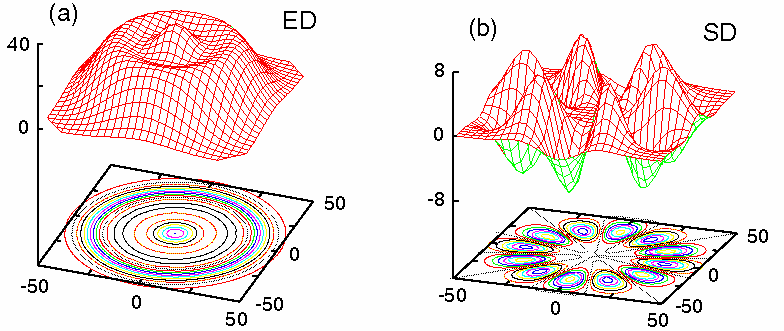
Figure 4: (Color online) UHF solution in a parabolic QD exhibiting a pure spin density wave for $N=14$, $S_{z}=0$, $R_{\rm W}=0.8$, and $B=0$. (a) The total electron density exhibiting circular symmetry; (b) The spin density exhibiting azimuthal modulation (note the 12 humps whose number is smaller than the number of electrons; on the contrary in the case of a Wigner molecule, the number of humps in the electron density is always equal to $N$). The choice of the remaining parameters is: $\hbar\omega_{0}=5$ meV and $m^{*}=0.067m_{e}$. Distances are in nanometers and the electron (ED) and spin (SD) densities in $10^{-4}$ nm^-2.

2.1.5 Unrestricted Hartree-Fock solutions representing pure spin density waves within a single quantum dot.

Another class of broken-symmetry solutions that can appear in single QDs are the spin density waves. The SDWs are unrelated to electron localization and thus are quite distinct from the Wigner molecules [20]; in single QDs, they were obtained [91] earlier within the framework of spin density functional theory. To emphasize the different nature of spin density waves and Wigner molecules, we present in figure 4 an example of a SDW obtained with the UHF approach [the corresponding parameters are: $N=14$, $S_{z}=0$, $R_{\rm W}=0.8$ ($\kappa=23.8693$), and $B=0$]. Unlike the case of Wigner molecules, the SDW exhibits a circular electron density [see figure 4(a)], and thus it does not break the rotational symmetry. Naturally, in keeping with its name, the SDW breaks the total spin symmetry and exhibits azimuthal modulations in the spin density [see figure 4(b); however, the number of humps is smaller than the number of electrons].

We mention here that the possibility of ground-state configurations with uniform electron density, but nonuniform spin density, was first discussed for 3D bulk metals using the HF method in Ref. [115].

The SDWs in single QDs appear for $R_{\rm W}\leq 1$ and are of lesser importance; thus in the following we will exclusively study the case of Wigner molecules. However, for $R_{\rm W}\leq 1$, formation of a special class of SDWs (often called electron puddles, see section 2.1.4) plays an important role in the coupling and dissociation of quantum dot molecules (see Ref. [22] and Ref. [46]).

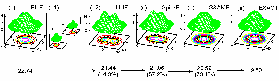
Figure 5: (Color online) Various approximation levels for the lowest singlet state of a field-free two-electron QD with $R_{W}=2.40$. The corresponding energies (in meV) are shown at the bottom of the figure. (a): Electron density of the RHF solution, exhibiting circular symmetry (due to the imposed symmetry restriction). The correlation energy $E_{\rm corr}=2.94$ meV, is defined as the difference between the energy of this state and the exact solution [shown in frame (e)]. (b1) and (b2): The two occupied orbitals (modulus square) of the symmetry-broken “singlet” UHF solution (b1), with the corresponding total electron density exhibiting non-circular shape (b2). The energy of the UHF solution shows a gain of 44.3% of the correlation energy. (c): Electron density of the spin-projected singlet (Spin-P), showing broken spatial symmetry, but with an additional gain of correlation energy. (d): the spin-and-angular-momentum projected state (S&AMP) exhibiting restored circular symmetry with a 73.1% gain of the correlation energy. The choice of parameters is: dielectric constant $\kappa=8$, parabolic confinement $\hbar\omega_{0}=5$ meV, and effective mass $m^{*}=0.067m_{e}$. Distances are in nanometers and the densities in $10^{-4}$ nm^-2.

2.2 Projection techniques and post-Hartree-Fock restoration of broken symmetries

As discussed in section 1.5, for finite systems the symmetry broken UHF solutions are only an intermediate approximation. A subsequent step of post-Hartree-Fock symmetry restoration is needed. Here we present the essentials of symmetry restoration while considering for simplicity the case of two electrons in a circular parabolic QD.

Results obtained for various approximation levels for a two-electron QD with $B=0$ and $R_{W}=2.40$ (that is, in the Wigner-molecule regime) are displayed in figure 5. In these calculations [23], the spin projection was performed following reference [31], i.e., one constructs the wave function

$$\Psi_{\rm Spin-P}(s)={\cal P}_{\rm spin}(s)\Psi_{\rm UHF},$$ (2.17)

where $\Psi_{\rm UHF}$ is the original symmetry-broken UHF determinant (which is already by construction an eigenstate of the projection $S_{z}$ of the total spin). In (2.17), the spin projection operator (projecting into a state which is an eigenstate of the square of the total spin) is given by

$${\cal P}_{\rm spin}(s)\equiv\prod_{s^{\prime}\neq s}\frac{\hat{\bf S}^{2}-s^{\prime}(s^{\prime}+1)}{s(s+1)-s^{\prime}(s^{\prime}+1)},$$ (2.18)

where the index $s^{\prime}$ runs over the quantum numbers associated with the eigenvalues $s^{\prime}(s^{\prime}+1)$ of $\hat{\bf S}^{2}$ (in units of $\hbar^{2}$), with $\hat{\bf S}$ being the total spin operator. For two electrons, the projection operator reduces to ${\cal P}_{\rm spin}^{s,t}=1\mp\varpi_{12}$, where the operator $\varpi_{12}$ interchanges the spins of the two electrons; the upper (minus) sign corresponds to the singlet ($s$ supersript), and the lower (plus) sign corresponds to the triplet ($t$ superscript) state.

The angular momentum projector (projecting into a state with total angular momentum $L$) is given by

$$2\pi{\cal P}_{L}\equiv\int_{0}^{2\pi}\rmd\gamma\exp[-\rmi\gamma(\hat{L}-L)],$$ (2.19)

where $\hat{L}=\hat{l}_{1}+\hat{l}_{2}$ is the total angular momentum operator. As seen from (2.19), application of the projection operator ${\cal P}_{L}$ to the spin-restored state $\Psi_{\rm Spin-P}(s)$ corresponds to a continuous configuration interaction expansion of the wave function that uses, however, non-orthogonal orbitals (compare section 4.1).

The application of the projection operator ${\cal P}_{L}$ to the state $\Psi_{\rm Spin-P}(s)$ generates a whole rotational band of states with good angular momenta (yrast band). The energy of the projected state with total angular momentum $L$ is given by

$$E_{\rm PRJ}(L)=\left.\int_{0}^{2\pi}h(\gamma)\rme^{\rmi\gamma L}\rmd\gamma\right/\int_{0}^{2\pi}n(\gamma)\rme^{\rmi\gamma L}\rmd\gamma,$$ (2.20)

with $h(\gamma)=\langle\Psi_{\rm Spin-P}(s;0)|{\cal H}|\Psi_{\rm Spin-P}(s;\gamma)\rangle$ and $n(\gamma)=\langle\Psi_{\rm Spin-P}(s;0)|\Psi_{\rm Spin-P}(s;\gamma)\rangle$, where $\Psi_{\rm Spin-P}(s;\gamma)$ is the spin-restored (i.e., spin-projected) wave function rotated by an azimuthal angle $\gamma$ and ${\cal H}$ is the many-body Hamiltonian. We note that the UHF energies are simply given by $E_{\rm UHF}=h(0)/n(0)$.

In the following we focus on the ground state of the two-electron system, i.e., $L=0$. The electron densities corresponding to the initial RHF approximation [shown in figure 5(a)] and the final spin-and-angular-momentum projection (S&AMP) [shown in figure 5(d)], are circularly symmetric, while those corresponding to the two intermediate approximations, i.e., the UHF and spin-projected solutions [figure 5(b2) and figure 5(c), respectively] break the circular symmetry. This behavior illustrates graphically the meaning of the term “restoration of symmetry,” and the interpretation that the UHF broken-symmetry solution refers to the intrinsic (rotating) frame of reference of the electron molecule. In light of this discussion the final projected state is called a rotating electron or (Wigner) molecule.

Expressions (2.19) and (2.20) apply directly to REMs having a single polygonal ring of $N$ localized electrons, with $\hat{L}=\sum_{i=1}^{N}{\hat{l}}_{i}$. For a generalization to electron molecules with multiple concentric polygonal rings, see section 2.2.1 below.

For restoring the total spin, an alternative method to the projection formula (2.18) can be found in the literature [33]. We do not make use of this alternative formulation in this report, but we briefly describe it here for the sake of completeness. Based on the formal similarity between the 3D angular momentum and the total spin, one can apply the formula by Peierls and Yoccoz [30] and obtain the projection operator

$${\cal P}^{s}_{{S_{z}}{q}}=\frac{2s+1}{8\pi^{2}}\int\rmd\Gamma D^{s*}_{{S_{z}}{q}}(\Gamma){\cal R}(\Gamma),$$ (2.21)

where $D^{s*}_{{S_{z}}{q}}(\Gamma)$ are the 3D Wigner $D$ functions [116], $\Gamma$ is a shorthand notation for the set of the three Euler angles $(\phi,\theta,\psi)$, and

$${\cal R}(\Gamma)=\rme^{-\rmi\phi\hat{S}_{z}}\rme^{-\rmi\theta\hat{S}_{y}}\rme^{-\rmi\psi\hat{S}_{z}}$$ (2.22)

is the rotation operator in spin space. In (2.21), the indices of the Wigner $D$ functions are $s$, $S_{z}$, and $q$.

The operator ${\cal P}^{s}_{{S_{z}}{q}}$ extracts from the symmetry broken wave function a state with a total spin $\hat{\bf S}$ and projection $S_{z}$ along the laboratory $z$ axis. However, $q$ is not a good quantum number of the many-body Hamiltonian, and the most general symmetry restored state is written as a superposition over the components of $q$, i.e.,

$$\Psi_{\rm Spin-P}(s,S_{z};i)=\sum_{q}g_{q}^{i}{\cal P}^{s}_{{S_{z}}{q}}\Psi_{\rm UHF},$$ (2.23)

where the coefficients $g_{q}^{i}$ are determined through a diagonalization of the many-body Hamiltonian in the space spanned by the nonorthogonal ${\cal P}^{s}_{{S_{z}}{q}}\Psi_{\rm UHF}$ (see also Refs. [117, 118]). In (2.23), the index $i$ reflects the possible degeneracies of spin functions with a given good total-spin quantum number $s$ [119], which is not captured by (2.18).

The Peierls-Yoccoz formulation for recovering spin-corrected wave functions applies also in the case when the UHF determinants violate in addition the conservation of spin projection [33], unlike the projector ${\cal P}_{\rm spin}(s)$ [see (2.18)] which acts on UHF determinants having a good $S_{z}=(N^{\alpha}-N^{\beta})/2$ according to the Pople-Nesbet theory presented in section 2.1.1.

In the literature [18], there are two distinguishable implementations of symmetry restoration: variation before projection (VBP) and variation after projection (VAP). In the former, which is the one that we mostly use this report, mean-field solutions with broken symmetry are first constructed and then the symmetry is restored via projection techniques as described above. In the latter, the projected wave function is used as the trial wave function directly in the variational principle (in other words the trial function is assured to have the proper symmetry).

The VAP is in general more accurate, but more difficult to implement numerically, and it has been used less often in the nuclear-physics literature. In quantum chemistry, the generalized valence bond method [120], or the spin-coupled valence bond method [121], describing covalent bonding between pairs of electrons, employ a variation after projection.

For quantum dots, the variation after projection looks promising for reducing the error of the VBP techniques in the transition region from mean-field to Wigner-molecule behavior, where this error is the largest. In fact, it has been found that the discrepancy between variation-before-projection techniques and exact solutions is systematically reduced [23, 76, 122] for stronger symmetry breaking (increasing $R_{W}$ and/or increasing magnetic field).

Moreover, in the case of an applied magnetic field (quantum dots) or a rotating trap (Bose gases), our VBP implementation corresponds to projecting cranked symmetry-unrestricted Slater determinants [123]. This is because of the “cranking” terms $-\hbar\omega_{c}L/2$ or $-\hbar\Omega L$ that contribute to the many-body Hamiltonian ${\cal H}$, respectively, with $\omega_{c}=eB/(m^{*}c)$ being the cyclotron frequency and $\Omega$ the rotational frequency of the trap; these terms arise in the single-particle component of ${\cal H}$ [see Equation (2.2) in section 2 and Equation (8.3) in section 8]. The cranking form of the many-body Hamiltonian is particularly advantageous to the variation before projection, since the cranking method provides a first-order approximation to the variation-after-projection restoration of the total angular-momentum $\hat{L}$ [124] (see also Ch 11.4.4 in Ref. [18]).

2.2.1 The REM microscopic method in medium and high magnetic field.

In our method of hierarchical approximations, we begin with a static electron molecule, described by an unrestricted Hartree-Fock determinant that violates the circular symmetry [20, 23, 25]. Subsequently, the rotation of the electron molecule is described by a post-Hartree-Fock step of restoration of the broken circular symmetry via projection techniques [22, 23, 24, 25, 26, 51, 53]. Since we focus here on the case of strong $B$, we can approximate the UHF orbitals (first step of our procedure) by (parameter free) displaced Gaussian functions; that is, for an electron localized at ${\bf R}_{j}$ ($Z_{j}$), we use the orbital [53]

$$u(z,Z_{j})=\frac{1}{\sqrt{\pi}\lambda}\exp\left(-\frac{|z-Z_{j}|^{2}}{2\lambda^{2}}-\rmi\varphi(z,Z_{j};B)\right),$$ (2.24)

with $\lambda=\tilde{l}\equiv\sqrt{\hbar/m^{*}\tilde{\omega}}$; $\tilde{\omega}=\sqrt{\omega_{0}^{2}+\omega_{c}^{2}/4}$, where $\omega_{c}=eB/(m^{*}c)$ is the cyclotron frequency and $\omega_{0}$ specifies the external parabolic confinement. We have used complex numbers to represent the position variables, so that $z=x+\rmi y$, $Z_{j}=X_{j}+\rmi Y_{j}$. The phase guarantees gauge invariance in the presence of a perpendicular magnetic field and is given in the symmetric gauge by $\varphi(z,Z_{j};B)=(xY_{j}-yX_{j})/2l_{B}^{2}$, with $l_{B}=\sqrt{\hbar c/eB}$.

For an extended 2D system, the $Z_{j}$’s form a triangular lattice [59, 125]. For finite $N$, however, the $Z_{j}$’s coincide [24, 26, 51, 52, 53] with the equilibrium positions [forming $r$ concentric regular polygons denoted as ($n_{1},n_{2},\ldots,n_{r}$)] of $N=\sum_{q=1}^{r}n_{q}$ classical point charges inside an external parabolic confinement [114]. In this notation, $n_{1}$ corresponds to the innermost ring with $n_{1}>0$. For the case of a single polygonal ring, the notation $(0,N)$ is often used; then it is to be understood that $n_{1}=N$.

The wave function of the static electron molecule is a single Slater determinant $|\Psi^{\rm{UHF}}[z]\rangle$ made out of the single-electron wave functions $u(z_{i},Z_{i})$, $i=1,\ldots,N$. Correlated many-body states with good total angular momenta $L$ can be extracted [24, 26, 51, 53] (second step) from the UHF determinant using projection operators. The projected rotating electron molecule state is given by

$$|\Phi^{\rm{REM}}_{L}\rangle=\int_{0}^{2\pi}\ldots\int_{0}^{2\pi}\rmd\gamma_{1}\ldots\rmd\gamma_{r}|\Psi^{\rm{UHF}}(\gamma_{1},\ldots,\gamma_{r})\rangle\exp\left(\rmi\sum_{q=1}^{r}\gamma_{q}L_{q}\right).$$

(2.25)

Here $L=\sum_{q=1}^{r}L_{q}$ and $|\Psi^{\rm{UHF}}[\gamma]\rangle$ is the original Slater determinant with all the single-electron wave functions of the $q$th ring rotated (collectively, i.e., coherently) by the same azimuthal angle $\gamma_{q}$. Note that (2.25) can be written as a product of projection operators acting on the original Slater determinant [i.e., on $|\Psi^{\rm{UHF}}(\gamma_{1}=0,\ldots,\gamma_{r}=0)\rangle$]. Setting $\lambda=l_{B}\sqrt{2}$ restricts the single-electron wave function in (2.24) to be entirely in the lowest Landau level (see Appendix in Ref. [53]). The continuous-configuration-interaction form of the projected wave functions [i.e., the linear superposition of determimants in (2.25)] implies a highly entangled state. We require here that $B$ is sufficiently strong so that all the electrons are spin-polarized and that the ground-state angular momentum $L\geq L_{0}\equiv\sum_{i=0}^{N-1}i=N(N-1)/2$ (or equivalently that the fractional filling factor $\nu\equiv L_{0}/L\leq 1$). The state corresponding to $L_{0}$ is a single Slater determinant in the lowest Landau level and is called the “maximum density droplet” [126]. For high $B$, the calculations in this paper do not include the Zeeman contribution, which, however, can easily be added (for a fully polarized dot, the Zeeman contribution to the total energy is $Ng^{*}\mu_{B}B/2$, with $g^{*}$ being the effective Landé factor and $\mu_{B}$ the Bohr magneton).

Due to the point-group symmetries of each polygonal ring of electrons in the UHF wave function, the total angular momenta $L$ of the rotating crystalline electron molecule are restricted to the so-called magic angular momenta, i.e.,

$$L_{m}=L_{0}+\sum_{q=1}^{r}k_{q}n_{q},$$ (2.26)

where the $k_{q}$’s are non-negative integers (when $n_{1}=1$, $k_{1}=0$).

Magic angular momenta associated with multiple rings have been discussed in Refs. [24, 26, 51, 52, 53]. For the simpler cases of $(0,N)$ or $(1,N-1)$ rings, see, e.g., Ref. [127] and Ref. [128].

The partial angular momenta associated with the $q$th ring, $L_{q}$ [see (2.25)], are given by

$$L_{q}=L_{0,q}+k_{q}n_{q},$$ (2.27)

where $L_{0,q}=\sum_{i=i_{q}+1}^{i_{q}+n_{q}}(i-1)$ with $i_{q}=\sum_{s=1}^{q-1}n_{s}$ $(i_{1}=0)$, and $L_{0}=\sum_{q=1}^{r}L_{0,q}$.

The energy of the REM state (2.25) is given [24, 51, 52, 53] by

$$E^{\rm{REM}}_{L}=\left.{\int_{0}^{2\pi}h([\gamma])\rme^{\rmi[\gamma]\cdot[L]}\rmd[\gamma]}\right/{\int_{0}^{2\pi}n([\gamma])\rme^{\rmi[\gamma]\cdot[L]}\rmd[\gamma]},$$ (2.28)

with the Hamiltonian and overlap matrix elements $h([\gamma])=\langle\Psi^{\rm{UHF}}([0])|{\cal H}|\Psi^{\rm{UHF}}([\gamma])\rangle$ and $n([\gamma])=\langle\Psi^{\rm{UHF}}([0])|\Psi^{\rm{UHF}}([\gamma])\rangle$, respectively, and $[\gamma]\cdot[L]=\sum_{q=1}^{r}\gamma_{q}L_{q}$. The UHF energies are simply given by $E_{\rm{UHF}}=h([0])/n([0])$.

The crystalline polygonal-ring arrangement $(n_{1},n_{2},\ldots,n_{r})$ of classical point charges is portrayed directly in the electron density of the broken-symmetry UHF, since the latter consists of humps centered at the localization sites $Z_{j}$’s (one hump for each electron). In contrast, the REM has good angular momentum and thus its electron density is circularly uniform. To probe the crystalline character of the REM, we use the conditional probability distribution (CPD) defined in (1.1). $P({\bf r},{\bf r}_{0})$ is proportional to the conditional probability of finding an electron at ${\bf r}$, given that another electron is assumed at ${\bf r}_{0}$. This procedure subtracts the collective rotation of the electron molecule in the laboratory frame of referenece, and, as a result, the CPDs reveal the structure of the many body state in the intrinsic (rotating) reference frame.

2.2.2 Group structure and sequences of magic angular momenta.

It has been demonstrated [25] that the broken-symmetry UHF determinants and orbitals describe 2D electronic molecular stuctures (Wigner molecules) in close analogy with the case of natural 3D molecules. However, the study of Wigner molecules at the UHF level restricts their description to the intrinsic (nonrotating) frame of reference. Motivated by the case of natural atoms, one can take a subsequent step and address the properties of collectively rotating Wigner molecules in the laboratory frame of reference. As is well known, for natural atoms, this step is achieved by writing the total wave function of the molecule as the product of the electronic and ionic partial wave functions. In the case of the purely electronic Wigner molecules, however, such a product wave function requires the assumption of complete decoupling between intrinsic and collective degrees of freedom, an assumption that might be justifiable in limiting cases only. The simple product wave function was used in earlier treatments of Wigner molecules; see, e.g., Ref.  [128]. The projected wave functions employed here are integrals over such product wave functions, and thus they account for quantal fluctuations in the rotational degrees of freedom. The reduction of the projected wave functions to the limiting case of a single product wave function is discussed in Ch 11.4.6.1 of Ref. [18].

As was discussed earlier, in the framework of the broken-symmetry UHF solutions, a further step is needed – and this companion step can be performed by using the post-Hartree-Fock method of restoration of broken symmetries via projection techniques (see section 2.2). In this section, we use this approach to illustrate through a couple of concrete examples how certain universal properties of the exact solutions, i.e., the appearance of magic angular momenta [127, 128, 129, 130, 131, 132, 133] in the exact rotational spectra, relate to the symmetry broken UHF solutions. Indeed, we demonstrate that the magic angular momenta are a direct consequence of the symmetry breaking at the UHF level and that they are determined fully by the molecular symmetries of the UHF determinant.

Figure 6: (Color online) The UHF solution exhibiting breaking of the circular symmetry for $N=3$ and $S_{z}=1/2$ at $R_{W}=10$ and $B=0$. (a-b): real orbitals for the two spin-up electrons. (c): real orbital for the single spin-down electron. (d): total electron density (ED). (e): spin density (SD, difference of the spin-up minus the spin-down partial electron densities). The choice of the remaining parameters is: $\hbar\omega_{0}=5$ meV and $m^{*}=0.067m_{e}$. Distances are in nanometers. The real orbitals are in 10^-3 nm^-1 and the densities (electron density and spin density) in 10^-4 nm^-2. The arrows indicate the spin direction.

As an illustrative example, we have chosen the relatively simple, but non trivial case, of $N=3$ electrons. For $B=0$, both the $S_{z}=1/2$ and $S_{z}=3/2$ polarizations can be considered. We start with the $S_{z}=1/2$ polarization, whose broken-symmetry UHF solution [25] is portayed in figure 6 and which exhibits a breaking of the total spin symmetry in addition to the rotational symmetry. Let us denote the corresponding UHF determinant [made out of the three spin orbitals in figure 6(a), figure 6(b), and figure 6(c)] as $|\downarrow\uparrow\uparrow\rangle$. We first proceed with the restoration of the total spin by noticing that $|\downarrow\uparrow\uparrow\rangle$ has a lower point-group symmetry (see Ref. [25]) than the $C_{3v}$ symmetry of an equilateral triangle. The $C_{3v}$ symmetry, however, can be readily restored by applying the projection operator (2.19) to $|\downarrow\uparrow\uparrow\rangle$ and by using the character table of the cyclic $C_{3}$ group (see Table I in Ref. [25]). Then for the intrinsic part of the many-body wave function, one finds two different three-determinantal combinations, namely

$$\Phi_{\rm{intr}}^{E^{\prime}}(\gamma_{0})=|\downarrow\uparrow\uparrow\rangle+\rme^{2\pi\rmi/3}|\uparrow\downarrow\uparrow\rangle+\rme^{-2\pi\rmi/3}|\uparrow\uparrow\downarrow\rangle,$$ (2.29)

and

$$\Phi_{\rm{intr}}^{E^{\prime\prime}}(\gamma_{0})=|\downarrow\uparrow\uparrow\rangle+\rme^{-2\pi\rmi/3}|\uparrow\downarrow\uparrow\rangle+\rme^{2\pi\rmi/3}|\uparrow\uparrow\downarrow\rangle,$$ (2.30)

where $\gamma_{0}=0$ denotes the azimuthal angle of the vertex of the equilateral triangle associated with the original spin-down orbital in $|\downarrow\uparrow\uparrow\rangle$. We note that, unlike the intrinsic UHF Slater determinant, the intrinsic wave functions $\Phi_{\rm{intr}}^{E^{\prime}}$ and $\Phi_{\rm{intr}}^{E^{\prime\prime}}$ here are eigenstates of the square of the total spin operator ${\hat{\bf S}}^{2}$ ($\hat{\bf S}=\sum_{i=1}^{3}\hat{\bf s}_{i}$) with quantum number $s=1/2$. This can be verified directly by applying ${\hat{\bf S}}^{2}$ to them.

To restore the circular symmetry in the case of a (0,N) ring arrangement, one applies the projection operator (2.19). Note that the operator ${\cal P}_{L}$ is a direct generalization of the projection operators for finite point-groups discussed in Ref. [25] to the case of the continuous cyclic group $C_{\infty}$ [the phases $\exp(i\gamma L)$ are the characters of $C_{\infty}$].

The symmetry-restored projected wave function, $\Psi_{\rm{PRJ}}$, (having both good total spin and angular momentum quantum numbers) is of the form,

$$2\pi\Psi_{\rm{PRJ}}=\int^{2\pi}_{0}\rmd\gamma\Phi_{\rm{intr}}^{E}(\gamma)\rme^{\rmi\gamma L},$$ (2.31)

where now the intrinsic wave function [given by (2.29) or (2.30)] has an arbitrary azimuthal orientation $\gamma$. We note that, unlike the phenomenological Eckardt-frame model [128, 132] where only a single product term is involved, the PRJ wave function in (2.31) is an average over all azimuthal directions over an infinite set of product terms. These terms are formed by multiplying the intrinsic part $\Phi_{\rm{intr}}^{E}(\gamma)$ with the external rotational wave function $\exp(i\gamma L)$ (the latter is properly characterized as “external”, since it is an eigenfunction of the total angular momentum $\hat{L}$ and depends exclusively on the azimuthal coordinate $\gamma$).

The operator ${\hat{R}(2\pi/3)\equiv\exp(-\rmi 2\pi{\hat{L}}/3})$ can be applied onto $\Psi_{\rm{PRJ}}$ in two different ways, namely either on the intrinsic part $\Phi_{\rm{intr}}^{E}$ or the external part $\exp(\rmi\gamma L)$. Using (2.29) and the property $\hat{R}(2\pi/3)\Phi_{\rm{intr}}^{E^{\prime}}=\exp(-2\pi\rmi/3)\Phi_{\rm{intr}}^{E^{\prime}}$, one finds,

$$\hat{R}(2\pi/3)\Psi_{\rm{PRJ}}=\exp(-2\pi\rmi/3)\Psi_{\rm{PRJ}},$$ (2.32)

from the first alternative, and

$$\hat{R}(2\pi/3)\Psi_{\rm{PRJ}}=\exp(-2\pi L\rmi/3)\Psi_{\rm{PRJ}},$$ (2.33)

from the second alternative. Now if $\Psi_{\rm{PRJ}}\neq 0$, the only way that equations (2.32) and (2.33) can be simultaneously true is if the condition $\exp[2\pi(L-1)\rmi/3]=1$ is fulfilled. This leads to a first sequence of magic angular momenta associated with total spin $s=1/2$, i.e.,

$$L=3k+1,\;k=0,\pm 1,\pm 2,\pm 3,\ldots$$ (2.34)

Using (2.30) for the intrinsic wave function, and following similar steps, one can derive a second sequence of magic angular momenta associated with good total spin $s=1/2$, i.e.,

$$L=3k-1,\;k=0,\pm 1,\pm 2,\pm 3,\ldots$$ (2.35)

Figure 7: (Color online) The UHF case exhibiting breaking of the circular symmetry for $N=3$ and $S_{z}=3/2$ at $R_{W}=10$ and $B=0$. (a-c): real orbitals. (d): the corresponding electron density (ED). The choice of the remaining parameters is: $\hbar\omega_{0}=5$ meV and $m^{*}=0.067m_{e}$. Distances are in nanometers. The real orbitals are in 10^-3 nm^-1 and the total electron density in 10^-4 nm^-2. The arrows indicate the spin direction.

In the fully spin-polarized case, the UHF determinant is portrayed in figure 7. This UHF determinant, which we denote as $|\uparrow\uparrow\uparrow\;\rangle$, is already an eigenstate of $\hat{\bf S}^{2}$ with quantum number $s=3/2$. Thus only the rotational symmetry needs to be restored, that is, the intrinsic wave function is simply $\Phi^{A}_{\rm{intr}}(\gamma_{0})=|\uparrow\uparrow\uparrow\;\rangle$. Since $\hat{R}(2\pi/3)\Phi^{A}_{\rm{intr}}=\Phi^{A}_{\rm{intr}}$, the condition for the allowed angular momenta is $\exp[-2\pi L\rmi/3]=1$, which yields the following magic angular momenta,

$$L=3k,\;k=0,\pm 1,\pm 2,\pm 3,\ldots$$ (2.36)

We note that in high magnetic fields only the fully polarized case is relevant and that only angular momenta with $k>0$ enter in (2.36) (see Ref. [24]). In this case, in the thermodynamic limit, the partial sequence with $k=2q+1$, $q=0,1,2,3,\ldots$ is directly related to the odd filling factors $\nu=1/(2q+1)$ of the fractional quantum Hall effect [via the relation $\nu=N(N-1)/(2L)$]. This suggests that the observed hierarchy of fractional filling factors in the quantum Hall effect may be viewed as a signature originating from the point group symmetries of the intrinsic wave function $\Phi_{\rm{intr}}$, and thus it is a manifestation of symmetry breaking at the UHF mean-field level.

We further note that the discrete rotational (and more generally rovibrational) collective spectra associated with symmetry-breaking in a QD may be viewed as finite analogs to the Goldstone modes accompanying symmetry breaking transitions in extended media (see Ref. [10]). Recently there has been some interest in studying Goldstone-mode analogs in the framework of symmetry breaking in trapped BECs with attractive interactions [88].

2.3 The symmetry breaking dilemma and density functional theory

Density functional theory (and its extension for cases with a magnetic field known as current density functional theory) was initially considered [3] (and was extensively applied [3, 92, 94]) as a promising method for studying 2D semiconductor QDs. However, it soon became apparent [22, 23, 25, 46] that density functional approaches exhibited severe drawbacks when applied to the regime of strong correlations in QDs, where the underlying physics is associated with symmetry breaking leading to electron localization and formation of Wigner molecules. The inadequacies of density functional approaches in the field of QDs have by now gained broad recognition [41, 134, 135].

In particular, unlike the Hartree-Fock case for which a consistent theory for the restoration of broken symmetries has been developed (see, e.g., the earlier Refs. [18, 30, 31, 32, 33]; for developments in the area of quantum dots, see the more recent Refs. [22, 23, 24, 25, 46]), the breaking of space symmetry within the spin-dependent density functional theory poses [136] a serious dilemma. This dilemma has not been resolved [137] to date; several remedies are being proposed, but none of them appears to be completely devoid of inconsistencies. In particular, a theory for symmetry restoration of broken-symmetry solutions [134, 135] within the framework of density functional theory has not been developed as yet. This puts the density functional methods in a clear disadvantage with regard to the modern fields of quantum information and quantum computing; for example, the description of quantum entanglement (see section 5.1.4 below) requires the ability to calculate many-body wave functions exhibiting good quantum numbers, and thus it lies beyond the reach of density functional theory.

Moreover, due to the unphysical self-interaction error, the density-functional theory becomes erroneously more resistant to space symmetry breaking [138] compared to the UHF (which is free from such an error), and thus it fails to describe a whole class of broken symmetries involving electron localization, e.g., the formation at $B=0$ of Wigner molecules in quantum dots [20, 46] and in thin quantum wires [139], the hole trapping at Al impurities in silica [140], or the interaction driven localization-delocalization transition in $d$- and $f$- electron systems, like Plutonium [141].

Recently, the shortcomings of the density functional theory to properly describe magnetic phenomena (such as exchange coupling constants associated with symmetry breaking of the total spin) has attracted significant attention in the quantum chemistry literature (see, e.g., Refs. [142, 143, 144]).

2.4 More on symmetry restoration methods

In the framework of post-Hartree-Fock hierarchical approximations, projection techniques are one of methods used to treat correlations beyond the unrestricted Hartree-Fock. Two other methods are briefly discussed in this section, i.e., the method of symmetry restoration via random phase approximation (RPA) and the generator coordinate method (GCM).

2.4.1 Symmetry restoration via random phase approximation.

This method introduces energy correlations by considering the effect of the zero-point motion of normal vibrations associated with the small amplitude motion of the time-dependent-Hartree-Fock mean field (which is equivalent to the RPA). In the case of space symmetry breaking, one of the RPA vibrational frequencies vanishes, and the corresponding motion is associated with the rotation of the system as a whole (rotational Goldstone mode), with a moment of inertia given by the so-called Thouless-Valatin expression [145].

The method has been used to calculate correlation energies of atomic nuclei [146, 147] and most recently to restore the broken symmetry in circular quantum dots [148] (mainly for the case of two electrons at zero magnetic field). As discussed in Ref. [148], restoration of the total spin cannot be treated within RPA.

2.4.2 The generator coordinate method.

The projection techniques by themselves do not take into account quantum correlation effects arising from the vibrations and other large-amplitude intrinsic collective distortions of the Wigner molecule. For the inclusion of the effects of such collective motions, a natural extension beyond projection techniques is the generator coordinate method (see Ch 10 in Ref. [18]). Unlike the RPA, the GCM can treat large-amplitude collective motion in combination with the retoration of the total spin. Indeed, it has been shown that the RPA harmonic vibrations are a limiting small-amplitude case of the large-amplitude collective motion described via the generator coordinate method [18].

The GCM represents an additional step in the hierarchy of approximations described in section 1.5 and its use will result in a further reduction of the difference from the exact solutions. The GCM is complicated and computationally more expensive compared to projection techniques. Recent computational advances, however, have allowed rather extensive applications of the method in nuclear physics (see, e.g., Ref. [38]). As yet, applications of the GCM to quantum dots or trapped atomic gases have not been reported.

The GCM employs a very general form for the trial many-body wave functions expressed as a continuous superposition of determinants $|\Psi[a]\rangle$ (or permanents for bosons), i.e.,

$$|\Phi\rangle=\int\rmd[a]f[a]|\Psi[a]\rangle,$$ (2.37)

where $[a]=(a_{1},a_{2},\ldots,a_{k})$ is a set of collective parameters depending on the physics of the system under consideration. An example of such parameters are the azimuthal angles $(\gamma_{1},\gamma_{2},\ldots,\gamma_{r})$ in the REM trial wave function (2.25). Of course the crucial difference between the REM wave function (2.25) and the general GCM function (2.37) is the fact that the weight coefficients $f[a]$ in the former are known in advance (they coincide with the characters of the underlying symmetry group), while in the latter they are calculated numerically via the Hill-Wheeler-Griffin equations [149, 150]

$$\int\rmd[a^{\prime}]h(a,a^{\prime})f[a^{\prime}]=E\int\rmd[a^{\prime}]n(a,a^{\prime})f[a^{\prime}],$$ (2.38)

where $E$ are the eigenenergies, and

$$h(a,a^{\prime})=\langle\Psi[a]|{\cal H}|\Psi[a^{\prime}]\rangle,$$ (2.39)

$$n(a,a^{\prime})=\langle\Psi[a]|\Psi[a^{\prime}]\rangle$$ (2.40)

are the Hamiltonian and overlap kernels. The Hill-Wheeler-Griffin equation (2.38) is usually solved numerically by discretization; then one can describe it as a diagonalization of the many-body hamiltonian in a nonorthogonal basis formed with the determinants $|\Psi[a]\rangle$.

An example of a potential case for the application of the GCM is an anisotropic quamtum dot ($\zeta<1$, with $\zeta=\omega_{x}/\omega_{y}$) In this case, one cannot use projection techniques to restore the total angular momentum, since the external confinement does not possess circular symmetry. Application of the GCM, however, will produce numerical values for the expansion coefficients $f[\gamma]$, and these values will reduce to $\exp[\rmi\sum_{q=1}^{r}\gamma_{q}L_{q}]$ for the circular case $\zeta=1$ [while the GCM wave function will reduce to the REM wave function (2.25)]. It is apparent that the GCM many-body wave function changes continuously with varying anisotropy $\zeta$, although the symmetry properties of the confinement potential change in an abrupt way at the point $\zeta\rightarrow 1$.

3 Symmetry breaking and subsequent symmetry restoration for neutral and charged bosons in confined geometries: Theoretical framework

3.1 Symmetry breaking for bosons, Gross-Pitaevskii wave functions, and permanents

Mean-field symmetry breaking for bosonic systems is transparent in the context of two-component condensates, where each species is necessarily associated with a different space orbital [151, 152]. For one species of bosons, symmetry breaking can be considered through a generalization of the UHF method of different orbitals for different spins known from the case of electrons in quantum chemistry and in quantum dots (section 2.1.1). Indeed, as shown in Refs. [60, 63, 153], one can allow each bosonic particle to occupy a different orbital $\phi_{i}({\bf r}_{i})$. Then the permanent $|\Phi_{N}\rangle={\rm Perm}[\phi_{1}({\bf r}_{1}),\ldots,\phi_{N}({\bf r}_{N})]$ serves as the many-body wave function of an unrestricted Bose-Hartree-Fock (UBHF) approximation. This wave function reduces to the Gross-Pitaevskii form with the restriction that all bosons occupy the same orbital $\phi_{0}({\bf r})$, i.e., $|\Phi^{\rm{GP}}_{N}\rangle=\prod_{i=1}^{N}\phi_{0}({\bf r}_{i})$, and $\phi_{0}({\bf r})$ is determined self-consistently at the restricted Bose-Hartree-Fock (RBHF) level via the equation [154]

$$[H_{0}({\bf r}_{1})+(N-1)\int d{\bf r}_{2}\phi^{*}_{0}({\bf r}_{2})v({\bf r}_{1},{\bf r}_{2})\phi_{0}({\bf r}_{2})]\phi_{0}({\bf r}_{1})=\varepsilon_{0}\phi_{0}({\bf r}_{1}).$$ (3.1)

Here $v({\bf r}_{1},{\bf r}_{2})$ is the two-body repulsive interaction, which is taken to be a contact potential, $v_{\delta}=g\delta({\bf r}_{1}-{\bf r}_{2})$, for neutral bosons, or the Coulomb repulsion $v_{C}=e^{2}Z^{2}/(\kappa|{\bf r}_{1}-{\bf r}_{2}|)$ for charged bosons. The single-particle Hamiltonian is given by

$$H_{0}({\bf r})=-\hbar^{2}\nabla^{2}/(2m)+m\omega_{0}^{2}{\bf r}^{2}/2,$$ (3.2)

where $\omega_{0}$ characterizes the circular harmonic confinement, and where we have considered a non-rotating trap.

Compared to the fermionic case (see section 2.1.1), the self-consistent determination of the UBHF orbitals is rather complicated and numerically highly demanding (see section 2.5.3 in Ref. [155]). In fact, the self-consistent UHBF equations cannot be put into a standard (canonical) eigenvalue-problem form due to two reasons:(i) unitary transformations cannot be used to simplify the equations, since the permanent of the product of two matrices does not factorize into a product of two simpler terms (unlike the electronic case where the determinant of the product of two matrices is equal to the product of the corresponding determinants) and (ii) as a result of boson statistics, the bosonic orbitals cannot be assumed to be (and remain) orthogonal, which leads to additional coupling terms between the non-orthogonal orbitals.

In the literature [156], an attempt has been made to derive unrestricted self-consistent equations for bosons by disregarding point (ii) mentioned above and invoking the assumption of orthonormal orbitals. Such equations of course are not of general validity, although they appear to be useful for describing fragmentation of Bose condensates in double wells.

The difficulties of the self-consistent treatment can be bypassed and the UBHF problem can be simplified through consideration of explicit analytic expressions for the space orbitals $\phi_{i}({\bf r}_{i})$. In particular, for repulsive interactions, the bosons must avoid each other in order to minimize their mutual repulsion, and thus, in analogy with the case of electrons in QDs, one can take all the orbitals to be of the form of displaced Gaussians, namely,

$$\phi_{i}({\bf r}_{i})=\pi^{-1/2}\sigma^{-1}\exp[-({\bf r}_{i}-{\bf a}_{i})^{2}/(2\sigma^{2})].$$ (3.3)

The positions ${\bf a}_{i}$ describe the vertices of concentric regular polygons, with both the width $\sigma$ and the radius $a=|{\bf a}_{i}|$ of the regular polygons determined variationally through minimization of the total energy

$$E_{\rm{UBHF}}=\langle\Phi_{N}|{\cal H}|\Phi_{N}\rangle/\langle\Phi_{N}|\Phi_{N}\rangle,$$ (3.4)

where

$${\cal H}=\sum_{i=1}^{N}H_{0}({\bf r}_{i})+\sum_{i<j}^{N}v({\bf r}_{i},{\bf r}_{j})$$ (3.5)

is the many-body Hamiltonian.

With the above choice of localized orbitals the unrestricted permanent $|\Phi_{N}\rangle$ breaks the continuous rotational symmetry. However, the resulting energy gain becomes substantial for stronger repulsion. Controlling this energy gain (the strength of correlations) is the ratio $R_{\delta}$ (or $R_{W}$) between the strength of the repulsive potential and the zero-point kinetic energy. Specifically, for a 2D trap, one has

$$R_{\delta}=gm/(2\pi\hbar^{2})$$ (3.6)

for a contact potential (for $R_{W}$, see section 2.1.2). Note that in this section, we refer to the case of a non-rotating trap; the generalization to rotating traps is presented later in section 8.

3.2 Repelling bosons in harmonic traps: Restoration of broken symmetry.

Although the optimized UBHF permanent $|\Phi_{N}\rangle$ performs very well regarding the total energies of the trapped bosons, in particular in comparison to the resctricted wave functions (e.g., the GP anzatz), it is still incomplete. Indeed, due to its localized orbitals, $|\Phi_{N}\rangle$ does not preserve the circular (rotational) symmetry of the 2D many-body Hamiltonian $H$. Instead, it exhibits a lower point-group symmetry, i.e., a $C_{2}$ symmetry for $N=2$ and a $C_{5}$ one for the $(1,5)$ structure of $N=6$ (see section 8 below). As a result, $|\Phi_{N}\rangle$ does not have a good total angular momentum. In analogy with the case of electrons in quantum dots, this paradox is resolved through a post-Hartree-Fock step of restoration of broken symmetries via projection techniques [23, 24, 25, 60], yielding a new wave function $|\Psi_{N,L}^{\rm{PRJ}}\rangle$ with a definite angular momentum $L$, that is

$$2\pi|\Psi_{N,L}^{\rm{PRJ}}\rangle=\int^{2\pi}_{0}\rmd\gamma|\Phi_{N}(\gamma)\rangle\rme^{\rmi\gamma L},$$ (3.7)

where $|\Phi_{N}(\gamma)\rangle$ is the original UBHF permanent having each localized orbital rotated by an azimuthal angle $\gamma$, with $L$ being the total angular momentum. The projection yields wave functions for a whole rotational band. Note that the projected wave function $|\Psi_{N,L}^{\rm{PRJ}}\rangle$ in (3.7) may be regarded as a superposition of the rotated permanents $|\Phi_{N}(\gamma)\rangle$, thus corresponding to a “continuous-configuration-interaction” solution.

The energies of the projected states are given by

$$E_{L}^{\rm{PRJ}}=\langle\Psi_{N,L}^{\rm{PRJ}}|{\cal H}|\Psi_{N,L}^{\rm{PRJ}}\rangle/\langle\Psi_{N,L}^{\rm{PRJ}}|\Psi_{N,L}^{\rm{PRJ}}\rangle.$$ (3.8)

4 Other many-body methods

4.1 Exact diagonalization methods: Theoretical framework

We will discuss the essential elements of the exact-diagonalization method here by considering the special, but most important case of a many-body Hilbert space defined via the restriction that the single-particle states belong exclusively to the lowest Landau level. For 2D electrons, this LLL restriction is appropriate in the case of very high $B$. For rotating bosons in a harmonic trap, the LLL restriction is appropriate for $\Omega\sim\omega_{0}$ and a very weak repulsive contact potential. The particulars of the EXD method for quantum dots in the case of field-free (and/or low $B$) conditions will be discussed below in section 5.1.2.

For sufficiently high magnetic field values (i.e., in the fractional quantum Hall effect, regime), the electrons are fully spin-polarized and the Zeeman term (not shown here) does not need to be considered. In the $B\rightarrow\infty$ limit, the external confinement $V(x,y)$ can be neglected, and the many-body $H$ can be restricted to operate in the lowest Landau level, reducing to the form [24, 26, 52, 53]

$${\cal H}_{\rm LLL}=N\frac{\hbar\omega_{c}}{2}+\sum_{i=1}^{N}\sum_{j>i}^{N}\frac{e^{2}}{\kappa r_{ij}},$$ (4.1)

where $\omega_{c}=eB/(m^{*}c)$ is the cyclotron frequency. Namely, one needs to diagonalize the interaction Hamiltonian only.

For the case of rotating bosons in the LLL, one needs to replace in (4.1) the Coulomb interaction by $g\delta({\bf r}_{i}-{\bf r}_{j})$ and the cyclotron frequency by $2\Omega$ (see the Appendix for the details of the equivalence between magnetic field $B$ and rotational frequency $\Omega$; in short $\omega_{c}\rightarrow 2\Omega$).

For a given total angular momentum $L=\sum_{k=1}^{N}l_{k}$, the exact-diagonalization $N$-body wave function is a linear superposition of Slater determinants for fermions (or permanents for bosons) $\Psi(J)$ made out of lowest-Landau-level single-particle wave functions (see the Appendix),

$$\phi_{l}(z)=\frac{1}{\Lambda\sqrt{\pi l!}}\left(\frac{z}{\Lambda}\right)^{l}e^{-zz^{*}/(2\Lambda^{2})},$$ (4.2)

where $\Lambda=\sqrt{2\hbar c/(eB)}=l_{B}\sqrt{2}$ for the case of electrons in QDs ($l_{B}$ being the magnetic length), and $\Lambda=\sqrt{\hbar/(m\omega_{0})}$ for the case of bosons in rotating traps. In (4.2), we used complex coordinates $z=x+\rmi y$, instead of the usual vector positions ${\bf r}=(x,y)$; below we will use either notation interchangeably as needed.

Thus, the many-body EXD wave function is written as

$$\Phi^{\rm EXD}(z_{1},z_{2},\ldots,z_{N})=\sum_{J=1}^{K}C_{J}\Psi(J)$$ (4.3)

with the index $J$ denoting any set of $N$ single-particle angular momenta $\{l_{1},l_{2},\ldots,l_{N}\}$ such that

$$l_{1}<l_{2}<\ldots<l_{N}$$ (4.4)

for fermions and

$$l_{1}\leq l_{2}\leq\ldots\leq l_{N}$$ (4.5)

for bosons, the absence or presence of the equal signs being determined by the different statistics between fermions and bosons, respectively.

Using the expansion (4.3), one transforms the many-body Schrödinger equation

$${\cal H}\Phi^{\rm EXD}(z_{1},z_{2},\ldots,z_{N})=E\Phi^{\rm EXD}(z_{1},z_{2},\ldots,z_{N}),$$ (4.6)

into a matrix eigenvalue problem. When the single-particle states are orthonormal [like the LLL ones in (4.2)], the matrix elements $\langle\Psi(I)|{\cal H}|\Psi(J)\rangle$ between two Slater determinants are calculated using the so-called Slater rules (see, e.g., Ch 2.3.3 of Ref. [19]). For the case of bosons, the correpsonding rules for the matrix elements $\langle\Psi(I)|{\cal H}|\Psi(J)\rangle$ between two permanents are given in the appendix of Ref. [72].

We remark here that the calculation of energies associated with projected wave functions [see, e.g., Equation (3.8)] requires calculation of similar matrix elements between two Slater determinants (or permanents) with non-orthogonal orbitals; the corresponding formulas for the case of fermions can be found in Ch 6.3. of Ref. [157], and for the case of bosons in Ref. [155].

Of course a necessary ingredient for the application of the above rules is the knowledge of the matrix elements of the two-body interaction $v({\bf r}_{1},{\bf r}_{2})$, i.e.,

$$v_{\alpha\beta\gamma\Delta}\equiv\int\rmd{\bf r}_{1}\rmd{\bf r}_{2}\phi^{*}_{\alpha}(1)\phi^{*}_{\beta}(2)v(1,2)\phi_{\gamma}(1)\phi_{\Delta}(2).$$ (4.7)

In the general case, these two-body matrix elements need to be calculated numerically. For the simpler case specified by the LLL orbitals (4.2), the two-body matrix elements are given by analytic expressions. In particular, for the Coulomb repulsion, see Refs. [26, 158]; for a contact potential, see Ref. [159].

The dimension ${\cal D}$ of the Hilbert space increases very fast with the number of particles $N$ and the value of the total angular momentum $L$, and is is controlled by the maximum allowed single-particle angular momentum $l_{\rm{max}}$, such that $l_{k}\leq l_{\rm{max}}$, $1\leq k\leq N$. By varying $l_{\rm{max}}$, we can check that this choice produces well converged numerical results.

For the solution of the large scale, but sparse, EXD matrix eigenvalue problem associated with the special Hamiltonian $H_{\rm{LLL}}$ [or the general one in (2.1)], we use the ARPACK computer code [160].

The availabilty of analytic expressions for the two-body interaction has greatly facilitated exact-diagonalization calculations in the lowest Landau level (appropriate for quantum dots at high $B$), and in this case (starting with Refs. [26, 161]) diagonalization of large matrices of dimensions of order 500,000 x 500,000 has become a commom occurrence. For circular quantum dots, similar analytic expressions for the matrix elements of the Coulomb interaction between general Darwin-Fock orbitals [162, 163] (i.e., the single-particle orbitals of a circular 2D harmonic oscillator under a perpendicular magnetic field $B$) are also available [129, 164], but they are not numerically as stable as Tsiper’s expressions [158] in the lowest Landau level.

Exact-diagonalization calculations for field-free (and/or low $B$) conditions have been presented in several papers. Among them, we note the exact-diagonalization calculations of Refs. [77, 97, 165, 166, 167, 168, 169, 170]. EXD calculations employing Coulombic two-body matrix elements that are calculated numerically have also been reported for elliptic quantum dots (see section 5.1.2 below). Furthermore, some authors have used the method of hyperspherical harmonics [171] for circular quantum dots, while others have carried out exact-diagonalization calculations for quantum dots with a polygonal external confinement [172].

Concerning EXD calculations in the lowest Landau level, we mention Refs. [26, 95, 128, 129, 130, 131, 132, 173, 174, 175, 176] for the case of quantum dots (high $B$) and Refs. [67, 68, 69, 72, 177, 178] for the case of bosons in rapidly rotating traps. A version of EXD in the LLL uses a correlated basis constructed out of composite-fermion wave functions [176], while another exact-diagonalization version used non-orthogonal floating Gaussians in the place of the usual single-particle states (4.2) in the LLL.

For two electrons in a single quantum dot, exact calculations have been carried out through separation into center-of-mass and relative coordinates [50, 179, 180]. In addition, EXD calculations have been reported for two electrons in a double quantum dot [89, 181].

It is of interest to note that the EXD approach is also used in other fields, but under different names. In particular, the term “shell model calculations” is used in nuclear theory, while the term “full configuration interaction” is employed in quantum chemistry.

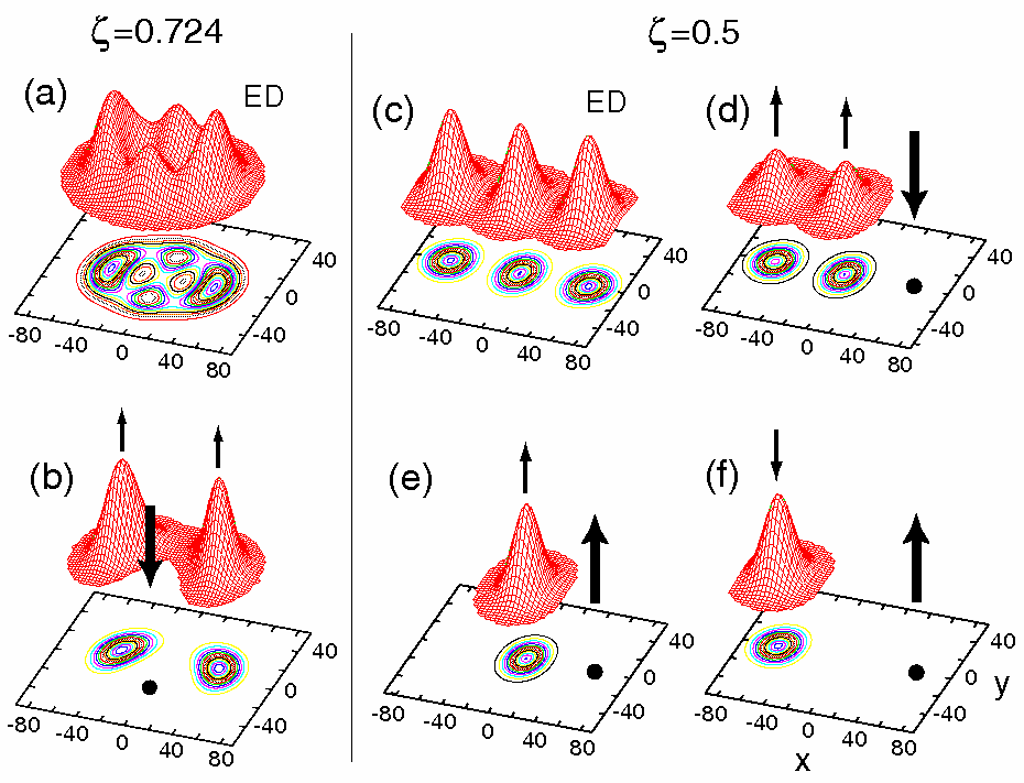
Figure 8: (Color online) Exact-diagonalization electron densities (EDs) and spin-resolved CPDs for $N=3$ electrons in an anisotropic quantum dot at zero magnetic field ($B=0$) and in the case of a strong Coulomb repulsion with a dielectric constant $\kappa=1$. (a-b) Results for the ground state (which has total spin $s=1/2$ and spin projection $S_{z}=1/2$) when $\hbar\omega_{x}=4.23$ meV and $\hbar\omega_{y}=5.84$ meV (i.e., for an intermediate anisotropy $\zeta=0.724$). (c-f) Results for the first excited state (which has also total spin $s=1/2$ and spin projection $S_{z}=1/2$) when $\hbar\omega_{x}=3.137$ meV and $\hbar\omega_{y}=6.274$ meV (i.e., for a strong anisotropy $\zeta=0.5$). The thick arrows and solid dots in the CPDs indicate the spin direction $\sigma_{0}$ and position ${\bf r}_{0}$ of the fixed electron [see (1.2)]. The thin arrows indicate the spin direction of the remaining two electrons. The effective mass is $m^{*}=0.070m_{e}$ for the intermediate anisotropy (a-b) and $m^{*}=0.067m_{e}$ for the strong anisotropy (c-f). Lengths are in nanometers. The vertical axes are in arbitrary units.

4.1.1 An example involving spin-resolved CPDs.

Here we present an example of an EXD calculation exhibiting formation of a Wigner molecule in quantum dots. The case we chose is that of $N=3$ electrons under zero magnetic field in an anisotropic quantum dot with $\hbar\omega_{x}=4.23$ meV and $\hbar\omega_{y}=5.84$ meV (i.e., with an intermediate anisotropy $\zeta=\omega_{x}/\omega_{y}=0.724$) and dielectric constant $\kappa=1$ (strong interelectron repulsion). In particular, figure 8 displays results for the ground state of the three electrons with total spin $s=1/2$ and spin projection $S_{z}=1/2$.

The electron density in figure 8(a) has the shape of a diamond and suggests formation of a Wigner molecule resonating between two isosceles triangular isomers (which are the mirror image of each other). The detailed interlocking of the two triangular configurations is further revealed in the spin-resolved CPD that is displayed in figure 8(b). It can be concluded that one triangle is formed by the points ${\bf R}_{1}=(0,-20)$ nm, ${\bf R}_{2}=(-43,10)$ nm, and ${\bf R}_{3}=(43,10)$ nm, while the second one (its mirror with respect to the $x$-axis) is formed by the points ${\bf R^{\prime}}_{1}=(0,20)$ nm, ${\bf R^{\prime}}_{2}=(-43,-10)$ nm, and ${\bf R^{\prime}}_{3}=(43,-10)$ nm.

The two-triangle configuration discussed for three electrons above may be seen as the embryonic precursor of a quasilinear structure of two intertwined “zig-zag” crystalline chains. Such double zig-zag crystaline chains may also be related to the single zig-zag Wigner-crystal chains discussed recently in relation to spontaneous spin polarization in quantum wires [182, 183].

For strong anisotropies (e.g., $\zeta\leq 1/2$), the three electrons form a straightforward linear Wigner molecule [see the electron density in figure 8(c)], and the spin-resolved CPDs can be used to demonstrate [184] formation of prototypical entangled states, like the so-called $W$ states [185, 186]. From the CPDs [displayed in figure 8(d), figure 8(e) and figure 8(f)] of the first excited state (having $s=1/2$ and $S_{z}=1/2$), one can infer that its intrinsic spin structure is of the form $|\uparrow\uparrow\downarrow\;\rangle-|\downarrow\uparrow\uparrow\;\rangle$. The ground state (not shown) of this linear Wigner molecule has also a total spin $s=1/2$ and spin projection $S_{z}=1/2$, and its intrinsic spin structure corresponds to a form $2|\uparrow\downarrow\uparrow\;\rangle-|\uparrow\uparrow\downarrow\;\rangle-|\downarrow\uparrow\uparrow\;\rangle$ [184].

4.2 Particle localization in Monte-Carlo approaches

Quantum Monte-Carlo (MC) approaches [187] have been successfully used in many areas of condensed-matter physics; they are divided in two main branches, path-integral MC (PIMC) and variational/diffusion MC (V/DMC). Unlike the exact diagonalization, quantum MC approaches cannot calculate excited states, and they are restricted to the description of ground-state properties

Applied to the case of circular quantum dots at zero magnetic field, PIMC calculationss [188, 189, 190, 191, 192] have been able to reproduce and describe electron localization with increasing $R_{W}$ and formation of Wigner molecules. In 2D quantum dots, a focus of the PIMC studies [188, 191] has been the determination of the critical value, $R_{W}^{\rm cr}$, for the Wigner parameter at which the phase transition from a Fermi liquid to a Wigner molecule occurs. Naturally, only an estimate of this critical value can be determined, since the phase transition is not sharp, but smooth, due to the finite size of the quantum dot. Obtaining a precise value of $R_{W}^{\rm cr}$ is also hampered by the variety of criteria employed by different researchers in the determination of this transition (e.g., height of localized density humps, appearance of a hump at the center of the dot, etc.).

In the literature of PIMC studies [188, 191], one finds the critical value $R_{W}^{\rm cr}\sim 4$, which is in agreement with exact-diagonalization studies [77]. This is also in general agreement with the estimate $R_{W}^{\rm cr}\sim 1$ based on the abrupt onset of spatial symmetry breaking in unrestricted Hartree-Fock [20]. Of course the unrestricted-Hartree-Fock estimate has to be refined through the subsequent step of symmetry restoration. We believe that it is most appropriate to consider these two estimates mentioned above as the lower and upper limit of a transition region. The important conclusion is that the transition to Wigner crystallization in quantum dots takes place for much higher electron densities compared to the infinite two-dimensional electron gas (for which a value $R_{W}^{\rm cr}\sim 37$ [193] has been reported.)

A disadvantage of the PIMC method is that the case of an applied magnetic field cannot be easily incorporated in its formalism, and therefore related studies have not been reported. Other well known difficulties are the fermion sign problem and the nonconservation of total spin [77, 188].

Commenting on the other main branch of quantum Monte Carlo, i.e., the variational/diffusion MC, we wish to stress the crucial role played by the general form of the trial wave function used. Indeed, an early V/DMC study [194] using a single configurational state function (i.e., a primitive combination of products of Slater determinants for the two spin directions that is an eigenstate of the total angular momentum $\hat{L}$, the square of the total spin $\hat{\bf S}^{2}$, and the total-spin projection $S_{z}$) was unable to describe the formation of Wigner molecules in quatum dots at zero magnetic field. Another V/DMC study [195] managed to demonstrate electron localization, but at the cost of using a single product of two Slater determinants (multiplied by a Jastrow factor) which violated the conservation of both the total angular momentum and total spin (without the possibility of further corrections related to symmetry restoration).

Most recently, more sophisticated trial wave functions involving a large number of configurational state functions with good total angular momentum and total spin have been employed, which enabled eventually confirmation of the formation of Wigner molecules via V/DMC methods, both at zero [78] and high magnetic field [196].

There are, however, disagreements between the V/DMC results [197] and those from PIMC and EXD calculations concerning the details of Wigner-molecule formation in circular quantum dots in the absence of an applied magnetic field. In particular, these disagreements focus on the density scale for the cross-over and the strength of azimuthal and radial electron correlations as a function of $R_{W}$.

Such disagreements remain an open question for two reasons:
(i) The criterion of lowest energy (evoked by the V/DMC approaches) is not sufficient to guarantee the quality of the variational many-body wave function. A counterexample to this lowest-energy criterion was presented by us for the case of the Laughlin wave functions in Refs. [24, 52] (see also section 6.4). Most recently, this point was also illustrated within the framework of variational Monte Carlo calculations [198].
(ii) The V/DMC studies for larger $N$ [78, 197] have presented only calculations for CPDs. However, due to the presence of dummy integrations in (1.1) (which result in an averaging over the remaining $N-2$ particles), the ability of the CPDs to portray the intrinsic crystalline structure of the Wigner molecule diminishes with increasing $N$. As a result, higher-order correlation functions, like $N$-point correlations, may be required. The fact that higher-order correlation functions reflect the crystalline correlations more accurately than the CPDs was illustrated for the case of rotating boson molecules in Ref. [72] (see also section 8.2).

A detailed comparison between ground-state energies calculated with quantum MC and exact-diagonalization methods can be found in Ref. [77]. For a comparison between variation-before-projection (see section 2.2) and V/DMC total energies, see Ref. [122].

5 The strongly correlated regime in two-dimensional quantum dots: The two-electron problem and its significance

In section 2 and section 3, we focused on the general principles and the essential theoretical framework of the method of symmetry breaking and of subsequent symmetry restoration for finite condensed-matter systems. In addition, in section 4, we presented the basic elements of the exact-diagonalization approach. In the following four sections, we will focus on specific applications and predictions from these methods in the field of semiconductor quantum dots and of ultracold bosons in harmonic traps, in particular regarding the emergence and properties of Wigner molecules under various circumstances. At the same time we will continue to elaborate and further expand on more technical aspects of these methods.

In this section, we start by concentrating on the description of two-electron molecules in QDs. A discussion on the importance of the two-electron problem is given in section 5.3.

5.1 Two-electron elliptic dot at low magnetic fields

Here, we present an exact diagonalization and an approximate (generalized Heitler-London, GHL) microscopic treatment for two electrons in a single elliptic QD specified by parameters that correspond to a recently fabricated experimental device [41].

The two-dimensional Hamiltonian for the two interacting electrons is given by

$${\cal H}=H({\bf r}_{1})+H({\bf r}_{2})+\gamma e^{2}/(\kappa r_{12}),$$ (5.1)

where the last term is the Coulomb repulsion, $\kappa$ (12.5 for GaAs) is the dielectric constant, and $r_{12}=|{\bf r}_{1}-{\bf r}_{2}|$. The prefactor $\gamma$ accounts for the reduction of the Coulomb strength due to the finite thickness of the electron layer in the $z$ direction and for any additional screening effects due to the gate electrons. $H({\bf r})$ is the single-particle Hamiltonian for an electron in an external perpendicular magnetic field ${\bf B}$ and an appropriate confinement potential (2.2). For an elliptic QD, the external potential is written as

$$V(x,y)=\frac{1}{2}m^{*}(\omega^{2}_{x}x^{2}+\omega^{2}_{y}y^{2}).$$ (5.2)

Here the effective mass is taken to be $m^{*}=0.07m_{0}$. In the Hamiltonian (2.2), we neglect the Zeeman contribution due to the negligible value ($g^{*}\approx 0$) of the effective Landé factor in our sample [199].

5.1.1 Generalized Heitler-London approach.

The GHL method for solving the Hamiltoninian (5.1) consists of two steps. In the first step, we solve selfconsistently the ensuing unrestricted Hartree-Fock equations allowing for lifting of the double-occupancy requirement (imposing this requirement gives the restricted HF method, RHF). For the $S_{z}=0$ solution, this step produces two single-electron orbitals $u_{L,R}({\bf r})$ that are localized left $(L)$ and right $(R)$ of the center of the QD [unlike the RHF method that gives a single doubly-occupied elliptic (and symmetric about the origin) orbital]. At this step, the many-body wave function is a single Slater determinant $\Psi_{\rm{UHF}}(1\uparrow,2\downarrow)\equiv|u_{L}(1\uparrow)u_{R}(2\downarrow)\rangle$ made out of the two occupied UHF spin-orbitals $u_{L}(1\uparrow)\equiv u_{L}({\bf r}_{1})\alpha(1)$ and $u_{R}(2\downarrow)\equiv u_{R}({\bf r}_{2})\beta(2)$, where $\alpha(\beta)$ denotes the up (down) [$\uparrow(\downarrow)$] spin. This UHF determinant is an eigenfunction of the projection $S_{z}$ of the total spin $\hat{S}=\hat{s}_{1}+\hat{s}_{2}$, but not of $\hat{S}^{2}$ (or the parity space-reflection operator).

In the second step, we restore the broken parity and total-spin symmetries by applying to the UHF determinant the projection operator (2.18). For two electrons, this operator reduces to ${\cal P}_{\rm spin}^{s,t}=1\mp\varpi_{12}$, where the operator $\varpi_{12}$ interchanges the spins of the two electrons; the upper (minus) sign corresponds to the singlet. The final result is a generalized Heitler-London two-electron wave function $\Psi^{s,t}_{\rm{GHL}}({\bf r}_{1},{\bf r}_{2})$ for the ground-state singlet (index $s$) and first-excited triplet (index $t$), which uses the UHF localized orbitals,

$$\Psi^{s,t}_{\rm{GHL}}({\bf r}_{1},{\bf r}_{2})\propto{\bf(}u_{L}({\bf r}_{1})u_{R}({\bf r}_{2})\pm u_{L}({\bf r}_{2})u_{R}({\bf r}_{1}){\bf)}\chi^{s,t},$$ (5.3)

where $\chi^{s,t}=(\alpha(1)\beta(2)\mp\alpha(2)\beta(1))$ is the spin function for the 2$e$ singlet and triplet states. The general formalism of the 2D UHF equations and of the subsequent restoration of broken spin symmetries was presented in section 2.2.

The use of optimized UHF orbitals in the generalized Heitler-London method is suitable for treating single elongated QDs [46], including the special case of elliptically deformed ones discussed in this section. The GHL is equally applicable to double QDs with arbitrary interdot-tunneling coupling [46]. In contrast, the Heitler-London (HL) treatment [82] (known also as the simple Valence bond), where non-optimized “atomic” orbitals of two isolated QDs are used, is appropriate only for the case of a double dot with small interdot-tunneling coupling [48].

The orbitals $u_{L,R}({\bf r})$ are expanded in a real Cartesian harmonic-oscillator basis, i.e.,

$$u_{L,R}({\bf r})=\sum_{j=1}^{K}C_{j}^{L,R}\varphi_{j}({\bf r}),$$ (5.4)

where the index $j\equiv(m,n)$ and $\varphi_{j}({\bf r})=X_{m}(x)Y_{n}(y)$, with $X_{m}(Y_{n})$ being the eigenfunctions of the one-dimensional oscillator in the $x$($y$) direction with frequency $\omega_{x}$($\omega_{y}$). The parity operator ${\cal P}$ yields ${\cal P}X_{m}(x)=(-1)^{m}X_{m}(x)$, and similarly for $Y_{n}(y)$. The expansion coefficients $C_{j}^{L,R}$ are real for $B=0$ and complex for finite $B$. In the calculations we use $K=54$ and/or $K=79$, yielding convergent results.

5.1.2 Exact diagonalization.

In the EXD method, the many-body wave function is written as a linear superposition over the basis of non-interacting two-electron determinants, i.e.,

$$\Psi^{s,t}_{\rm{EXD}}({\bf r}_{1},{\bf r}_{2})=\sum_{i<j}^{2K}{\cal A}_{ij}^{s,t}|\psi(1;i)\psi(2;j)\rangle,$$ (5.5)

where $\psi(1;i)=\varphi_{i}(1\uparrow)$ if $1\leq i\leq K$ and $\psi(1;i)=\varphi_{i-K}(1\downarrow)$ if $K+1\leq i\leq 2K$ [and similarly for $\psi(2,j)$]. The total energies $E^{s,t}_{\rm{EXD}}$ and the coefficients ${\cal A}_{ij}^{s,t}$ are obtained through a “brute force” diagonalization of the matrix eigenvalue equation corresponding to the Hamiltonian in (5.1). The exact-diagonalization wave function does not immediately reveal any particular form, although, our calculations below show that it can be approximated by a GHL wave function in the case of the elliptic dot under consideration.

5.1.3 Results and comparison with measurements.

To model the experimental quantum dot device, we take, following Ref. [41], $\hbar\omega_{x}=4.23$ meV, $\hbar\omega_{y}=5.84$ meV, $\kappa=12.5$, and $\gamma=0.862$. The corresponding anisotropy is $\omega_{y}/\omega_{x}=1.38$, indicating that the quantum dot considered here is closer to being circular than in other experimental systems [45, 80].

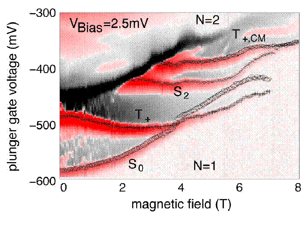
Figure 9: (Color online) Differentiated current $\rmd I/\rmd V_{\mathrm{pg}}$ at $V_{\mathrm{bias}}=2.5$ mV (the subscript ${\rm pg}$ denotes the plunger gate). Gray striped regions (red online) marked by symbols correspond to positive (peaks) $dI/dV_{\mathrm{pg}}$. The dark black region (also black online) corresponds to negative $dI/dV_{\mathrm{pg}}$. Electron numbers $N$ are indicated. Transitions between the one-electron ground state and the 2$e$ spin-singlet ground (excited for $B>3.8$ T) state ($S_{0}$), spin-triplet excited (ground for $B>3.8$ T) state ($T_{+}$), spin-singlet excited state ($S_{2}$), and spin-triplet plus center-of-mass excited state ($T_{+,{\rm CM}}$) are labeled.

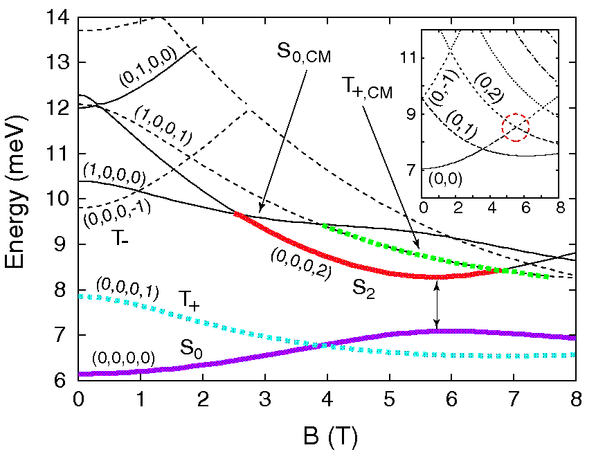
Figure 10: (Color online) Calculated exact-diagonalization energy spectrum in a magnetic field, referenced to $2\hbar\sqrt{\omega_{0}^{2}+\omega_{c}^{2}/4}$, of a 2$e$ dot with anisotropic harmonic confinement (for the dot parameters, see text). We have adopted the notation $(N_{x},N_{y},n,m)$, where $(N_{x},N_{y})$ refer to the CM motion along the $x$ and $y$ axes and $(n,m)$ refer to the number of radial nodes and angular momentum of the relative motion in the corresponding circular dot. Inset: The EXD spectrum of the corresponding circular dot. Only the $(n,m)$ indices are shown, since $N_{x}=N_{y}=0$ for all the plotted curves. Solid lines denote singlets. Dashed lines denote triplets.

As shown in Ref. [41], the experimental findings can be quantitatively interpreted by comparing to the results of the EXD calculations for two electrons in an anisotropic harmonic confinement potential with the parameters listed above. All the states observed in the measured spectra (as a function of the magnetic field) can be unambiguously identified [41] with calculated ground-state and excited states of the two-electron Hamiltonian (compare figure 9 and figure 10).

Moreover, the calculated magnetic-field-dependent energy splitting, $J_{\rm{EXD}}(B)=E^{t}_{\rm{EXD}}(B)-E^{s}_{\rm{EXD}}(B)$, between the two lowest singlet ($S_{0}$) and triplet ($T_{+}$) states is found to be in remarkable agreement with the experiment [see figure 11].

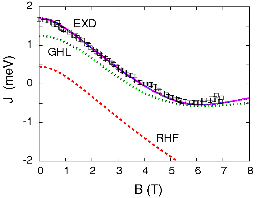
Figure 11: (Color online) Comparison between the lowest-triplet/lowest-singlet energy splitting [$J(B)$] calculated with different methods and the experimental results (open squares). Solid line (online magenta): EXD. Dotted line (online green): GHL. Dashed line (online red): RHF. For the parameters used in the calculation to model the anisotropic QD, see text.

A deeper understanding of the structure of the many-body wave function can be acquired by comparing the measured $J(B)$ with that calculated within the GHL and RHF approximations. To facilitate the comparisons, the calculated $J_{\rm{GHL}}(B)$ and $J_{\rm{RHF}}(B)$ curves are plotted also in figure 11, along with the exact-diagonalization result and the measurements. Both the RHF and GHL schemes are appealing intuitively, because they minimize the total energy using single-particle orbitals. It is evident, however, from figure 11 that the RHF method, which assumes that both electrons occupy a common single-particle orbital, is not able to reproduce the experimental findings. On the contrary, the generalized Heitler-London approach, which allows the two electrons to occupy two spatially separated orbitals, appears to be a good approximation. Plotting the two GHL orbitals [see figure 12] for the singlet state clearly demonstrates that the two electrons do not occupy the same orbital, but rather fill states that are significantly spatially separated.

Figure 12: (Color online) Single-particle UHF orbitals (modulus square) that are used in the construction of the GHL wave function in (5.3). Arrows indicate up and down spins. For the parameters used in the calculation to model the anisotropic QD, see text. Lengths in nm and orbital densities in 10^-3 nm^-2.

The UHF orbitals from which the GHL singlet state is constructed [see (5.3)] are displayed on figure 12 for both the $B=0$ and $B=3.8$ T cases. The spatial shrinking of these orbitals at the higher $B$-value illustrates the “dissociation” of the electron dimer with increasing magnetic field. The asymptotic convergence (beyond the ST point) of the energies of the singlet and triplet states, [i.e., $J(B)\rightarrow 0$ as $B\rightarrow\infty$] is a reflection of the dissociation of the 2$e$ molecule, since the ground-state energy of two fully spatially separated electrons (zero overlap) does not depend on the total spin. We stress again that the RHF, which corresponds to the more familiar physical picture of a QD-Helium atom, fails to describe this dissociation, because $J_{\rm{RHF}}(B)$ diverges as the value of the magnetic field increases.

In contrast to the RHF, the GHL wave function is able to capture the importance of correlation effects. Further insight into the inportance of correlations in our QD device can be gained through inspection [41] of the conditional probability distributions [see (1.1)] associated with the EXD solutions; see an illustration in figure 13. Indeed, already at zero magnetic field, the calculated CPDs provide further support of the physical picture of two localized electrons forming a state resembling an H₂-type [23, 46, 41] Wigner molecule [20, 188].

Figure 13: (Color online) CPDs extracted from the exact-diagonalization wave function for the singlet state for $B=0$ and $B=3.8$ T. The CPD expresses the conditional probability for finding the second electron at position ${\bf r}$ given that the first electron is located at ${\bf r}_{0}$ (denoted by a heavy solid dot). For the parameters used in the calculation to model the anisotropic QD, see text. Lengths in nm and CPDs in arbitrary units.

5.1.4 Degree of entanglement.

Further connections between the strong correlations found in our microscopic treatment and the theory of quantum computing [48] can be made through specification of the degree of entanglement between the two localized electrons in the molecular dimer. For two electrons, we can quantify the degree of entanglement by calculating a well-known measure of entanglement such as the von Neumann entropy [42, 200] for indistinguishable particles. To this effect, one needs to bring the EXD wave function into a diagonal form (the socalled “canonical form” [200, 201]), i.e.,

$$\Psi^{s,t}_{\rm{EXD}}({\bf r}_{1},{\bf r}_{2})=\sum_{k=1}^{M}z^{s,t}_{k}|\Phi(1;2k-1)\Phi(2;2k)\rangle,$$ (5.6)

with the $\Phi(i)$’s being appropriate spin orbitals resulting from a unitary transformation of the basis spin orbitals $\psi(j)$’s [see (5.5)]; only terms with $z_{k}\neq 0$ contribute. The upper bound $M$ can be smaller (but not larger) than $K$ (the dimension of the single-particle basis); $M$ is referred to as the Slater rank. One obtains the coefficients of the canonical expansion from the fact that the $|z_{k}|^{2}$ are eigenvalues of the hermitian matrix ${\cal A}^{\dagger}{\cal A}$ [${\cal A}$, see (5.5), is antisymmetric]. The von Neumann entropy is given by ${\cal S}=-\sum_{k=1}^{M}|z_{k}|^{2}\log_{2}(|z_{k}|^{2})$ with the normalization $\sum_{k=1}^{M}|z_{k}|^{2}=1$.

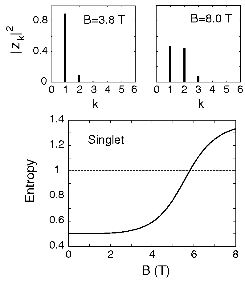
Figure 14: Von Neumann entropy for the lowest singlet EXD state of the elliptic dot as a function of the magnetic field $B$. On the top, we show histograms for the $|z_{k}|^{2}$ coefficients [see (5.6)] of the singlet state at $B=3.8$ T (left) and $B=8.0$ T (right) illustrating the dominance of two determinantal configurations (in agreement with the generalized Heitler-London picture). Note the small third coefficient $|z_{3}|^{2}=0.081$ for $B=8.0$ T. For the parameters used to model the experimental device, see text.

The EXD singlet has obviously a Slater rank $M>2$. The von Neumann entropy for the EXD singlet (${\cal S}^{s}_{\rm{EXD}}$) is displayed in figure 14. It is remarkable that ${\cal S}^{s}_{\rm{EXD}}$ increases with increasing $B$, but remains close to unity for large $B$, although the maximum allowed mathematical value is $\log_{2}(K)$ [for example, for $K=79$, $\log_{2}(79)=6.3$]. The saturation of the entropy for large $B$ to a value close to unity reflects the dominant (and roughly equal at large $B$) weight of two configurations in the canonical expansion [see (5.6)] of the exact-diagonalization wave function, which are related [42] to the two terms in the canonical expansion of the GHL singlet. This is illustrated by the histograms of the $|z_{k}^{s}|^{2}$ coefficients for $B=3.8$ T and $B=8.0$ T in figure 14 (top). Notice that the ratio $|z_{2}|^{2}/|z_{1}|^{2}$ reflects the extent of the overlap between the two GHL orbitals [42], with the ratio increasing for smaller overlaps (corresponding to a more complete dissociation of the Wigner molecule).

The above discussion illustrates that microscopic calculations that are shown to reproduce experimental spectra [41] can be used to extract valuable information that allows assessment of the suitability of a given device for quantum computations.

5.2 Two-electron circular dots at zero magnetic field

In section 2.2, we illustrated the formation of “rotating electron molecules” in the case of a two-electron circular QD, where one needs to consider restoration of the rotational symmetry as well, in addition to the restoration of the total spin. There, we focused on properties of the ground state ($L=0$).

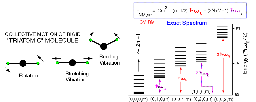
Figure 15: (Color online) The calculated spectrum of a two-electron circular parabolic quantum dot, with $R_{W}=200$. The quantum numbers are $(N,M,n,m)$ with $N$ corresponding to the number of radial nodes in the center of mass (CM) wavefunction, and $M$ is the CM azimuthal quantum number. The integers $n$ and $m$ are the corresponding quantum numbers for the electrons’ relative motion (RM) and the total energy is given by $E_{NM,nm}=E^{\rm CM}_{NM}+E^{\rm RM}(n,|m|)$. The spectrum may be summarized by the “spectral rule” given in the figure, with an effective rigid moment of inertia $C=0.037$ (corresponding to an angular momentum ${\cal L}=\hbar m$), the phonon for the stretching vibration $\hbar\omega_{s}=3.50$, and the phonon for the bending vibration coincides with that of the CM motion, i.e., $\hbar\omega_{b}=\hbar\omega_{0}=2$. The quantum numbers $(N_{0},M_{0},n_{0},m)$ specifying each rotational band are given at the bottom, with $m=0,1,2,\ldots$ (the levels $m=0$ and $m=1$ in each band may not be resolved on the scale of the figure). We note that the energy separation between levels in a given rotational band increases as $(2m+1)$ with increasing $m$, which is a behavior characteristic of a rigid rotor. All energies are in units of $\hbar\omega_{0}/2$, where $\omega_{0}$ is the parabolic confinement frequency.

In this section, we will further examine the excitation spectra of a two-electron QD by using the rather simple exact solution of this problem provided through separation of the center-of-mass and inter-electron relative-distance degrees of freedom [50]. The spectrum obtained for $R_{W}=200$ (figure 15), exhibits features that are characteristic of a collective rovibrational dynamics, akin to that of a natural “near-rigid” triatomic linear molecule with an infinitely heavy middle particle representing the center of mass of the dot. This spectrum transforms to that of a “floppy” molecule for smaller value of $R_{W}$ (i.e., for stronger confinements characterized by a larger value of $\omega_{0}$, and/or for weaker inter-electron repulsion), ultimately converging to the independent-particle picture associated with the circular central mean-field of the QD.

Further evidence for the formation of the electron molecule and the emergence of a rovibrational spectrum was found through examination [50] of the conditional probability distributions for various states $(N,M,n,m)$ (see the caption of figure 15 for the precise meaning of these quantum numbers labeling the spectra). As an example, we display in figure 16 the CPD for the bottom state ($m=0$) of the rotational band $(1,0,1,m)$ (not shown in figure 15); it reveals that this state corresponds to a vibrational motion of the electron molecule both along the interelectron axis (one excited stretching-mode phonon; see figure 15) and perpendicularly to this axis (two excited bending-mode phonons; see figure 15).

It is instructive to note here certain similarities between the formation of a “two-electron molecule” in man-made quantum dots, and the collective (rovibrational) features observed in the electronic spectrum of doubly-excited helium atoms [202, 203, 204].

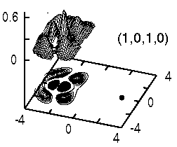
Figure 16: CPD of the excited multi-vibrational state (1,0,1,0) of a $2e$ circular parabolic QD with $R_{W}=200$ (see text for details). The solid dot portrays the position of the reference point ${\bf r}_{0}=(d_{0},0)$, where $d_{0}=2.6$ is half the interelectron distance at the ground state $(0,0,0,0)$. Distances are in units of $l_{0}\sqrt{2}$; the scale of the vertical axis is arbitrary.

5.3 Historical significance of the two-electron problem

In spite of being the simplest many-body system, the significance of the problem of two interacting electrons confined in an external potential cannot be overstated. Historically it played a central role in the development of the quantum theory of matter through the failure of the Bohr-type semiclassical models to account for the natural He atom. Most recently it has influenced the development of several fields like nonlinear physics, atomic physics, semiconductror quantum dots, and quantum computing.

It is instructive to make here a historical detour. Indeed, the failure of Bohr-type semiclassical models, based on the orbiting of spatially correlated (antipodal) electrons in conjunction with the Bohr-Sommerfeld quantization rule, to yield a reasonable estimate of the ground state of the He atom signaled a looming crisis in physics in the 1920’s, which Bohr himself, as well as others, had been keenly aware of, as summarized succintly by Sommerfeld: “All attempts made hitherto to solve the problem of the neutral helium atom have proved to be unsuccessful” [205]; see also the 10th chapter entitled “It was the Spring of hope, it was the Winter of despair” in the book by Pais [206], the review by Van Vleck [207] and the book by Born [208].

While, since, numerical solutions of the two-electron Schrödinger equation provided a quantitative resolution to the problem, the first successful semiclassical treatment of the three-body Coulomb system awaited till 1980 [209, 210].

Furthermore, based on rather general group-theoretical arguments arising from the observation of hierarchies with lower symmetry in the excited spectra, and motivated by ideas originating in nuclear-physics spectroscopy, it has been discovered in the late 1970’s and early 1980’s that electron correlations in doubly excited He lead to quantization of the spectrum much like in a linear triatomic molecule, $e$-He²⁺-$e$. This molecular picture, with near rigidity and separability, results in “infinite sequences of vibrational levels, on each of which is built an infinite sequence of rotational levels” [202, 211, 212].

The two previous section 5.1 and section 5.2 describing the formation and properties of a 2$e$ Wigner molecule in a single QD may be viewed as the culmination of this historical background. Interestingly, as in the aforementioned semiclassical treatments, the collinear configuration plays a special role in the molecule-like model, serving perhaps as “partial vindication” of the geometry considered originally by Niels Bohr.

6 Rotating electron molecules in two-dimensional quantum dots under a strong magnetic field: The case of the lowest Landau level ($\omega_{c}/2\omega_{0}\rightarrow\infty$)

6.1 REM analytic trial wave functions

In the last ten years, and in particular since 1999 (when it was explicitly demonstrated [20] that Wigner crystallization for small systems is related to symmetry breaking at the unrestricted Hartree-Fock mean-field level), the number of publications addressing the formation and properties of Wigner (or electron) molecules in 2D QDs and quantum dot molecules has grown steadily [20, 21, 23, 24, 27, 50, 101, 102, 128, 132, 167, 171, 175, 188, 189, 195, 213, 214, 215, 216, 217, 218, 219, 220, 221]. A consensus has been reached that rotating electron molecules are formed both in zero [21, 23, 24, 46, 50, 101, 167, 175, 188, 189, 195, 213, 214, 215, 216, 217, 218, 219] and high [26, 27, 46, 102, 128, 131, 132, 171, 220, 221] magnetic fields.

At $B=0$, in spite of considerable differences explored in this report (see next paragraph), formation of REMs in quantum dots is driven by the same physical factors as Wigner crystallization in infinite 2D media, i.e., when the strength of the interelectron repulsion relative to the zero-point kinetic energy ($R_{W}$) exceeds a certain critical value, electrons spontaneously crystallize around sites forming geometric molecular structures. At high magnetic fields, the formation of Wigner molecules may be thought of as involving a two-step crystallization process: (I) the localization of electrons results from the shrinkage of the orbitals due to the increasing strength of the magnetic field; (II) then, even a weak interelectron Coulomb repulsion is able to arrange the localized electrons according to geometric molecular structures (thus this process is independent of the value of $R_{W}$). It has been found [24, 26, 27, 128] that the molecular structures at high $B$ coincide with the equilibrium configurations at $B=0$ of $N$ classical point charges [112, 113, 114, 222].

Due to the small finite number, $N$, of electrons, however, there are two crucial differences between the REM and the bulk Wigner crystal. Namely, (I) the crystalline structure is that of the equilibrium 2D configuration of $N$ classical point charges, and thus consists of nested polygonal rings, in contrast to the well known hexagonal bulk crystal;

(II) in analogy with the case of 3D natural molecules, the Wigner molecules rotate as a whole (collective rotations); they behave, however, as highly floppy (non-rigid) rotors.

A most striking observation concerning the REMs is that their formation and properties have been established with the help of traditional ab initio many-body methods, i.e., exact diagonalization, [50, 128, 131, 167, 171, 213, 221] quantum Monte Carlo [78, 188, 195, 196, 216], and the systematic controlled hierarchy [20, 22, 23, 24, 25, 27, 102, 217] of approximations involving the UHF and subsequent post-Hartree-Fock methods. This contrasts with the case of the Jastrow/Laughlin [55] and composite-fermion [56, 57] wave functions, which were constructed through “intuition-based guesswork.”

In spite of its appearance in the middle nineties and its firm foundation in many-body theory, however, the REM picture had not, until recently, successfully competed with the CF/JL picture; indeed many research papers [181, 223, 224, 225, 226, 227, 228] and books [133] describe the physics of quantum dots in high magnetic fields following exclusively notions based on CF/JL functions, as expounded in 1983 (see Ref. [55]) and developed in detail in 1995 in Ref. [229] and Ref. [174]. One of the main obstacles for more frequent use of the REM picture had been the lack of analytic correlated wave functions associated with this picture. This situation, however, changed with the recent explicit derivation of such REM wave functions [24].

The approach used in Ref. [24] for constructing the analytic REM functions in high $B$ consists of two-steps: First the breaking of the rotational symmetry at the level of the single-determinantal unrestricted Hartree-Fock approximation yields states representing electron molecules. Subsequently the rotation of the electron molecule is described through restoration of the circular symmetry via post Hartree-Fock methods, and in particular Projection Techniques [18]. The restoration of symmetry goes beyond the single determinantal mean-field description and yields multi-determinantal wave functions.

In the zero and low-field cases, the broken symmetry UHF orbitals need to be determined numerically, and, in addition, the restoration of the total-spin symmetry needs to be considered for unpolarized and partially polarized cases. The formalism and mathematical details of this procedure at $B=0$ have been elaborated in previous sections.

In the case of high magnetic fields, the spins of the electrons are fully polarized. Furthermore, one can specifically consider the limit when the confining potential can be neglected compared to the confinement induced by the magnetic field, so that the Hilbert space is restricted to the lowest Landau level. Then, assuming a symmetric gauge, the UHF orbitals can be represented [24, 230] by displaced Gaussian analytic functions, centered at different positions $Z_{j}\equiv X_{j}+\rmi Y_{j}$ according to the equilibrium configuration of $N$ classical point charges [112, 113, 114, 222] arranged at the vertices of nested regular polygons (each Gaussian representing a localized electron). Such displaced Gaussians in the lowest Landau level are written as

$$u(z,Z_{j})=(1/\sqrt{\pi})\exp[-|z-Z_{j}|^{2}/2]\exp[-\rmi(xY_{j}-yX_{j})],$$ (6.1)

where the phase factor is due to the gauge invariance. $z\equiv x+\rmi y$, and all lengths are in dimensionless units of ${l_{B}}\sqrt{2}$ with the magnetic length being $l_{B}=\sqrt{\hbar c/eB}$. Note that expression (6.1) is a special case of the more general expression (2.24) for a displaced Gaussian which corresponds to situations with smaller magnetic fields when the restriction to the lowest Landau level breaks down. The notation $z\equiv x+\rmi y$ is associated with positive angular momenta for the single-particle states in the lowest Landau level. Ref. [24] used $z\equiv x-\rmi y$ and negative single-particle angular momenta in the lowest Landau level. The final expressions for the trial wave functions do not depend on these choices.

Table 1: Comparison of yrast-band energies obtained from REM and EXD calculations for $N=6$ electrons in the lowest Landau level, that is in the limit $B\rightarrow\infty$. In this limit the external confinement can be neglected and only the interaction energy contributes to the yrast-band energies. Energies in units of $e^{2}/(\kappa l_{B})$. For the REM results, the (1,5) polygonal-ring arrangement was considered. The values of the fractional filling may be obtained for each $L$ as $\nu=N(N-1)/(2L)$.

• $L$	REM	EXD	Error (%)	$L$	REM	EXD	Error (%)
  70	2.3019	2.2824	0.85	140	1.6059	1.6006	0.33
  75	2.2207	2.2018	0.85	145	1.5773	1.5724	0.31
  80	2.1455	2.1304	0.71	150	1.5502	1.5455	0.30
  85	2.0785	2.0651	0.65	155	1.5244	1.5200	0.29
  90	2.0174	2.0054	0.60	160	1.4999	1.4957	0.28
  95	1.9614	1.9506	0.55	165	1.4765	1.4726	0.27
  100	1.9098	1.9001	0.51	170	1.4542	1.4505	0.26
  105	1.8622	1.8533	0.48	175	1.4329	1.4293	0.25
  110	1.8179	1.8098	0.45	180	1.4125	1.4091	0.24
  115	1.7767	1.7692	0.42	185	1.3929	1.3897	0.23
  120	1.7382	1.7312	0.40	190	1.3741	1.3710	0.23
  125	1.7020	1.6956	0.38	195	1.3561	1.3531	0.22
  130	1.6681	1.6621	0.36	200	1.3388	1.3359	0.21
  135	1.6361	1.6305	0.34

Ref. [24] used these analytic orbitals to first construct the broken symmetry UHF determinant, $\Psi^{\rm{UHF}}_{N}$, and then proceeded to derive analytic expressions for the many-body REM wave functions by applying onto $\Psi^{\rm{UHF}}_{N}$ an appropriate projection operator ${\cal P}_{L}$ (see section 2.2.1) that restores the circular symmetry and generates correlated wave functions with good total angular momentum $L$. These REM wave functions can be easily written down [24] in second-quantized form for any classical polygonal ring arrangement $(n_{1},n_{2},\ldots,n_{r})$ by following certain simple rules for determining the coefficients of the determinants $D(l_{1},l_{2},\ldots,l_{N})\equiv{\rm{det}}[z_{1}^{l_{1}},z_{2}^{l_{2}},\cdot\cdot\cdot,z_{N}^{l_{N}}]$, where the $l_{j}$’s denote the angular momenta of the individual electrons.

The REM functions associated with the $(0,N)$ and $(1,N-1)$ ring arrangements, respectively [here $(0,N)$ denotes a regular polygon with $N$ vertices, such as an equilateral triangle or a regular hexagon, and $(1,N-1)$ is a regular polygon with $N-1$ vertices and one occupied site in its center], are given by

$$\Phi_{L}^{(0,N)}(z_{1},z_{2},\ldots,z_{N}) =\sum^{l_{1}+\cdot\cdot\cdot+l_{N}=L}_{0\leq l_{1}<l_{2}<\cdot\cdot\cdot<l_{N}}\left(\prod_{i=1}^{N}l_{i}!\right)^{-1}\left(\prod_{1\leq i<j\leq N}\sin\left[\frac{\pi}{N}(l_{i}-l_{j})\right]\right)$$ (6.2)

$$\times\;D(l_{1},l_{2},\ldots,l_{N})\exp(-\sum_{i=1}^{N}z_{i}z_{i}^{*}/2),$$

with

$$L=L_{0}+Nm,\;\;m=0,1,2,3,\ldots,$$ (6.3)

and

$$\Phi_{L}^{(1,N-1)}(z_{1},z_{2},\ldots,z_{N}) =\sum^{l_{2}+\cdot\cdot\cdot+l_{N}=L}_{1\leq l_{2}<l_{3}<\cdot\cdot\cdot<l_{N}}\left(\prod_{i=2}^{N}l_{i}!\right)^{-1}\left(\prod_{2\leq i<j\leq N}\sin\left[\frac{\pi}{N-1}(l_{i}-l_{j})\right]\right)$$ (6.4)

$$\times\;D(0,l_{2},\ldots,l_{N})\exp(-\sum_{i=1}^{N}z_{i}z_{i}^{*}/2),$$

with

$$L=L_{0}+(N-1)m,\;\;m=0,1,2,3,\ldots,$$ (6.5)

where $L_{0}=N(N-1)/2$ is the minimum allowed total angular momentum for $N$ (fully spin polarized) electrons in high magnetic fields.

Notice that the REM wave functions [Equation (6.2) and Equation (6.4)] vanish identically for values of the total angular momenta outside the specific values given by the sequences (6.3) and (6.5), respectively; these sequences are termed as magic angular momentum sequences.

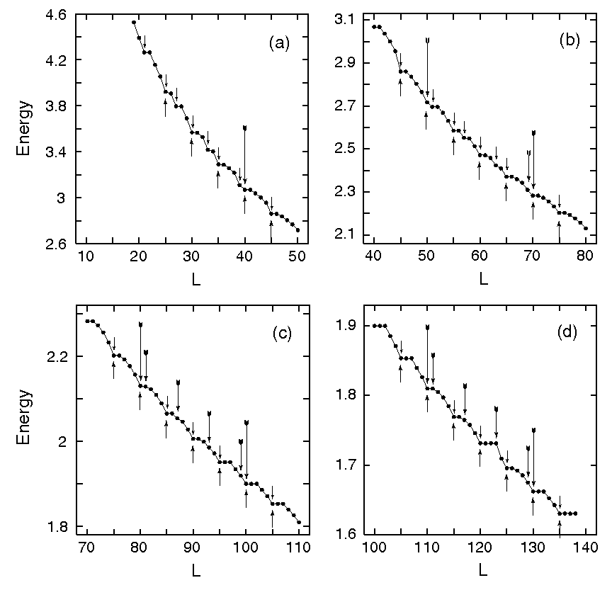
Figure 17: Total interaction energy from exact-diagonalization calculations as a function of the total angular momentum $(19\leq L\leq 140)$ for $N=6$ electrons in the lowest Landau level. The upwards pointing arrows indicate the magic angular momenta corresponding to the classically most stable (1,5) polygonal ring arrangement of the Wigner molecule. The short downwards pointing arrows indicate successful predictions of the composite-fermion model. The medium-size downwards pointing arrows indicate predictions of the composite-fermion model that fail to materialize as magic angular momenta. The long downward arrows indicate EXD magic angular momenta not predicted by the composite-fermion model. Energies in units of $e^{2}/\kappa l_{B}$, where $\kappa$ is the dielectric constant.

We remark that, while the original REM analytic wave function was derived in the context of a high magnetic field (that is in the fractional quantum Hall effect regime), it is valid for any circumstance where the spectrum consists of a degenerate manifold of LLL-like states (even with no magnetic field present). Indeed a wave function having the form of the REM wave function discussed by us above has been employed recently for graphene quantum dots with a zig-zag boundary condition and in the absence of a magnetic field [231].

In the remaining of this section, we continue discussing the properties of analytic REM wave functions associated with fully spin polarized electrons. However, we mention here that, following the methodology of Ref. [24] for fully spin polarized REMs. Dai et al[232] and Shi et al[233] have most recently presented analytic trial wave functions for rotating electron molecules with partial spin polarizations.

6.2 Yrast rotational band in the lowest Landau level

As an accuracy test, we compare in table 1 REM and exact-diagonalization results for the interaction energies of the yrast band associated with the magic angular momenta $L_{m}$ [see (2.26)] of $N=6$ electrons in the lowest Landau level. An yrast state is defined as the lowest-energy state for a given angular momentum $L$. As a result, the yrast band represents excitations with purely rotational motion; no other excitations, like center-of-mass or vibrational modes, are present.

As seen from table 1, the REM wave functions offer an excellent approximation to the EXD ones, since the relative error of the REM energies is smaller than 0.3%, and it decreases steadily for larger $L$ values. Of course, a small difference in the energies between approximate and exact-diagonalization results is only one of several tests for deciding whether a given trial wave function is a good approximation. As will be discussed below, comparison of conditional probability distrubutions is an equally (if not more) important test.

6.3 Inconsistencies of the composite-fermion view for semiconductor quantum dots.

Before the development of the REM approach, electrons in the lowest Landau level in two-dimensional quantum dots were thought as being well approximated by composite fermion trial wave functions. However, results obtained with the REM and exact-diagonalization calculations led researchers to examine inconsistencies and discrepancies of the CF approach in the context of quantum dots. This section focuses on these issues.

For $N=6$, figure 17 displays (in four frames) the total interaction energy from exact-diagonalization as a function of the total angular momentum $L$ in the range $19\leq L\leq 140$. [The total kinetic energy in the Hamiltonian (4.1), being a constant, can be disregarded.] One can immediately observe the appearance of downward cusps, implying states of enhanced stability, at certain magic angular momenta.

For the CF theory, the magic angular momenta can be determined by

$$L=L^{*}+mN(N-1)=L^{*}+2mL_{0}.$$ (6.6)

Namely, for $N=6$, if one knows the non-interacting $L^{*}$’s, the CF magic $L$’s in any filling-factor interval $1/(2m-1)\geq\nu\geq 1/(2m+1)$ [corresponding to the angular-momentum interval $15(2m-1)\leq L\leq 15(2m+1)]$, $m=1,2,3,4,\ldots$, can be found by adding $2mL_{0}=30m$ units of angular momentum to each of the $L^{*}$’s. To obtain the non-interacting $L^{*}$’s, one needs first to construct [26, 131, 229] the compact Slater determinants. Let $N_{n}$ denote the number of electrons in the $n$th Landau level with $\sum_{n=0}^{t}N_{n}=N$; $t$ is the index of the highest occupied Landau level and all the lower Landau levels with $n\leq t$ are assumed to be occupied. The compact determinants are defined as those in which the $N_{n}$ electrons occupy contiguously the single-particle orbitals (of each $n$th Landau level) having the lowest angular momenta $l=-n,-n+1,\ldots,-n+N_{n}-1$. The compact Slater determinants are usually denoted as $[N_{0},N_{1},\ldots,N_{t}]$; see Refs. [25, 229] for details.

The compact determinants and the corresponding non-interacting $L^{*}$’s for $n=6$ are listed in Table 2.

Table 2: Compact Slater determinants and associated angular momenta $L^{*}$ for $N=6$ electrons according to the CF presciption. Both $L^{*}=-3$ and $L^{*}=3$ are associated with two compact states each, the one with lowest energy being the preferred one.

• Compact state	$L^{*}$
  $[$1,1,1,1,1,1$]$	$-$15
  $[$2,1,1,1,1$]$	$-$9
  $[$2,2,1,1$]$	$-$5
  $[$3,1,1,1$]$	$-$3
  $[$2,2,2$]$	$-$3
  $[$3,2,1$]$	0
  $[$4,1,1$]$	3
  $[$3,3$]$	3
  $[$4,2$]$	5
  $[$5,1$]$	9
  $[$6$]$	15

There are nine different values of $L^{*}$’s, and thus the CF theory for $N=6$ predicts that there are always nine magic numbers in any interval $15(2m-1)\leq L\leq 15(2m+1)$ between two consecutive angular momenta of Jastrow/Laughlin states, $15(2m-1)$ and $15(2m+1)$, $m=1,2,3,\ldots$ (henceforth we will denote this interval as ${\cal I}_{m}$). For example, using Table 2 and (6.6), the CF magic numbers in the interval $15\leq L\leq 45$ ($m=1$) are found to be the following nine

$$15,\;21,\;25,\;27,\;30,\;33,\;35,\;39,\;45.$$ (6.7)

On the other hand, in the interval $105\leq L\leq 135$ ($m=4$), the CF theory predicts the following set of nine magic numbers,

$$105,\;111,\;115,\;117,\;120,\;123,\;125,\;129,\;135.$$ (6.8)

An inspection of the total-energy-vs-$L$ plots in figure 17 reveals that the CF prediction misses the actual magic angular momenta specified by the exact-diagonalization calculations as those associated with the downward cusps. It is apparent that the number of downward cusps in any interval ${\cal I}_{m}$ is always different from 9. Indeed, there are 10 cusps in ${\cal I}_{1}$ [including that at $L=15$, not shown in figure 17(a)], 10 in ${\cal I}_{2}$ [see figure 17(b)], 7 in ${\cal I}_{3}$ [see figure 17(c)], and 7 in ${\cal I}_{4}$ [see figure 17(d)]. In detail, the CF theory fails in the following two aspects: (I) There are exact magic numbers that are consistently missing from the CF prediction in every interval; with the exception of the lowest $L=20$, these exact magic numbers (marked by a long downward arrow in the figures) are given by $L=10(3m-1)$ and $L=10(3m+1)$, $m=1,2,3,4,\ldots$; (II) There are CF magic numbers that do not correspond to downward cusps in the EXD calculations (marked by medium-size downward arrows in the figures). This happens because cusps associated with $L$’s whose difference from $L_{0}$ is divisible by 6 (but not simultaneously by 5) progressively weaken and completely disappear in the intervals ${\cal I}_{m}$ with $m\geq 3$; only cusps with the difference $L-L_{0}$ divisible by 5 survive. On the other hand, the CF model predicts the appearance of four magic numbers with $L-L_{0}$ divisible solely by 6 in every interval ${\cal I}_{m}$, at $L=30m\mp 9$ and $30m\mp 3$, $m=1,2,3,\ldots$ The overall extent of the inadequacy of the CF model can be appreciated better by the fact that there are six false predictions (long and medium-size downward arrows) in every interval ${\cal I}_{m}$ with $m\geq 3$, compared to only five correct ones [small downward arrows, see figure 17(c) and figure 17(d)].

In contrast to the CF model, the magic angular momenta in the REM theory are associated with the polygonal ring configurations of $N$ classical point charges. This is due to the fact that the enhanced stability of the downward cusps results from the coherent collective rotation of the regular-polygon REM structures. Due to symmetry requirements, such collective rotation can take place only at magic-angular-momenta values. The in-between angular momenta require the excitation of additional degrees of freedom (like the center of mass and/or vibrational modes), which raises the total energy with respect to the values associated with the magic angular momenta.

For $N=6$, the ring configuration of lowest energy is the (1,5), while there exists a (0,6) isomer [114, 222] with higher energy. As a result, our exact-diagonalization calculations [26] (as well as earlier ones [131, 132, 171] for lower angular momenta $L\leq 70$) have found that there exist two sequences of magic angular momenta, a primary one $(S_{p})$ with $L=15+5m$ [see Equation (6.5)], associated with the most stable (1,5) classical molecular configuration, and a secondary one $(S_{s})$ with $L=15+6m$ [see Equation (6.3)], associated with the metastable $(0,6)$ ring arrangement. Furthermore, our calculations (see also Refs. [132, 171]) show that the secondary sequence $S_{s}$ contributes only in a narrow range of the lowest angular momenta; in the region of higher angular momenta, the primary sequence $S_{p}$ is the only one that survives and the magic numbers exhibit a period of five units of angular momentum. It is interesting to note that the initial competition between the primary and secondary sequences, and the subsequent prevalence of the primary one, has been seen in other sizes as well [171] i.e., $N=5,7,8$. Furthermore, this competition is reflected in the field-induced molecular phase transitions associated with broken symmetry UHF solutions in a parabolic QD. Indeed, Ref. [53] demonstrated recently that, as a function of increasing $B$, the UHF solutions for $N=6$ first depict the transformation of the maximum density droplet [126] (see definition in section 2.2.1) into the (0,6) molecular configuration; then (at higher $B$) the (1,5) configuration replaces the (0,6) structure as the one having the lower HF energy.

The extensive comparisons in this section lead to the conclusion that the composite-fermion model does not explain the systematic trends exhibited by the magic angular momenta in 2D quantum dots in high magnetic fields. These trends, however, were shown to be a natural consequence of the formation of REMs and their metastable isomers.

These results motivated a reexamination of the original composite-fermion approach (the mean-field CF) and led to a reassessment of the significance of the residual interaction, neglected in the mean-field CF theory. Initially, it has been reported that some CF functions away from the main fractions [e.g., for $N=19$ and $L=1845$ and $N=19$ and $L=3555$] may reproduce the aforementioned crystalline patterns [234].

Subsequently, Jain and coworkers have found that inclusion of the residual interaction is absolutely necessary to account for the full range of inconsistencies of the mean-field CF theory [176]. However, this latter development was achieved with the trade off of abandoning the fundamental nature of the composite fermion as an elementary, independent and weakly interacting quasi-particle. Indeed, the revised [176] CF picture amounts to an exact diagonalization method which uses a correlated basis set (made out of CF wave functions).

Another attempt to update the CF theory in order to account for crystallization consists of combining the REM analytic wave function $\Phi^{\rm REM}_{L}(z_{1},z_{2},\ldots,z_{N})$ (see section 6.1) with Jastrow prefactors [235], namely one uses a variational wave function of the form

$$\Psi^{{2p,}{\rm CFC}}_{L}=\prod_{i<j}(z_{i}-z_{j})^{2p}\Phi^{\rm REM}_{L^{*}},$$ (6.9)

with $L=L^{*}+pN(N-1)$ and $p$ serves as an additional variational parameter. Obviously, the crystalline patterns in such an approach originate from the REM wave function and the Jastrow prefactors simply increase the variational freedom, leading to a numerical improvement. Although this approach is a straightforward variational improvement of the analytic REM method [24], it is being referred to [233, 235] as a composite-fermion crystal (CFC).

More direct variational improvements of the analytic REM wave functions can be devised in the spirit of the variation-after-projection method. For example, one can use angular-momentum conserving variational parameters in front of the sine coefficients in the REM expansion [231].

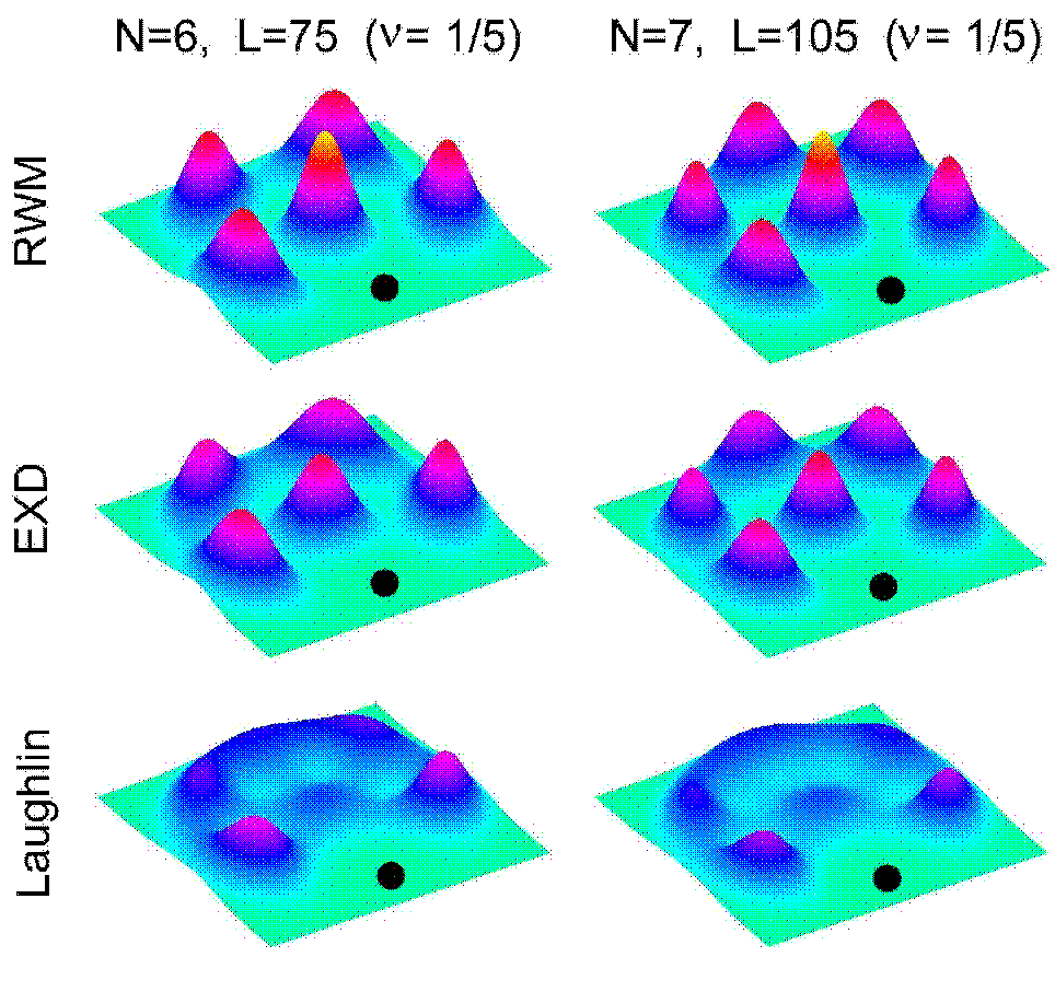
Figure 18: (Color online) Conditional probability distributions at high $B$ for $N=6$ electrons and $L=75$ ($\nu=1/5$, left column) and for $N=7$ electrons and $L=105$ (again $\nu=1/5$, right column). Top row: REM case. Middle row: The case of exact diagonalization. Bottom row: The Jastrow/Laughlin case. The exact diagonalization and REM wave functions have a pronouned crystalline character, corresponding to the (1,5) polygonal configuration of the REM for $N=6$, and to the (1,6) polygonal configuration for $N=7$. In contrast, the Jastrow/Laughlin wave functions exhibit a characteristic liquid profile that depends smoothly on the number $N$ of electrons. The observation point (identified by a solid dot) is located at $r_{0}=5.431l_{B}$ for $N=6$ and $L=75$ and $r_{0}=5.883l_{B}$ for $N=7$ and $L=105$. The EXD Coulomb interaction energies (lowest Landau level) are 2.2018 and 2.9144 $e^{2}/\kappa l_{B}$ for $N=6,L=75$ and $N=7,L=105$, respectively. The errors relative to the corresponding exact-diagonalization energies and the overlaps of the trial functions with the EXD ones are: (I) For $N=6,L=75$, REM: 0.85%, 0.817; JL: 0.32%, 0.837. (II) For $N=7,L=105$, REM: 0.59%, 0.842; JL: 0.55%, 0.754.

Figure 19: (Color online) CPDs at high $B$ for $N=7$ and $L=63$ ($\nu=1/3$). Top: REM case; Middle: EXD case; Bottom: JL case. Unlike the JL CPD (which is liquid), the CPDs for the exact-diagonalization and REM wave functions exhibit a well developed crystalline character [corresponding to the (1,6) polygonal configuration of the REM for $N=7$ electrons]. The observation point (identified by a solid dot) is located at $r_{0}=4.568l_{B}$.

6.4 REM versus Laughlin wave functions: Conditional probability distributions and multiplicity of zeroes

Recent extensive numerical calculations [24, 52] have revealed major disagreements between the intrinsic structure of the Jastrow/Laughlin trial wave functions [55] for the main fractions $\nu=1/(2m+1)$ and that of the exact-diagonalization and REM wave functions. Indeed, it was found that both EXD and REM wave functions exhibit crystalline correlations, while the Jastrow/Laughlin ones are liquid-like as originally described in Ref. [55].

To illustrate the differences between the intrinsic structure of the REM and EXD states in the lowest Landau level versus the familiar Jastrow/Laughlin ones, we display in figure 18 the CPDs for cusp states corresponding to a low filling factor $\nu=1/5$ and for two different sizes, i.e., for $N=6$ electrons ($L=75$, left column) and $N=7$ electrons ($L=105$, right column). In figure 18, the top row depicts the REM case; the EXD case is given by the middle row, while the CF case [which reduces to the JL wave functions for fractions $1/(2p+1)$] are given by the bottom row.

There are three principal conclusions that can be drawn from an inspection of figure 18 (and the many other cases studied in Ref. [26]).

(I) The character of the exact-diagonalization states is unmistakably crystalline with the EXD CPDs exhibiting a well developed molecular polygonal configuration [(1,5) for $N=6$ and (1,6) for $N=7$, with one electron at the center], in agreement with the explicitly crystalline REM case.

(II) For all the examined instances covering the low fractional fillings 1/9, 1/7, and 1/5, the Jastrow/Laughlin wave functions fail to capture the intrinsic crystallinity of the exact-diagonalization states. In contrast, they represent “liquid” states in agreement with an analysis that goes back to the original papers [55, 236] by Laughlin. In particular, Ref. [236] investigated the character of the JL states through the use of a pair correlation function [usually denoted by $g(R)$] that determines the probability of finding another electron at the absolute relative distance $R=|{\bf r}-{\bf r}_{0}|$ from the observation point ${\bf r}_{0}$. Our anisotropic CPD of Equation (1.1) is of course more general (and more difficult to calculate) than the $g(R)$ function of Ref. [236]. However, both our $P({\bf r},{\bf r}_{0})$ (for $N=6$ and $N=7$ electrons) and the $g(R)$ (for $N=1000$ electrons, and for $\nu=1/3$ and $\nu=1/5$) in Ref. [236] reveal a similar characteristic liquid-like and short-range-order behavior for the JL states, eloquently described in Ref. [236] (see p. 249 and p. 251). Indeed, we remark that only the first-neighbor electrons on the outer rings can be distinguished as separate localized electrons in our CPD plots of the JL functions [see figure 18].

(III) For a finite number of electrons, pronounced crystallinity of the exact-diagonalization states occurs already at the $\nu=1/5$ value (see figure 18). This finding is particularly interesting in light of expectations [234, 237] (based on comparisons [55, 236, 238] between the JL states and the static bulk Wigner crystal) that a liquid-to-crystal phase transition may take place only at lower fillings with $\nu\leq 1/7$.

Of interest also is the case of $\nu=1/3$. Indeed, for this fractional filling, the liquid JL function is expected to provide the best approximation, due to very high overlaps (better than 0.99) with the exact wave function [58, 59, 161]. In figure 19, we display the CPDs for $N=7$ and $L=63$ ($\nu=1/3$), and for the three cases of REM, EXD, and JL wave functions. Again, even in this most favorable case, the CPD of the JL function disagrees with the EXD one, which exhibits clearly a (1,6) crystalline configuration in agreement with the REM CPD.

Similar crystalline correlations at higher fractions were also found for quantum dots of larger sizes, e.g., $N=8$, and $N=9$ electrons. As illustrative examples for these additional sizes [see also the EXD CPD for $N=12$ electrons in figure 24 below (in section 7.3)], we displayed in figure 5 of Ref. [26] the CPDs for $N=8$ and $L=91$ ($1/5<\nu=4/13<1/3$) and for $N=9$ and $L=101$ ( $1/3<\nu=36/101<1$). Again, the CPDs (both for the REM and the EXD wave functions) exhibit a well developed crystalline character in accordance with the (1,7) and (2,7) polygonal configurations of the REM, appropriate for $N=8$ and $N=9$ electrons, respectively.

Another area of disagreement between REM and Laughlin wave functions concerns the properties of the zero points. In this respect, we recall that the Jastrow/Laughlin trial functions for $N$ electrons have the form

$$\Phi^{\rm JL}(z_{1},z_{2},\ldots,z_{N})=\left(\prod_{1\leq i<j\leq N}(z_{i}-z_{j})^{2m+1}\right)\exp(-\sum_{i=1}^{N}z_{i}z_{i}^{*}/2).$$ (6.10)

Due to the Jastrow factors $(z_{i}-z_{j})^{2m+1}$, it is apparent that the Laughlin expressions (6.10) (as a function of a given $z_{i}$) have $N-1$ zero points, each of order $2m+1$, which are bound to the positions of the remaining $N-1$ electrons. In contrast, as discussed in Ref. [24], the analytic REM wave functions do not have zeroes with order higher than unity. In particular, only $N-1$ of the REM zeroes are bound to the positions of the remaining electrons, while the rest of them are free. Recently, it has been shown through extensive numerical studies [239] that the properties of REM zeroes are in agreement with the behavior of the zeroes in exact-diagonalization wave functions; this is another indication of the superiority of the REM picture compared to the Laughlin theory.

Before exiting this discussion, we remark about discrepancies of the Laughlin quasihole theory in the context of quantum dots. In particular, we recall that the Laughlin quasihole, with $N$ additional units of angular momentum, has been conjectured to be the first excited state. However, LLL exact-diagonalization calculations for $N$ electrons in a quantum dot have revealed that this is not the case. Instead, the first excited state corresponds to an increment in the total angular momentum which varies as the number of electrons localized on one of the rings of the rotating electron molecule, usually the outermost one; see figure 26 in section 7.4 below.

7 Rotating electron molecules in two-dimensional quantum dots under a strong, but finite external magnetic field ($\omega_{c}/2\omega_{0}>1$)

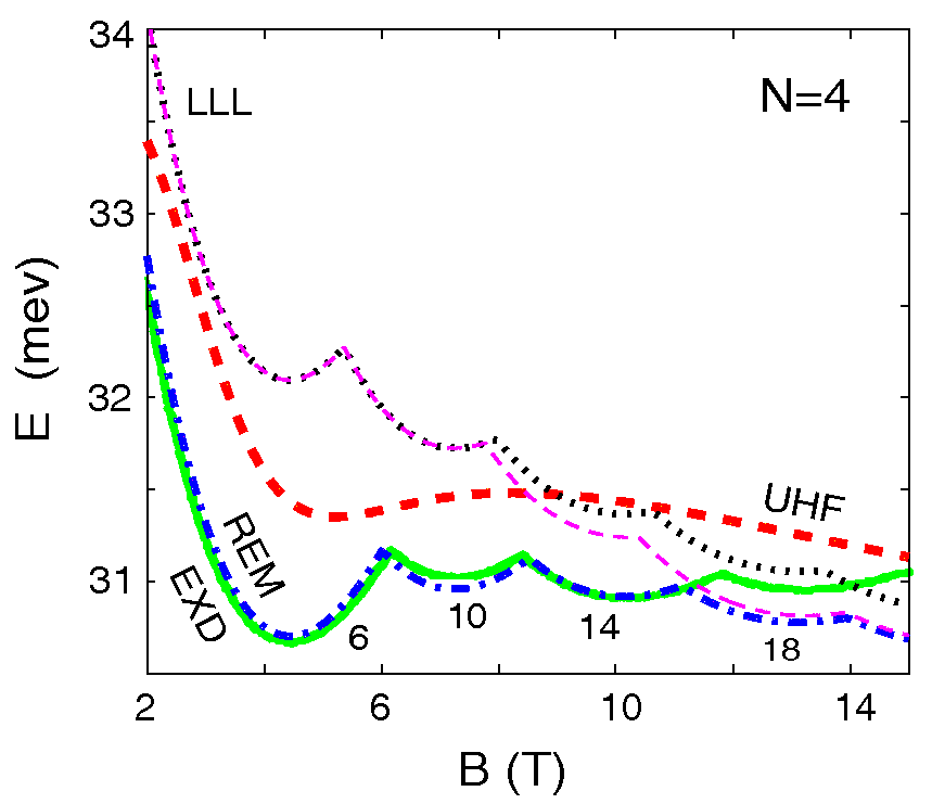
Figure 20: (Color online) Two-step-method versus exact-diagonalization calculations: Ground-state energies for $N=4$ electrons (referenced to $4\hbar\tilde{\omega}$) as a function of the magnetic field $B$. Thick dashed line (red): broken-symmetry UHF (static electron molecule). Solid line (green): EXD (from Ref. [171]). Thick dashed-dotted line (blue): REM. Thin dashed line (violet, marked LLL): the commonly used approximate energies $\tilde{E}^{\rm{EXD}}_{\rm{LLL}}(B)$ (see text for details). Thin dotted line (black): $\tilde{E}^{\rm{REM}}_{\rm{LLL}}(B)$ (see text). For $B<8$ T, the $\tilde{E}^{\rm{EXD}}_{\rm{LLL}}(B)$ and $\tilde{E}^{\rm{REM}}_{\rm{LLL}}(B)$ curves coincide; we have checked that these curves approach each other also at larger values of $B$, outside the plotted range. Numbers near the bottom curves denote the value of magic angular momenta [$L_{m}$, see (2.26)] of the ground state. Corresponding fractional filling factors are specified by $\nu=N(N-1)/(2L_{m})$. Parameters used: confinement $\hbar\omega_{0}=3.60$ meV, dielectric constant $\kappa=13.1$, effective mass $m^{*}=0.067m_{e}$.

7.1 Ground-state energies in medium and high magnetic field

The general form (2.24) for the displaced Gaussian orbitals [in conjunction with the projected REM wave function (2.25)] enables us to calculate REM ground-state energies for moderately-high $B$, when corrections arising from higher Landau levels must be taken into consideration. Unlike the lowest-Landau-level case, where the azimuthal integration can be carried out analytically, the energies (2.28) (and corresponding CPDs) associated with the general REM wave function (2.25) require numerical integration over the azimuthal angles $\gamma_{q}$.

Before proceeding with the presentation of results for $N>10$, we demonstrate the accuracy of the two-step method embodied in Equation (2.25) through comparisons with existing exact-diagonalization results for smaller sizes. In figure 20, our REM calculations for the ground-state energies as a function of $B$ are compared to EXD calculations [171] for $N=4$ electrons in an external parabolic confinement. The thick dotted line (red) represents the broken-symmetry UHF approximation (first step of our method), which naturally is a smooth curve lying above the EXD one [solid line (green)]. The results obtained after restoration of symmetry [dashed-dotted line (blue); marked as REM] agree very well with the EXD one in the whole range 2 T$<B<$ 15 T. We recall here that, for the parameters of the quantum dot, the electrons form in the intrinsic frame of reference a square about the origin of the dot, i.e., a (0,4) configuration, with the zero indicating that no electron is located at the center. According to (2.26), $L_{0}=6$, and the magic angular momenta are given by $L_{m}=6+4k$, $k=0$, 1, 2, $\ldots$ Note that the REM energies are slightly lower than the EXD ones in several subranges. According to the Rayleigh-Ritz variational theorem, this indicates that the hyperspherical-harmonics calculation (equivalent to an exact-diagonalization approach) of [171] did not converge fully in these subranges.

To further evaluate the accuracy of the two-step method, we also display in figure 20 [thin dashed line (violet)] ground-state energies $\tilde{E}^{\rm{EXD}}_{\rm LLL}(B)$ calculated with the commonly used approximate LLL Hamiltonian [128, 229, 237, 240]

$$\tilde{\cal H}_{\rm LLL}=N\hbar\tilde{\omega}+\hbar(\tilde{\omega}-\frac{\omega_{c}}{2})L+\sum_{j>i=1}^{N}\frac{e^{2}}{\kappa r_{ij}},$$ (7.1)

where $\tilde{\omega}=\sqrt{\omega_{0}^{2}+\omega_{c}^{2}/4}$. The LLL Hamiltonian $\tilde{\cal H}_{\rm LLL}$ reduces to the previously introduced Hamiltonian ${\cal H}_{\rm LLL}$ [see Equation (4.1)] in the limit $B\rightarrow\infty$. Both Hamiltonians restrict the many-body wave functions within the lowest Landau level, and they both accept the same set of eigenstates as solutions. Indeed the term $\hbar(\tilde{\omega}-\omega_{c}/2)L$ is proportional to the total angular momentum, and thus its presence influences only the eigenvalues, but not the composition of the eigenstates. $\tilde{\cal H}_{\rm LLL}$ corresponds to a situation where the external harmonic confinement is added to ${\cal H}_{\rm LLL}$ as a perturbation (see section II.B in Ref. [53]). As a result, (i) the degeneracy of the single-particle levels in the lowest Landau level is lifted and (ii) there is an eigenstate with minimum energy (the ground state) at each value of $B$ (expressed through the cyclotron frequency $\omega_{c}$). Naturally, the LLL levels used in the exact diagonalization of $\tilde{\cal H}_{\rm LLL}$ are given by expression (4.2), but with $\Lambda=\tilde{l}=\sqrt{\hbar/(m^{*}\tilde{\omega})}$.

We find that the energies $\tilde{E}^{\rm EXD}_{\rm LLL}(B)$ tend to substantially overestimate the REM (and EXD) energies for lower values of $B$ (e.g., by as much as 5.5% at $B\sim 4$ T). On the other hand, for higher values of $B$ ($>$ 12 T), the energies $\tilde{E}^{\rm{EXD}}_{\rm{LLL}}(B)$ tend to agree rather well with the REM ones. We stress that the results labelled simply as EXD correspond to exact diagonalizations without any restrictions on the Hilbert space, i.e., the full Darwin-Fock single-particle spectrum is considered at a given $B$.

A behavior similar to $\tilde{E}^{\rm EXD}_{\rm LLL}(B)$ is exhibited also by the $\tilde{E}^{\rm{REM}}_{\rm{LLL}}(B)$ ground-state energies [which are calculated using the Hamiltonian (7.1) and the LLL analytic REM wave functions in section 6.1 with lengths in units of $\sqrt{\hbar/(m^{*}\tilde{\omega})}$ instead of $l_{B}\sqrt{2}$; dotted line (black)]. A similar agreement between REM and EXD results, and a similar inaccurate behavior of the LLL approximate Hamiltonian (7.1) was found by us also for $N=3$ electrons in the range 2 T $<B<$ 16 T shown in figure 2 of Ref. [53] (the exact-diagonalization calculation in this figure was taken from Ref. [166]).

In all cases, the total energy of the REM is lower than that of the UHF Slater determinant (see, e.g., figure 20). Indeed, a theorem discussed in section 3 of Ref. [241], pertaining to the energies of projected wave functions, guarantees that this lowering of energy applies for all values of $N$ and $B$.

7.2 The case of $N=11$ electrons.

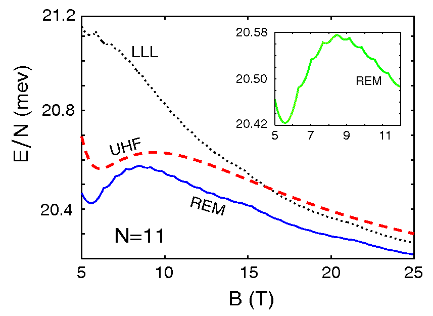
Figure 21: (Color online) Ground-state energies for $N=11$ electrons (per particle, referenced to $\hbar\tilde{\omega}$) as a function of the magnetic field $B$. Dashed line (red): UHF (static electron molecule). Solid line (blue): REM. Dotted line (black): Approximate energies $\tilde{E}^{\rm{REM}}_{\rm{LLL}}(B)$ (see text). Parameters used: confinement $\hbar\omega_{0}=3.60$ meV, dielectric constant $\kappa=13.1$, effective mass $m^{*}=0.067m_{e}$. The inset shows a magnification of the REM curve in the range 5 T $<B<$ 12 T.

Table 3: Ground-state magic angular momenta and their decomposition $\{k_{1},k_{2}\}$ for $N=11$ in the nagnetic-field range 5 T $\leq B\leq$ 25 T. The results correspond to the REM (see lower curve in figure 21). The parameters used are as in figure 21.

• $L_{m}$	$k_{1}$	$k_{2}$	$L_{m}$	$k_{1}$	$k_{2}$
  55	0	0	165	2	13
  63	0	1	173	2	14
  71	0	2	181	2	15
  79	0	3	189	2	16
  90	1	4	197	2	17
  98	1	5	205	2	18
  106	1	6	213	2	19
  114	1	7	224	3	20
  122	1	8	232	3	21
  130	1	9	240	3	22
  138	1	10	248	3	23
  146	1	11	256	3	24
  154	1	12

Figure 21 presents the case for the ground-state energies of a quantum dot with $N=11$ electrons, which have a nontrivial double-ring configuration $(n_{1},n_{2})$. The most stable [114] classical configuration is $(3,8)$, for which we have carried UHF (static electron molecule) and REM (projected) calculations in the magnetic field range 5 T $<B<$ 25 T. Figure 21 also displays the LLL ground-state energies $\tilde{E}^{\rm{REM}}_{\rm{LLL}}(B)$ [dotted curve (black)], which, as in previous cases, overestimate the ground-state energies for smaller $B$. The approximation $\tilde{E}^{\rm{REM}}_{\rm{LLL}}(B)$, however, can be used to calculate ground-state energies for higher values of $B$. In keeping with the findings for smaller sizes [51] [with $(0,N)$ or $(1,N-1)$ configurations], we found that both the UHF and the REM ground-state energies approach, as $B\rightarrow\infty$, the classical equilibrium energy of the (3,8) polygonal configuration [i.e., 19.94 meV; 4.865$E_{0}$ in the units of Ref. [114], $E_{0}\equiv(m^{*}\omega_{0}^{2}e^{4}/2\kappa^{2})^{1/3}$].

In analogy with smaller sizes (see, e.g., figure 20 and Ref. [53]), the REM ground-state energies in figure 21 exhibit oscillations as a function of $B$ (see in particular the inset). These oscillations are associated with magic angular momenta, specified by the number of electrons on each ring. For $N=11$ they are given by (2.26), i.e., $L_{m}=55+3k_{1}+8k_{2}$, with the $k_{q}$’s being nonnegative integers. As was the case with $N=9$ electrons [53], an analysis of the actual values taken by the set of indices $\{k_{1},k_{2}\}$ reveals several additional trends that further limit the allowed values of ground-state $L_{m}$’s. In particular, starting with the values $\{0,0\}$ at $B=5$ T ($L_{0}=55$), the indices $\{k_{1},k_{2}\}$ reach the values $\{3,24\}$ at $B=25$ T ($L_{m}=256$). As seen from table 3, the outer index $k_{2}$ changes faster than the inner index $k_{1}$. This behavior minimizes the total kinetic energy of the independently rotating rings; indeed, the kinetic energy of the inner ring (as a function of $k_{1}$) rises faster than that of the outer ring (as a function of $k_{2}$) due to smaller moment of inertia (smaller radius) of the inner ring [see (7.2)].

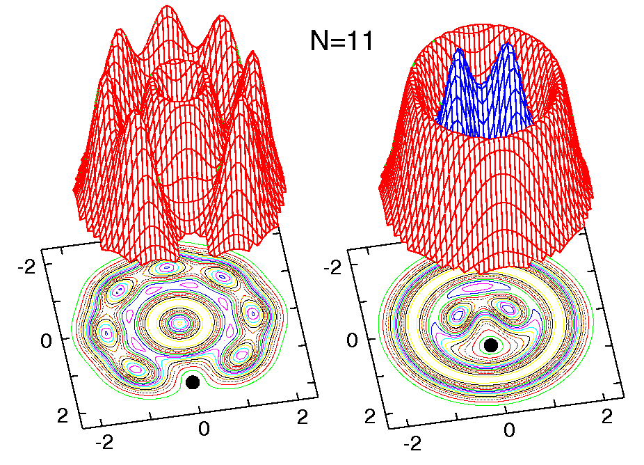
Figure 22: (Color online) Conditional probability distributions for the REM ground state of $N=11$ electrons at $B=10$ T ($L=106$). The electrons are arranged in a (3,8) structure. The observation point (solid dot) is placed on (left) the outer ring at $r_{0}=1.480R_{0}$, and (right) on the inner ring at $r_{0}=0.557R_{0}$. Parameters used: confinement $\hbar\omega_{0}=3.60$ meV, dielectric constant $\kappa=13.1$, effective mass $m^{*}=0.067m_{e}$. Lengths in units of $R_{0}=(2e^{2}/m^{*}\kappa\omega_{0}^{2})^{1/3}$. CPDs (vertical axes) in arbitrary units.

In addition to the overestimation of the ground-state energy values for smaller magnetic fields (see figure 21 and our discussion above), there are additional shortcomings of the lowest-Landau-level approximation pertaining to the ground-state ring configurations. In particular, for $N=11$, we find that according to the LLL approximation the ground-state angular momentum immediately after the maximum density droplet ($L_{0}=55$) is $L_{m}=66$, i.e., the one associated with the $(0,N)$ vortex-in-the-center configuration. This result, erroneously stated in Refs. [242, 243] as the ground state, disagrees with the correct result that includes the full effect of the confinement and is listed in table 3, where the ground-state angular momentum immediately following the maximum density droplet is $L_{m}=63$. This angular-momentum value corresponds to the classicaly most stable (3,8) ring configuration, that is, a configuration with no vortex at all (see also the case of $N=9$ electrons in Ref. [53]).

Figure 22 displays the REM conditional probability distributions for the ground state of $N=11$ electrons at $B=10$ T ($L_{m}=106$). The (3,8) ring configuration is clearly visible. We note that when the observation point is placed on the outer ring (left panel), the CPD reveals the crystalline structure of this ring only; the inner ring appears to have a uniform density. To reveal the crystalline structure of the inner ring, the observation point must be placed on this ring; then the outer ring appears to be uniform in density. This behavior suggests that the two rings rotate independently of each other, a property that is explored in the next section to derive an approximate quasiclassical expression for the yrast rotational spectra associated with an arbitrary number of electrons.

7.3 Approximate analytic expression for the yrast-band spectra

In figure 23, we display the CPD for the REM wave function of $N=17$ electrons. This case has a nontrivial three-ring structure (1,6,10) [114] which is sufficiently complex to allow generalizations for larger numbers of particles. The remarkable floppy character (leading to a non-classical, non-rigid rotational inertia, see section VI of Ref. [53]) of the REM is illustrated in the CPDs of figure 23. Indeed, as the two CPDs [reflecting the choice of taking the observation point [${\bf r}_{0}$ in (1.1)] on the outer (left frame) or the inner ring (right frame)] reveal, the polygonal electron rings rotate independently of each other. Thus, e.g., to an observer located on the inner ring, the outer ring will appear as having a uniform density, and vice versa. The wave functions obtained from exact diagonalization exhibit also the property of independently rotating rings [see, e.g., the $N=12$ and $L=132$ ($\nu=1/2$) case in figure 24], which is a testimony to the ability of the REM wave function to capture the essential physics of a finite number of electrons in high $B$. In particular, the conditional probability distribution displayed in figure 24 for exact-diagonalization wave functions exhibits the characteristics expected from the CPD evaluated using REM wave functions for the (3,9) configuration and with an angular-momentum decomposition into shell contributions [see Equation (2.25) and Equation (2.27)] $L_{1}=3+3k_{1}$ and $L_{2}=63+9k_{2}$ ($L_{1}+L_{2}=L_{m}$; for $L_{m}=132$ the angular-momentum decomposition is $L_{1}=6$ and $L_{2}=126$).

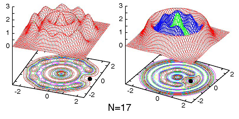
Figure 23: (Color online) Ground-state conditional probability distributions obtained from REM wave functions for the ground state of $N=17$ electrons at $B=10$ T ($L=228$). The electrons are arranged in a (1,6,10) structure. The observation point (solid dot) is placed on the outer ring at $r_{0}=1.858R_{0}$ (left frame), and on the inner ring at $r_{0}=0.969R_{0}$ (right frame). The rest of the parameters are: confinement $\hbar\omega_{0}=3.6$ meV, dielectric constant $\kappa=13.1$, effective mass $m^{*}=0.067m_{e}$. Lengths in units of $R_{0}=(2e^{2}/(\kappa m^{*}\omega_{0}^{2}))^{1/3}$. CPDs (vertical axes) in arbitrary units.

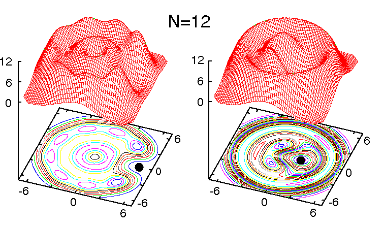
Figure 24: (Color online) CPDs for $N=12$ electrons and with angular momentum $L=132$ ($\nu=1/2$) calculated using exact diagonalization in the lowest Landau level. The electrons are arranged in a (3,9) structure. The observation point (solid dot) is placed on the outer ring at $r_{0}=5.22l_{B}$ (left frame), and on the inner ring at $r_{0}=1.87l_{B}$ (right frame). Lengths in units of $l_{B}$. CPDs (vertical axes) in arbitrary units.

In addition to the conditional probabilities, the floppy-rotor character of the REM is revealed in its excited rotational spectrum for a given $B$. From our microscopic calculations based on the wave function in (2.25), we have derived (see below) an approximate (denoted as “app”), but analytic and parameter-free, expression [see (7.7) below] which reflects directly the nonrigid character of the REM for arbitrary size. This expression allows calculation of the energies of REMs for arbitrary $N$, given the corresponding equilibrium configuration of confined classical point charges.

We focus on the description of the yrast band at a given $B$. Motivated by the aforementioned nonrigid character of the rotating electron molecule, we consider the following kinetic-energy term corresponding to a $(n_{1},\ldots,n_{q},\ldots,n_{r})$ configuration (with $\sum_{q=1}^{r}n_{q}=N$):

$$E_{\rm{app}}^{\rm{kin}}(N)=\sum_{q=1}^{r}\hbar^{2}L_{q}^{2}/(2{\cal J}_{q}(a_{q}))-\hbar\omega_{c}L/2,$$ (7.2)

where $L_{q}$ is the partial angular momentum associated with the $q$th ring about the center of the dot and the total angular momentum is $L=\sum_{q=1}^{r}L_{q}$. ${\cal J}_{q}(a_{q}))\equiv n_{q}m^{*}a_{q}^{2}$ is the rotational moment of inertia of each individual ring, i.e., the moment of inertia of $n_{q}$ classical point charges on the $q$th polygonal ring of radius $a_{q}$. To obtain the total energy, $E_{L}^{\rm{REM}}$, we include also the term $E_{\rm{app}}^{\rm{hc}}(N)=\sum_{q=1}^{r}{\cal J}_{q}(a_{q})\tilde{\omega}^{2}/2$ due to the effective harmonic confinement $\tilde{\omega}$ (see Appendix A.1), as well as the interaction energy $E_{\rm{app}}^{C}$,

$$E_{\rm{app}}^{C}(N)=\sum_{q=1}^{r}\frac{n_{q}S_{q}}{4}\frac{e^{2}}{\kappa a_{q}}+\sum_{q=1}^{r-1}\sum_{s>q}^{r}V_{C}(a_{q},a_{s}).$$ (7.3)

The first term is the intra-ring Coulomb-repulsion energy of $n_{q}$ point-like electrons on a given ring, with a structure factor

$$S_{q}=\sum_{j=2}^{n_{q}}(\sin[(j-1)\pi/n_{q}])^{-1}.$$ (7.4)

The second term is the inter-ring Coulomb-repulsion energy between rings of uniform charge distribution corresponding to the specified numbers of electrons on the polygonal rings. The expression fo $V_{C}$ is

$$V_{C}(a_{q},a_{s})=n_{q}{n_{s}}e^{2}[\kappa(a_{q}^{2}+a_{s}^{2})^{1/2}]^{-1}\;{{}_{2}F_{1}}[3/4,1/4;1;4a_{q}^{2}a_{s}^{2}(a_{q}^{2}+a_{s}^{2})^{-2}],$$ (7.5)

where ${{}_{2}F_{1}}$ is the hypergeometric function.

For large $L$ (and/or $B$), the radii of the rings of the rotating molecule can be found by neglecting the interaction term in the total approximate energy, thus minimizing only $E_{\rm{app}}^{\rm{kin}}(N)+E_{\rm{app}}^{\rm{hc}}(N)$. One finds

$$a_{q}=\lambda\sqrt{L_{q}/n_{q}},$$ (7.6)

with $\lambda=\tilde{l}=\sqrt{\hbar/m^{*}\tilde{\omega}}$; i.e., the ring radii depend on the partial angular momentum $L_{q}$, reflecting the lack of radial rigidity. Substitution into the above expressions for $E_{\rm{app}}^{\rm{kin}}$, $E_{\rm{app}}^{\rm{hc}}$, and $E_{\rm{app}}^{C}$ yields for the total approximate energy the final expression:

$$E_{\rm{app},L}^{\rm{REM}}(N)=\hbar(\tilde{\omega}-\omega_{c}/2)L+\sum_{q=1}^{r}\frac{C_{V,q}}{L_{q}^{1/2}}+\sum_{q=1}^{r-1}\sum_{s>q}^{r}V_{C}(\lambda\sqrt{\frac{L_{q}}{n_{q}}},\lambda\sqrt{\frac{L_{s}}{n_{s}}}),$$ (7.7)

where the constants

$$C_{V,q}=0.25n_{q}^{3/2}S_{q}e^{2}/(\kappa\lambda).$$ (7.8)

For simpler $(0,N)$ and $(1,N-1)$ ring configurations, Equation (7.7) reduces to the expressions reported earlier [51, 128].

The floppy-rotor character of the REM under strong magnetic field is reflected in the absence in (7.7) of a kinetic-energy term proportional to $L^{2}$. This contrasts with the rigid-rotor behavior of an electron molecule at zero magnetic field (see section 5.2 and Ref. [51]).

7.4 Possible implications for the thermodynamic limit

While our focus in this section is on the behavior of trial and exact wave functions in (finite) quantum dots in high magnetic fields, it is natural to inquire about possible implications of our findings to fractional-quantum-Hall-effect systems in the thermodynamic limit.

We recall that appropriate trial wave functions for clean FQHE systems possess a good angular momentum $L\geq L_{0}$, a property shared by both the CF/JL and REM functions [24, 55, 57, 236]. We also recall the previous finding [55, 236] that for large fractional fillings $\nu>1/7$, the liquid-like (and circularly uniform) Jastrow/Laughlin function is in the thermodynamic limit energetically favored compared to the broken-symmetry static Wigner crystal (which has no good angular momentum); for $\nu<1/7$, the static Wigner crystal becomes lower in energy. This finding was enabled by the simple form of the JL functions, which facilitated computations of total energies as a function of size for sufficiently large $N$ (e.g., $N=1000$).

A main finding of the recent literature on quantum dots is that the exact-numerical-diagonalization wave functions of small systems ($N\leq 12$) are crystalline in character for both low and high fractional fillings. This finding contradicts earlier suggestions [55, 229, 236] that, for high $\nu$’s, small systems are accurately described by the liquid-like JL wave functions and their descendants, e.g., the composite-fermion ones. Of course, for the same high $\nu$’s, our small-size results cannot exclude the possibility that the CPDs of the exact solution may exhibit with increasing $N$ a transition from crystalline to liquid character, in agreement with the JL function. However, as of now the existence of such a transition remains an open theoretical subject.

For the low fractions, the rotating-electron-molecule theory raises still another line of inquiry. Due to the specific form of the REM wave functions, computational limitations (in the so-called disk geometry that is natural to quantum dots) prevent us at present from making extrapolations of total energies at a given $\nu$ as $N\rightarrow\infty$. Nevertheless, from the general theory of projection operators, one can conclude that the REM energies exhibit a different trend compared to the JL ones, whose energies were found [55, 236] to be higher than the static Wigner crystal. Indeed the rotating-electron-molecule wave functions remain lower in energy than the corresponding static crystalline state for all values of $N$ and $\nu$, even in the thermodynamic limit. This is due to an “energy gain” theorem (see Section 3 in Ref. [241]) stating that at least one of the projected states (i.e., the ground state) has an energy lower than that of the original broken-symmetry trial function (e.g., the UHF determinant), and this theorem applies for any number of electrons $N$ and for all values of the magnetic field $B$. Naturally, the REM wave functions will be physically relevant compared to those of the broken-symmetry crystal at the thermodynamic limit if the energy gain does not vanish when $N\rightarrow\infty$; otherwise, one needs to consider the posssibility that the static crystal is the relevant physical picture.

Figure 25: Stabilization energies $\Delta E^{\rm{gain}}_{\rm{gs}}=E^{\rm{gs}}_{\rm{REM}}-E_{\rm{UHF}}$ for $N=6$ (dashed curve) and $N=7$ (solid curve) fully polarized electrons in a parabolic QD as a function of $B$. The troughs associated with the major fractional fillings (1/3, 1/5, and 1/7) and the corresponding ground-state angular momenta [$L=N(N-1)/(2\nu)$] are indicated with arrows. We have extended the calculations up to $B=120$ T (not shown), and verified that $\Delta E^{\rm{gain}}_{\rm{gs}}$ remains negative while its absolute value vanishes as $B\rightarrow\infty$. The choice of parameters is: $\hbar\omega_{0}=3$ meV (parabolic confinment), $m^{*}=0.067m_{e}$ (electron effective mass), and $\kappa=12.9$ (dielectric constant).

The discussion in the above paragraph may be recapitulated by the following question: which state is the relevant one in the thermodynamic limit $(N\rightarrow\infty)$ – the broken-symmetry one (i.e., the static crystal) or the symmetry restored (i.e., rotating crystal) state? This question, in the context of bulk broken-symmetry systems, has been addressed in the early work of Anderson [10] who concluded that the broken-symmetry state (here the UHF static crystalline solution) can be safely taken as the effective ground state. In arriving at this conclusion Anderson invoked the concept of (generalized) rigidity. As a concrete example, one would expect a crystal to behave like a macroscopic body, whose Hamiltonian is that of a heavy rigid rotor with a low-energy excitation spectrum $L^{2}/2{\cal J}$, the moment of inertia ${\cal J}$ being of order $N$ (macroscopically large when $N\rightarrow\infty$). The low-energy excitation spectrum of this heavy rigid rotor above the ground-state ($L=0$) is essentially gapless (i.e., continuous). Thus although the formal ground state posseses continuous rotational symmetry (i.e., $L=0$), “there is a manifold of other states, degenerate in the $N\rightarrow\infty$ limit, which can be recombined to give a very stable wave packet with essentially the nature” [10] of the broken-symmetry state (i.e., the static Wigner crystal in our case). As a consequence of the “macroscopic heaviness” as $N\rightarrow\infty$, one has: (I) The energy gain due to symmetry restoration (i.e., the stabilization energy $\Delta E^{\rm{gain}}_{\rm{gs}}=E^{\rm{gs}}_{\rm{REM}}-E_{\rm{UHF}}$, see figure 25) vanishes as $N\rightarrow\infty$, and (II) The relaxation of the system from the wave packet state (i.e., the static Wigner crystal) to the symmetrized one (i.e., the rotating crystal) becomes exceedingly long. This picture underlies Anderson’s aforementioned conclusion that in the thermodynamic limit the broken-symmetry state may be used as the effective ground state.

Consequently, in the rest of this section we will focus on issues pertaining to the “rigidity” of the rotating electron molecule in high magnetic fields. In particular, using our projection method and exact diagonalization, we have demonstrated explicitly [50, 51] that the rigid-rotor picture applies to an $N$-electron QD only when $B=0$. In contrast, in the presence of a high magnetic field, we found [51, 52, 53] that the electrons in the quantum dot do not exhibit global rigidity and therefore cannot be modeled as a macroscopic rotating crystal. Instead, a more appropriate model is that of a highly non-rigid rotor whose moment of inertia depends strongly on the value of the angular momentum $L$. This behavior originates from the dominance of the magnetic field over the Coulomb repulsion.

The non-rigid rotor at high $B$ has several unique properties: (I) The ground state has angular momentum $L_{\rm{gs}}>0$; (II) While the rotating electron molecule does not exhibit global rigidity, it possesses azimuthal rigidity (i.e., all electrons on a given ring rotate coherently), with the rings, however, rotating independently of each other. Furthermore, the radii of the rings vary for different values of $L$, unlike the case of a rigid rotor; (III) The excitation spectra do not vary as $L^{2}$; instead they consist of terms that vary as $aL+\sum_{q=1}^{r}b_{q}/\sqrt{L_{q}}$ (with $\sum_{q=1}^{r}L_{q}=L$; for the precise values of the constants $a$ and $b$ see section 7.3 and Refs. [51, 53]); (IV) The angular momentum values are given by the magic values [see section 6.1] $L=L_{0}+\sum_{q=1}^{r}k_{q}n_{q}$, where $(n_{1},n_{2},\ldots,n_{r})$ is the polygonal ring arrangement of the static Wigner molecule (with $n_{q}$ the number of electrons on the $q$th ring) and $k_{1}<k_{2}<\ldots<k_{q}$ are nonnegative integers. These magic $L$’s are associated with the cusp states which exhibit a relative energy gain with respect to neighboring excitations. Thus the low-energy excitation spectrum of the non-rigid rotor is not dense and exhibits gaps due to the occurrence of the magic (cusp) states (see figure 26). Furthermore, these gaps are reflected in the oscillatory behavior of $\Delta E^{\rm{gain}}_{\rm{gs}}$ (see, e.g., figure 25) as a function of $B$ (or $\nu$).

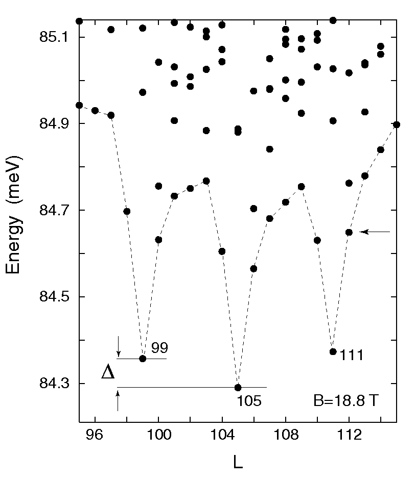
Figure 26: Low-energy part of the spectrum of the parabolic QD whose parameters are the same as those in figure 25, calculated as a function of the angular momentum $L$ through exact diagonalization for $N=7$ electrons at a magnetic field $B=18.8$ T. We show here the spectrum in the interval $95\leq L\leq 115$ (in the neighborhood of $\nu=1/5$). The magic angular momentum values corresponding to cusp states are marked (99, 105, and 111), and they are seen to be separated from the rest of the spectrum. For the given value of $B$, the global energy minimum (ground state) occurs for $L_{\rm{gs}}=105$, and the gap $\Delta$ to the first excited state ($L=99$) is indicated. The lowest energies for the different $L$’s (the yrast band) in the plotted range are connected by a dashed line, as a guide to the eye. The zero of energy corresponds to $7\hbar\tilde{\omega}$, where $\tilde{\omega}=(\omega_{0}^{2}+\omega_{c}^{2}/4)^{1/2}$ and $\omega_{c}=eB/(m^{*}c)$. The horizontal arrow denotes the energy of the Laughlin quasihole at L=112. It is seen that the Laughlin quasihole is not the lowest excited state, as presumed in Ref. [55].

As $N$ increases, more polygonal rings are successively added, and since the polygonal rings rotate independently of each other (see, e.g., the case of $N=12$ in figure 24), we expect that the non-rigid-rotor picture remains valid even as $N\rightarrow\infty$. As a result, it is plausible to conjecture the following properties at high $B$ in the thermodynamic limit: (I) the oscillatory character of $\Delta E^{\rm{gain}}_{\rm{gs}}$ will maintain, yielding nonvanishing stabilization energies at the fractional fillings $\nu$, and (II) the low-energy excitation spectra of the system will still exhibit gaps in the neighborhood of the magic angular momenta (see figure 26). Of course, these conjectures need to be further supported through numerical calculations for large $N$. Nevertheless, the above discussion indicates that the question of which state is physically relevant for low fractions in the thermodynamic limit at high $B$ – i.e., the broken-symmetry static crystal or the symmetrized rotating crystal – remains open, and cannot be answered solely following the path of Anderson as described in Ref. [10].

The rotating Wigner crystal has properties characteristic of FQHE states, i.e., it is incompressible (connected to the presence of an excitation gap) and carries a current (while the broken-symmetry static crystal is insulating). Thus, we may conjecture that a transition at lower fractional fillings from a conducting state with good circular symmetry to an insulating Wigner crystal cannot occur spontaneously for clean systems. Therefore, it should be possible to observe FQHE-type behavior at low fractional fillings in a clean system – a prediction that could explain the observations of Ref. [244], where FQHE behavior has been observed for low fractional fillings typically associated with the formation of a static Wigner crystal. In practice, however, impurities and defects may influence the properties of the rotating crystal (and its excitations), depending on the magnitude of the excitation gap (see, e.g., figure 26). Thus one of the main challenges for observation of the fractional quantum Hall effect at such low fillings relates to fabrication of high mobility (nearly impurity-free) samples [245]. We remark, however, that the stabilization energy and the gap $\Delta$ (see, e.g., figure 26) diminish as the magnetic field increases, and as a result the impurities become more efficient in influencing the rotating Wigner crystal for the lower fractional fillings (i.e., higher angular momenta).

8 Bosonic molecules in rotating traps: Original results and applications

8.1 Variational description of rotating boson molecules

Recent experimental advances in the field of trapped ultracold neutral bosonic gases have enabled control of the strength of interatomic interactions over wide ranges [85, 86, 87, 246], from the very weak to the very strong. This control is essential for experimental realizations of novel states of matter beyond the well known Bose-Einstein condensate [85, 86, 87]. In this context, the linear 1D Tonks-Girardeau regime of impenetrable trapped bosons has generated intensive theoretical activity [247, 248] and several experimental realizations of it have been reported most recently [85, 86].

In this section, we address the properties of strongly-repelling impenetrable bosons in rotating ring-shaped or 2D harmonic traps. It has been found that impenetrable bosons are “localized” relative to each other [60, 63, 85] and exhibit nontrivial intrinsic crystalline correlations [60, 63]. For a small number of bosons, $N$, these crystalline arrangements are reminiscent of the structures exibited by the well-studied rotating electron molecules in quantum dots under high magnetic fields [26, 52, 53]. Consequently, we use in the following the term rotating boson molecules. A central result of our study is that the point-group symmetries of the intrinsic crystalline structures give rise to characteristic regular patterns (see below) in the ground-state spectra and associated angular momenta of the RBMs as a function of the rotational frequency for neutral bosons (or the magnetic field for charged bosons).

An unexpected result of our studies is that the rotation of repelling bosons (even those interacting weakly) does not necessarily lead to formation of vortices, as is familiar from the case of rotating Bose-Einstein condenstates. In particular, for small $N$, we will show that the Gross-Pitaevskii energies (including those corresponding to formation of vortices) remain always higher compared to the ground-state energies of the RBMs. Of course, we expect that the rotating BEC will become the preferred ground state for sufficiently large $N$ in the case of weakly repelling neutral bosons. We anticipate, however, that it will be feasible to test our unexpected results for small $N$ by using rotating optical lattices, where it is established that a small finite number of atoms can be trapped per given site [87].

In a non-rotating trap, it is natural to describe a localized boson (at a position ${\bf R}_{j}$) by a simple displaced Gaussian [60]. When the rotation of the trap is considered, the Gaussian needs to be modified by a phase factor, determined through the analogy between the one-boson Hamiltonian in the rotating frame of reference and the planar motion of a charged particle under the influence of a perpendicular magnetic field $B$ (described in the symmetric gauge). That is, the single-particle wave function of a localized boson is

$$\varphi_{j}({\bf r})\equiv\varphi({\bf r},{\bf R}_{j})=\frac{1}{\sqrt{\pi}\lambda}\exp\left[\frac{({\bf r}-{\bf R}_{j})^{2}}{2\lambda^{2}}-\rmi{\bf r}{\bf\cdot}({\bf Q}\times{\bf R}_{j})\right],$$ (8.1)

with ${\bf Q}\equiv{\bf\hat{z}}/\Lambda^{2}$ and the width of the Gaussian $\lambda$ is a variational parameter; $\Lambda\equiv l_{B}\sqrt{2}=\sqrt{2\hbar c/(eB)}=\sqrt{2\hbar/(m\omega_{c})}$ for the case of a perpendicular magnetic field ${\bf B}$, and $\Lambda\equiv l_{\Omega}\sqrt{2}=\sqrt{\hbar/(m\Omega)}$ in the case of a rotating trap with rotational frequency ${\bf\Omega}$ (we recall that $\omega_{c}\rightarrow 2\Omega$, see the Appendix). Note that we consider a 2D trap, so that ${\bf r}\equiv(x,y)$ and ${\bf R}\equiv(X,Y)$.

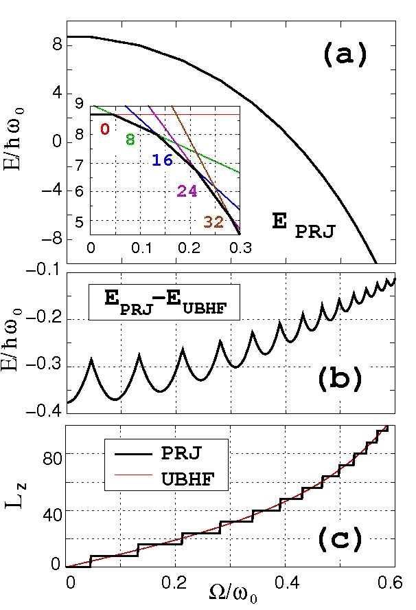
Figure 27: (Color online) Properties of $N=8$ neutral repelling bosons in a rotating toroidal trap as a function of the reduced rotational frequency $\Omega/\omega_{0}$. The confining potential is given by (8.4) with $n=2$ and radius $r_{0}=3l_{0}$, and the interaction-strength parameter was chosen as $R_{\delta}=50$. (a) RBM ground-state energies, $E^{\rm{PRJ}}$. The inset shows the range $0\leq\Omega/\omega_{0}\leq 0.3$. The numbers denote ground-state magic angular momenta. (b) Energy difference $E^{\rm{PRJ}}-E^{\rm{UBHF}}$. (c) Total angular momenta associated with (i) the RBM ground states [thick solid line (showing steps and marked as PRJ); online black] and (ii) the UBHF solutions (thin solid line; online red). In the figures, we may use the symbol $L_{z}$, instead of simply $L$, to denote the 2D total angular momentum.

The Hamiltonian corresponding to the single-particle kinetic energy is given by

$$H_{K}({\bf r})=({\bf p}-\hbar{\bf Q}\times{\bf r})^{2}/(2m),$$ (8.2)

for the case of a magnetic field, and by

$$H_{K}({\bf r})=({\bf p}-\hbar{\bf Q}\times{\bf r})^{2}/(2m)-m\Omega^{2}{\bf r}^{2}/2,$$ (8.3)

for the case of a rotating frame of reference.

A toroidal trap with radius $r_{0}$ can be specified by the confining potential

$$V({\bf r})=\frac{\hbar\omega_{0}}{2}(r-r_{0})^{n}/l_{0}^{n},$$ (8.4)

with $l_{0}=\sqrt{\hbar/(m\omega_{0})}$ being the characteristic length of the 2D trap. For $n\gg 2$ and $l_{0}/r_{0}\to 0$ this potential approaches the limit of a toroidal trap with zero width, which has been considered often in previous theoretical studies (see, e.g., Ref. [249]). In the following, we consider the case with $n=2$, which is more realistic from the experimental point of view. In this case, in the limit $r_{0}=0$, one recovers a harmonic trapping potential.

To construct an RBM variational many-body wave function describing $N$ impenetrable bosons in the toroidal trap, we use $N$ displaced orbitals $\varphi({\bf r},{\bf R}_{i})$, $i=1,2,\ldots,N$ [see (8.1)] centered at the vertices of a regular polygon. Then, we first construct an unrestricted Bose Hartree-Fock permanent [60, 63] $|\Phi^{\rm{UBHF}}_{N}\rangle\propto\sum_{P(i_{m})}\varphi_{1}({\bf r}_{i_{1}})\varphi_{2}({\bf r}_{i_{2}})\ldots\varphi_{N}({\bf r}_{i_{N}})$. The UBHF permanent breaks the circular symmetry of the many-body Hamiltonian. As was discussed in section 3.2, the “symmetry dilemma” is resolved through a subsequent “symmetry-restoration” step accomplished via projection techniques [23, 24, 30, 31, 52, 53], i.e., we construct a many-body wave function with good total angular momentum by applying the projection operator $\hat{\cal P}_{L}=(1/2\pi)\int_{0}^{2\pi}\rmd\theta\exp[\rmi\theta(L-\hat{L})]$, so that the final RBM wave function is given by

$$|\Psi^{\rm{PRJ}}_{N,L}\rangle=\frac{1}{2\pi}\int_{0}^{2\pi}\rmd\theta|\Phi^{\rm{UBHF}}_{N}(\theta)\rangle\rme^{\rmi\theta L}.$$ (8.5)

$|\Phi^{\rm{UBHF}}_{N}(\theta)\rangle$ is the original UBHF permanent rotated by an azimuthal angle $\theta$. We note that, in addition to having good angular momenta, the projected wave function $|\Psi^{\rm{PRJ}}_{N,L}\rangle$ has also a lower energy than that of $|\Phi^{\rm{UBHF}}_{N}\rangle$ [see, e.g. $E_{L}^{\rm{PRJ}}-E^{\rm{UBHF}}$ in figure 27(b). The projected ground-state energy is given by

$$E_{L}^{\rm{PRJ}}=\int_{0}^{2\pi}h(\theta)\rme^{\rmi\theta L}\rmd\theta\left/\int_{0}^{2\pi}n(\theta)\rme^{\rmi\theta L}\right.\rmd\theta,$$ (8.6)

where $h(\theta)=\langle\Phi_{N}^{\rm{UBHF}}(\theta=0)|{\cal H}|\Phi_{N}^{\rm{UBHF}}(\theta)\rangle$ and $n(\theta)=\langle\Phi_{N}^{\rm{UBHF}}(\theta=0)|\Phi_{N}^{\rm{UBHF}}(\theta)\rangle$; the latter term ensures proper normalization.

Figure 28: (Color online) Single-particle densities and CPDs for $N=8$ bosons in a rotating toroidal trap with $\Omega/\omega_{0}=0.2$ and $R_{\delta}=50$. The remaining trap parameters are as in figure 27. (a) Gross-Pitaevskii single-particle density. (b) UBHF single-particle density exhibiting breaking of the circular symmetry. (c) RBM single-particle density exhibiting circular symmetry. (d) CPD for the RBM wave function [PRJ wave function, see Equation (8.5)] revealing the hidden point-group symmetry in the intrinsic frame of reference. The observation point is denoted by a white dot. The RBM ground-state angular momentum is $L_{z}=16$. Lengths in units of $l_{0}$. The vertical scale is the same for (b), (c), and (d), but different for (a).

The many-body Hamiltonian in the rotating trap is given by

$${\cal H}=\sum_{i=1}^{N}[H_{K}({\bf r}_{i})+V({\bf r}_{i})]+\sum_{i<j}^{N}v({\bf r}_{i},{\bf r}_{j}),$$ (8.7)

with the interparticle interaction being given by a contact potential $v_{\delta}({\bf r}_{i},{\bf r}_{j})=g\delta({\bf r}_{i}-{\bf r}_{j})$ for neutral bosons and a Coulomb potential $v_{C}({\bf r}_{i},{\bf r}_{j})=Z^{2}e^{2}/|{\bf r}_{i}-{\bf r}_{j}|$ for charged bosons. The parameter that controls the strength of the interparticle repulsion relative to the zero-point kinetic energy is given by $R_{\delta}=gm/(2\pi\hbar^{2})$ [60, 63] for a contact potential and $R_{W}=Z^{2}e^{2}/(\hbar\omega_{0}l_{0})$ [20, 60] for a Coulomb repulsion.

For a given value of the dimensionless rotational frequency, $\Omega/\omega_{0}$, the projection yields wave functions and energies for a whole rotational band comprising many angular momenta. In the following, we focus on the ground-state wave function (and corresponding angular momentum and energy) associated with the lowest energy in the band.

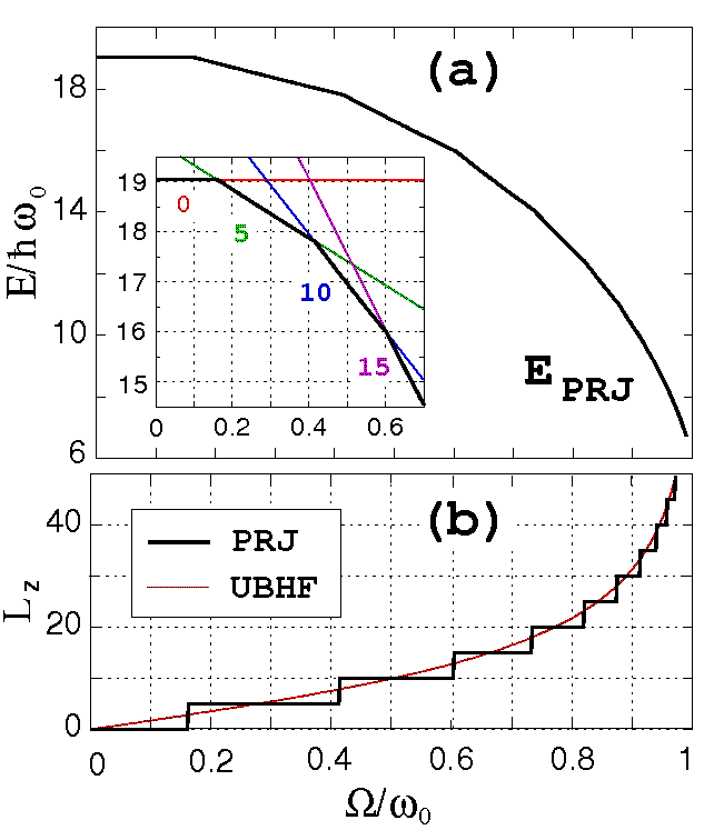
Figure 29: (Color online) Properties of $N=6$ neutral bosons in a rotating harmonic trap as a function of the reduced rotational frequency $\Omega/\omega_{0}$. The confining potential is given by (8.4) with $n=2$ and $r_{0}=0$, and the interaction-strength parameter was chosen as $R_{\delta}=50$. The intrinsic molecular structure is $(1,5)$. (a) RBM ground-state energies, $E^{\rm{PRJ}}$. The inset shows a smaller range. The numbers denote ground-state angular momenta. (b) Total angular momenta associated with (i) the RBM ground states (thick solid line showing steps; online black) and (ii) the UBHF solutions (thin solid line; online red).

Figure 27(a) displays the ground-state energy $E_{\rm{PRJ}}$ of $N=8$ bosons in a toroidal trap as a function of the dimensionless rotational frequency $\Omega/\omega_{0}$, with $\omega_{0}$ being the trap frequency. The prominent features in figure 27(a) are: (i) the energy diminishes as $\Omega/\omega_{0}$ increases; this is an effect of the centrifugal force, and (ii) the $E_{\rm{PRJ}}$ curve consists of linear segments, each one associated with a given angular momentum $L$. Most remarkable is the regular variation of the values of $L$ with a constant step of $N$ units (here $N=8$) [see inset in figure 27(a) and figure 27(c)]. These preferred angular momenta $L=kN$ with integer $k$, are reminiscent of the so called “magic angular momenta” familiar from studies of electrons under high-magnetic fields in 2D semiconductor quantum dots [26, 52, 53].

Figure 30: (Color online) Properties of GP solutions (thin solid line; online red) versus those of RBM wave functions (thick solid line; online green) for $N=6$ neutral bosons as a function of the reduced rotational frequency $\Omega/\omega_{0}$. A harmonic trap is considered, and the interaction strength equals $R_{\delta}=50$. (a) Ground-state energies. (b) Associated ground-state angular momenta. (c) GP (BEC) single-particle density at $\Omega/\omega_{0}=0.65$ having 7 vortices with a 6-fold symmetry (thus exhibiting breaking of the circular symmetry). (d) RBM single-particle density at $\Omega/\omega_{0}=0.65$ which does not break the circular symmetry. (e) CPD of the RBM at $\Omega/\omega_{0}=0.65$ revealing the intrinsic (1,5) crystalline pattern. The white dot denotes the observation point ${\bf r}_{0}$. Note the dramatic difference in spatial extent between the GP and RBM wave functions [compare (c) with (d) and (e). Lengths in units of $l_{0}$. The vertical scale is the same for (d) and (e), but different for (c).

The preferred angular momenta reflect the intrinsic molecular structure of the localized impenetrable bosons. We note, that the (0,8) polygonal-ring arrangement is obvious in the single-particle density associated with the UBHF permanent [see figure 28(b)]; (0,8) denotes no particles in the inner ring and 8 particles in the outer one. After restoration of symmetry, however, the single-particle density is circularly symmetric [see the PRJ single-particle density in figure 28(c)] and the intrinsic crystallinity becomes “hidden”; it can, however, be revealed via the conditional probability distribution [20, 52, 53, 60] [CPD, see figure 28(d)]. We note the Gross-Pitaevskii single-particle density in figure 28(a), which is clearly different from the PRJ density in figure 28(c).

The internal structure for charged bosons in a toroidal trap (not shown) is similar to that of neutral bosons (figure 28), i.e., a (0,8) ring arrangement, portrayed also in the stepwise variation (in steps of 8 units) of the total angular momenta. The internal structure is also reflected in the variation of the ground-state total energy as a function of the magnetic field. In contrast to the case of neutral bosons, however, the ground-state energy curve for charged bosons is not composed of linear segments, but of intersecting inverted-parabola-type pieces; this is due to the positive contribution of the Lorentz force compared to the negative contribution of the centrifugal force in a rotating trap.

For RBMs in rotating harmonic traps, the polygonal-ring pattern of localized bosons becomes more complex than the simple $(0,N)$ arrangement that appears naturally in a toroidal trap. Indeed, in harmonic traps, one anticipates the emergence of concentric ring structures. For $N=6$ neutral bosons in a harmonic trap, we observe that, as in the case of a toroidal trap, the ground-state energy as a function of the reduced rotational frequency, $\Omega/\omega_{0}$, [figure 29(a)] is composed of linear segments, but now the corresponding magic angular momenta [figure 29(b)] vary in steps of $N-1=5$ units. This indicates a rotating boson molecule consisting of two polygonal rings; denoted as a $(1,5)$ structure, with the inner ring having a single boson and the outer ring five.

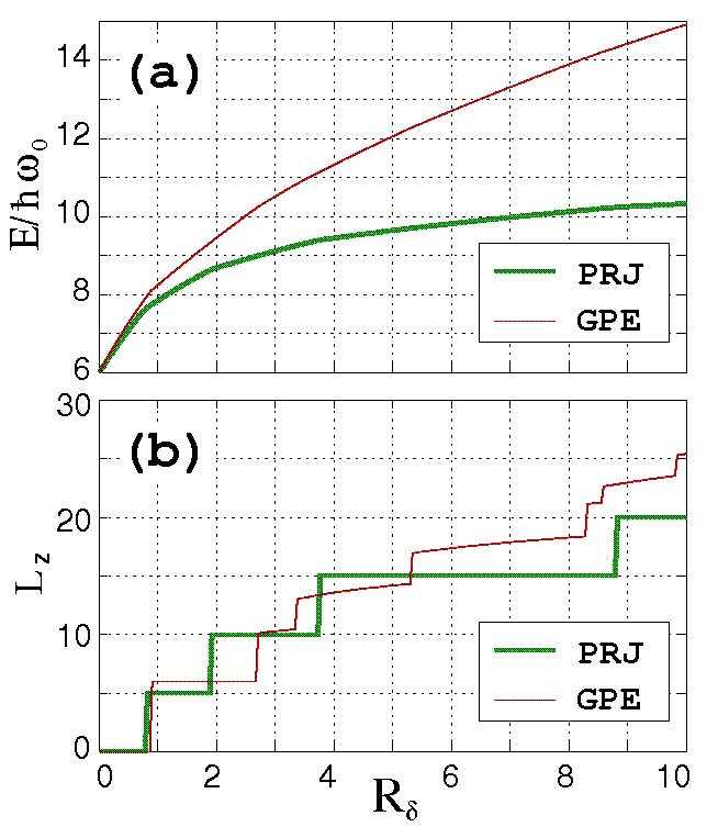
Figure 31: (Color online) Properties of GP solutions (thin solid line; online red) versus those of RBM wave functions (thick solid line; online green) for $N=6$ bosons as a function of the interaction strength $R_{\delta}$. A harmonic trap is considered, and the reduced rotational frequency equals $\Omega/\omega_{0}=0.85$. (a) Ground-state energies (b) Associated ground-state angular momenta.

In figure 30(a), we display the rotating-boson-molecule and mean-field Gross-Pitaevskii ground-state energies of $N=6$ strongly repelling (i.e., $R_{\delta}=50$) neutral bosons in a harmonic trap as a function of the reduced angular frequency of the trap. The GP curve (thin solid line; online red) remains well above the RBM curve (thick solid line; online green) in the whole range $0\leq\Omega/\omega_{0}\leq 1$. The RBM ground-state angular momenta exhibit again the periodicity in steps of five units [figure 30(b)]. As expected, the GP total angular momenta are quantized [$L_{z}=0$ (no-vortex) or $L_{z}=6$ (one central vortex)] only for an initial range $0\leq\Omega/\omega_{0}\leq 0.42$. For $\Omega/\omega_{0}\geq 0.42$, the GP total angular momentum takes non-integer values and ceases to be a good quantum number, reflecting the broken-symmetry character of the associated mean field, with each kink signaling the appearance of a different vortex pattern of $p$-fold symmetry ($p=1,2,3,4,\ldots$) [250]; see an example in figure 30(c). The energetic superiority of the RBM wave function over the GP solution demonstrated in figure 30(a) was to be expected, since we considered the case of strongly repelling bosons. Unexpectedly, however, for a small number of neutral bosons the energetic advantage of the rotating boson molecule persists even for weakly repelling bosons, as illustrated in figure 31(a). Indeed, figure 31(a) displays the RBM (thick solid line; online green) and GP (thin solid line; online red) ground-state energies for $N=6$ neutral bosons in a trap rotating with $\Omega/\omega_{0}=0.85$ as a function of the interaction parameter $R_{\delta}$. The surprising result in figure 31(a) is that the GP energy remains above the RBM curve even for $R_{\delta}\rightarrow 0$. Of course the RBM wave function is very close to that of a BEC without vortices when $R_{\delta}\rightarrow 0$ (BECs without vortices are approximately feasible for small $N$). However, for small $N$, our results show that BECs with vortices (i.e., for $L_{z}\geq N$) are not the preferred many-body ground states; instead, formation of RBMs is favored. Note that the energy difference $E^{\rm{GP}}-E^{\rm{PRJ}}$ increases rapidly with increasing $R_{\delta}$, reflecting the fact that the RBM energies saturate (as is to be expected from general arguments), while the GP energies (even with vortices fully accounted for) exhibit an unphysical divergence as $R_{\delta}\rightarrow\infty$ [figure 31(a)]; we have checked this trend up to values of $R_{\delta}=100$ (not shown). Of interest again is the different behavior of the RBM and GP ground state angular momenta [figure 31(b)] (see also discussion of figure 30(b)).

To summarize this section: We have studied the ground-state properties of a variational many-body wave function for repelling bosons in rotating traps that incorporates correlations beyond the Gross-Pitaevskii mean-field approximations. This variational wave function describes rotating boson molecules, i.e., localized bosons arranged in polygonal-ring-type patterns in their intrinsic frame of reference. For small numbers of neutral bosons, and in particular in the case of GP vortex formation, the RBM ground-state energies are lower than those associated with the corresponding Gross-Pitaevskii BEC solutions. Given the large differences between the properties of the RBM and BEC wave functions (which become more pronounced for larger interaction parameter $R_{\delta}$), and the recently demonstrated ability to experimentally control $R_{\delta}$ [85, 86, 87, 246], we anticipate that our results could be tested in experiments involving rotating optical lattices. Detection of rotating boson molecules could be based on a variety of approaches, such as the measurement of the spatial extent [contrast the RBM and BEC spatial extents in figure 30(c) - figure 30(e)], or the use of Hanbury Brown-Twiss-type experiments [251] to directly detect the intrinsic crystalline structure of the RBM.

8.2 Exact diagonalization for bosons in the lowest Landau level

Rotating ultracold trapped Bose condensed systems are most commonly discussed in the context of formation of vortex lattices, which are solutions to the Gross-Pitaevskii mean-field equation [4, 5, 252, 253, 254, 255, 256, 257]. Such vortex lattices have indeed been found experimentally for systems containing a large number of bosons [258, 259, 260]. Nevertheless, several theoretical investigations [67, 68, 69, 70, 71] of rapidly rotating trapped bosonic systems suggested formation of strongly correlated exotic states which differ drastically from the aforementioned vortex-lattice states. While experimental realizations of such strongly correlated states have not been reported yet, there is already a significant effort associated with two-dimenional exact-diagonalization studies of a small number of particles ($N$) in the lowest Landau level; the LLL restriction corresponds to the regime of rapid rotation, where the rotational frequency of the trap $\Omega$ equals the frequency of the confining potential. The large majority [67, 69, 70, 71] of such exact-diagonalization studies have attempted to establish a close connection between rapidly rotating bosonic gases and the physics of electrons under fractional-quantum-Hall-effect conditions employing the bosonic version of “quantum-liquid” analytic wave functions, such as the Laughlin wave functions, composite-fermion, Moore-Read, and Pfaffian functions.

As described in section 6, the “quantum-liquid” picture for a small number of trapped electrons in the FQHE regime has been challenged in a series of extensive studies [24, 26, 42, 51, 52, 53] of electrons in 2D quantum dots under high magnetic fields. Such studies (both exact-diagonalization and variational) revealed that, at least for finite systems, the underlying physical picture governing the behavior of strongly-correlated electrons is not that of a “quantum liquid.” Instead, the appropriate description is in terms of a “quantum crystal,” with the localized electrons arranged in polygonal concentric rings [24, 26, 51, 52, 53, 127, 128, 131]. These “crystalline” states lack [52, 53] the familiar rigidity of a classical extended crystal, and are better described [24, 26, 42, 51, 52, 53] as rotating electron (or Wigner) molecules.

Motivated by the discovery in the case of electrons of REMs at high $B$ (and from the fact that Wigner molecules form also at zero magnetic field [20, 25, 41, 50, 167, 188]) some theoretical studies have most recently shown that analogous molecular patterns of localized bosons do form in the case of a small number of particles inside a static or rotating harmonic trap [43, 60, 63, 177, 178]. In analogy with the electron case, the bosonic molecular structures can be referred to [63] as rotating boson molecules; a description of RBMs via a variational wave function built from symmetry-breaking displaced Gaussian orbitals with subsequent restoration of the rotational symmetry was presented in Refs. [43, 60, 63] and reviewed in section 8.1.

In a recent paper, Baksmaty et al[72] used exact diagonalization in the lowest Landau level to investigate the formation and properties of RBMs focusing on a larger number of particles than previously studied, in particular for sizes where multiple-ring formation can be expected based on our knowledge of the case of 2D electrons in high $B$. A finite number of particles ($N\leq 11$) at both low ($\nu<1/2$) and high ($\nu\geq 1/2$) filling fractions $\nu\equiv N(N-1)/2L$ (where $L\equiv{\cal L}/\hbar$ is the quantum number associated with the total angular momentum ${\cal L}$) was studied and both the cases of a long-range (Coulomb) and a short-range ($\delta$-function) repulsive interaction were investigated. In this section, we report some main results from Ref. [72].

As in the case of electrons in 2D quantum dots, we probe the crystalline nature of the bosonic ground states by calculating the full anisotropic two-point correlation function $P({\bf r},{\bf r}_{0})$ [see Equation (1.1)] associated with the exact wavefunction $\Psi({\bf r}_{1},{\bf r}_{2},\ldots,{\bf r}_{N})$. The quantity $P({\bf r},{\bf r}_{0})$ is proportional to the probability of finding a boson at ${\bf r}$ given that there is another boson at the observation point ${\bf r}_{0}$, and it is often referred to as the conditional probability distribution (section 1.5). A main finding of our studies is that consideration solely of the CPDs is not sufficient for the boson case at high fractional fillings $\nu\geq 1/2$; in this case, one needs to calculate even higher-order correlation functions, e.g., the full $N$-point correlation function defined as the modulus square of the full many-body EXD wave function, i.e.,

$$P({\bf r};{\bf r}_{1},{\bf r}_{2},\ldots,{\bf r}_{N-1})=|\Psi({\bf r};{\bf r}_{1},{\bf r}_{2},\ldots,{\bf r}_{N-1})|^{2},$$ (8.8)

where one fixes the positions of $N-1$ particles and inquiries about the (conditional) probability of finding the $N$th particle at any position ${\bf r}$.

The investigations in this section are also motivated by recent experimental developments, e.g., the realization of trapped ultracold gas assemblies featuring bosons interacting via a long-range dipole-dipole interaction [261, 262]. We expect the results presented in this section to be directly relevant to systems with a two-body repulsion intermediate between the Coulomb and the delta potentials. Additionally, we note the appearance of promising experimental techniques for measuring higher-order correlations in ultra-cold gases employing an atomic Hanbury Brown-Twiss scheme [251] or shot-noise interferometry [263, 264]. Experimental realization of few-boson rotating systems can be anticipated in the near future as a result of increasing sophistication of experiments involving periodic optical lattices co-rotating with the gas, which are capable of holding a few atoms in each site. A natural first step in the study of such systems is the analysis of the physical properties of a few particles confined in a rotating trap with open boundary conditions (i.e., conservation of the total angular momentum $L$).

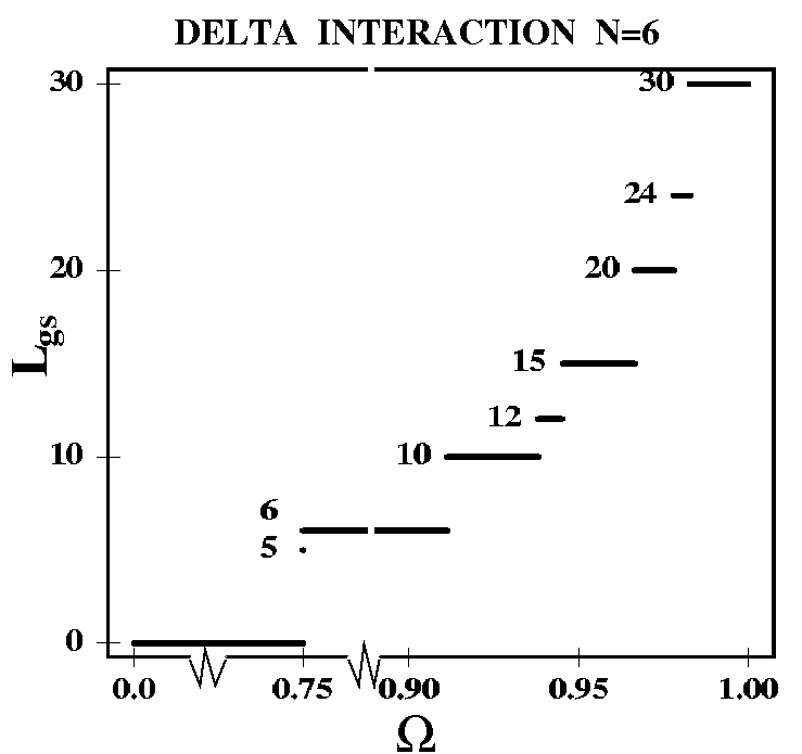
Figure 32: Ground-state angular momenta, $L_{\rm{gs}}$, for $N=6$ bosons in a rapidly rotating trap [described by the LLL Hamiltonian in (8.9)], as a function of the rotational frequency $\Omega$ expressed in units of $\omega_{0}$. The bosons interact via a Coulombic repulsion (left) and a delta repulsion (right), and the many-body Hilbert space is restricted to the lowest Landau level. The angular momentum associated with the first bosonic Laughlin state occurs at $L=30$, i.e., at $N(N-1)$. The value of $c=0.2\hbar\omega_{0}\Lambda$ for the Coulomb case (left) and the value of $g=2\pi\hbar\omega_{0}\Lambda^{2}/N$ for the case of a delta repulsion (right); the many-body wave functions do not depend on these choices. In the delta-interaction case, the values of the angular momenta terminate with the value $L=30$ (the Laughlin value) at $\Omega/\omega_{0}=1$. In contrast, in the Coulomb-interaction case (left), the values of the ground-state angular momenta do not terminate, but diverge as $\Omega/\omega_{0}\rightarrow 1$. Note the stepwise variation of the values of the ground-state angular momenta in both cases, indicating the presence of an intrinsic point-group symmetry associated with the (0,6) and (1,5) polygonal-ring structure of a rotating Boson molecule.

The main results of Ref. [72] can be summarized as follows: Similar to the well-established (see section 6 and section 7) emergence of rotating electron molecules in quantum dots, rotating boson molecules form in rotating harmonic traps as well. The RBMs are also organized in concentric polygonal rings that rotate independently of each other, and the polygonal rings correspond to classical equilibrium configurations and/or their low-energy isomers. Furthermore, the degree of crystallinity increases gradually with larger angular momenta $L$’s (smaller filling fractions $\nu$’s), as was the trend [26, 52, 53] for the REMs and as was observed also for $\nu<1/2$ in another study [178] for rotating bosons in the lowest Landau level with smaller $N$ and single-ring structures. We finally note that the crystalline character of the RBMs appears to depend only weakly on the range of the repelling interaction, for both the low (see also Ref. [178]) and high (unlike Ref. [177]) fractional fillings.

In studies of 2D quantum dots, CPDs were used some time ago in Refs. [50, 128, 131]. For probing the intrinsic molecular structure in the case of ultracold bosons in 2D traps, however, they were introduced only recently by Romanovsky et al[60]. The importance of using CPDs as a probe can hardly be underestimated. Indeed, while exact-diagonalization calculations for bosons in the lowest Landau level have been reported earlier [67, 68, 69, 70, 71], the analysis in these studies did not include calculations of the CPDs, and consequently formation of rotating boson molecules was not recognized.

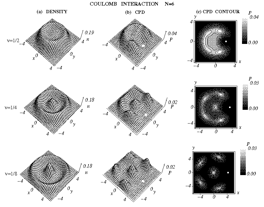
Figure 33: (a) Single-particle densities [$n({\bf r})$; left column], (b) CPDs $\left[P({\bf r},{\bf r}_{0})\right]$ in 3D plots (middle column), and (c) CPDs in contour plots (right column), portraying the strengthening of the crystalline RBM structure for $N=6$ bosons interacting via a repulsive Coulomb interaction as the filling fraction $\nu$ is reduced. The white dots in the CPD plots indicate the reference point ${\bf r}_{0}$. We note in particular the gradual enhancement of the peak at the center of the plots, and the growth of the radius of the outer ring; the latter reflects the nonrigid-rotor nature of the RBMs (in analogy with the findings of Ref. [52] regarding the properties of rotating electron molecules). The cases of $\nu=1/4$ and $\nu=1/8$ exhibit a clear $(1,5)$ crystalline arrangement, while the case of $\nu=1/2$ (first Laughlin state) is intermediate between a $(1,5)$ and a $(0,6)$ pattern (see text for details). Lengths in units of $\Lambda$. The vertical scales are in arbitrary units, which however do not change for the panels within the same column (a), (b), or (c).

8.2.1 The case of $N=6$ bosons in the lowest Landau level.

As a specific example of the points discussed above in section 8.2, we present here results for $N=6$ bosons in the lowest Landau level. For additional cases (e.g., $N=9$ and $N=11$), see Ref. [72].

In analogy with the magnetic-field Hamiltonian of Equation (7.1), the many-body Hamiltonian for $N$ bosons in a rotating trap is reduced in the lowest Landau level to the expression

$$\tilde{\cal H}^{\Omega}_{\rm{LLL}}=N\hbar\omega_{0}+\hbar(\omega_{0}-\Omega)L+\sum_{i<j}^{N}v({\bf r}_{i},{\bf r}_{j}),$$ (8.9)

where $\omega_{0}$ specifies the 2D harmonic trap and $\Omega$ denotes the rotational frequency. The interparticle interaction is given by a contact potential $v_{\delta}({\bf r}_{i},{\bf r}_{j})=g\delta({\bf r}_{i}-{\bf r}_{j})$ for neutral bosons and a Coulomb potential $v_{C}({\bf r}_{i},{\bf r}_{j})=c/|{\bf r}_{i}-{\bf r}_{j}|$ for charged bosons.

Since $\tilde{\cal H}^{\Omega}_{\rm{LLL}}$ is rotationally invariant, i.e., $[\tilde{\cal H}^{\Omega}_{\rm{LLL}},L]=0$, its eigenstates $\Psi_{L}$ must also be eigenstates of the total angular momentum with eigenvalue $\hbar L$. For a given rotational frequency $\Omega$, the eigenstate with lowest energy is the ground state; we denote the corresponding angular momentum as $L_{\rm{gs}}$.

We proceed to describe the EXD results for $N=6$ particles interacting via a Coulomb repulsion by referring to figure 32, where we plot $L_{\rm{gs}}$ against the angular frequency $\Omega$ of the rotating trap. A main result from all our calculations is that $L_{\rm{gs}}$ increases in characteristic (larger than unity) steps that take only a few integer values, i.e., for $N=6$ the variations of $L_{\rm{gs}}$ are in steps of 5 or 6. In keeping with previous work on electrons [24, 26, 42, 51, 52, 53] at high $B$, and very recently on bosons in rotating traps [43, 60, 63, 177, 178], we explain these magic-angular-momenta patterns (i.e., for $N=6$, $L_{\rm{gs}}=L_{0}+5k$ or $L_{\rm{gs}}=L_{0}+6k$, with $L_{0}=0$) as manifestation of an intrinsic point-group symmetry associated with the many-body wave function. This point-group symmetry emerges from the formation of RBMs, i.e., from the localization of the bosons at the vertices of concentric regular polygonal rings; it dictates that the angular momentum of a purely rotational state can only take values $L_{\rm{gs}}=L_{0}+\sum_{i}k_{i}n_{i}$, where $n_{i}$ is the number of localized particles on the $i$th polygonal ring. [We remind the reader that for spin-polarized electrons in the lowest Landau level, the corresponding value is $L_{0}=N(N-1)/2$.] Thus for $N=6$ bosons, the series $L_{\rm{gs}}=5k$ is associated with an $(1,5)$ polygonal ring structure, while the series $L_{\rm{gs}}=6k$ relates to an $(0,6)$ arrangement of particles. It is interesting to note that in classical calculations [114] for $N=6$ particles in a harmonic 2D trap, the $(1,5)$ arrangement is found to be the global energy minimum, while the $(0,6)$ structure is the lowest metastable isomer. This fact is apparently reflected in the smaller weight of the $L_{\rm{gs}}=6k$ series compared to the $L_{\rm{gs}}=5k$ series, and the gradual disappearance of the former with increasing $L$.

Magic values dominate also the ground state angular momenta of neutral bosons (delta repulsion) in rotating traps, as shown for $N=6$ bosons in the right panel of figure 32. Although the corresponding $\Omega$-ranges along the horizontal axis may be different compared to the Coulomb case, the appearance of only the two series $5k$ and $6k$ is remarkable — pointing to the formation of RBMs with similar $(1,5)$ and $(0,6)$ structures in the case of a delta interaction as well (see also Refs. [177, 178]). An important difference, however, is that for the delta interaction both series end at $\Omega/\omega_{0}=1$ with the value $L=N(N-1)=30$ (for $N=6$ the bosonic Laughlin value at $\nu=1/2$), while for the Coulomb interaction this $L$ value is reached for $\Omega/\omega_{0}<1$ — allowing for an infinite set of magic angular momenta [larger than $N(N-1)$] to develop as $\Omega/\omega_{0}\rightarrow 1$.

Beyond the analysis of the ground-state spectra as a function of $\Omega$, the intrinsic crystalline point-group structure can be revealed by an inspection of the CPDs [and to a much lesser extent by an inspection of single-particle densities]. Because the EXD many-body wave function is an eigenstate of the total angular momentum, the single-particle densities are circularly symmetric and can only reveal the presence of concentric rings through oscillations in the radial direction. The localization of bosons within the same ring can only be revealed via the azimuthal variations of the anisotropic CPD [Equation (1.1)]. One of our findings is that for a given $N$ the crystalline features in the CPDs develop slowly as $L$ increases (or $\nu$ decreases).

For $\nu<1/2$, we find that the crystalline features are well developed for all sizes studied by us. In figure 33, we present some concrete examples of CPDs from exact-diagonalization calculations associated with the ground-states of $N=6$ bosons in a rotating trap interacting via a repulsive Coulomb potential. In particular, we present the CPDs for $L_{\rm{gs}}=30$ (bosonic Laughlin for $\nu=1/2$), 60, and 120; these angular momenta are associated with ground states at specific $\Omega$-ranges [see figure 32]. All three of these angular momenta are divisible by both 5 and 6. However, only the $L_{\rm{gs}}=30$ CPD (figure 33 top row) has a structure that is intermediate between the $(1,5)$ and the $(0,6)$ polygonal-ring arrangements. The two other CPDs, associated with the higher $L_{\rm{gs}}=60$ and $L_{\rm{gs}}=120$ exhibit clearly only the $(1,5)$ structure, illustrating our statement above that the quantum-mechanical CPDs conform to the structure of the most stable arrangement [i.e., the $(1,5)$ for $N=6$] of classical point-like charges as the fractional filling decreases.

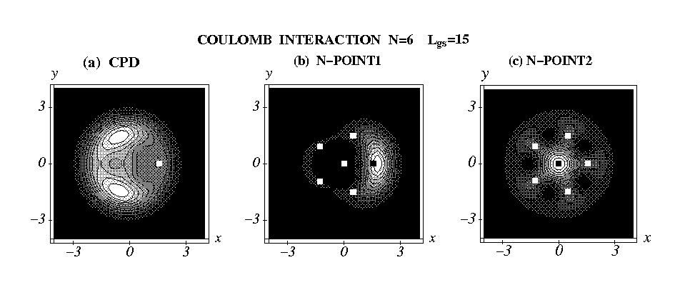
Figure 34: Contour plots of the CPD (a) and $N$-point correlation function (b) and (c) for $N=6$ bosons with $L_{\rm{gs}}=15$ interacting via a Coulomb repulsion. The white squares indicate the positions of the fixed particles. The black square in (b) and (c) indicates the position of the 6th particle according to the classical $(1,5)$ molecular configuration. Note the different arrangements of the five fixed particles, i.e., (b) one fixed particle at the center and (c) no fixed particle at the center. Note also that the CPD in (a) fails to reveal the $(1,5)$ pattern, which, however, is clearly seen in the $N$-point correlation functions in both (b) and (c). Lengths in units of $\Lambda$. The vertical scales are arbitrary, but the same in (b) and (c).

Figure 35: Contour plots of the CPD (a) and $N$-point correlation function (b) and (c) for $N=6$ bosons with $L_{\rm{gs}}=15$ interacting via a $\delta$-repulsion. The white squares indicate the positions of the fixed particles. The black square in (b) and (c) indicates the position of the 6th particle according to the classical $(1,5)$ molecular configuration. Note the different arrangements of the five fixed particles, i.e., (b) one fixed particle at the center and (c) no fixed particle at the center. Note also that the CPD in (a) fails to reveal the $(1,5)$ pattern, which, however, is clearly seen in the $N$-point correlation functions in both (b) and (c). Lengths in units of $\Lambda$. The vertical scales are arbitrary, but the same in (b) and (c).

However, for $\nu>1/2$, the azimuthal variations may not be visible in the CPDs, in spite of the characteristic step-like ground-state spectra [see figure 32 for $N=6$ bosons]. This paradox is resolved when one considers higher-order correlations, and in particular $N$-point correlations [see Equation (8.8)]. In figure 34 and figure 35, we plot the $N$-point correlation functions for $N=6$ bosons and $L_{\rm{gs}}=15$ for both the Coulomb interaction and $\delta$-repulsion, respectively, and we compare them against the corresponding CPDs. The value of 15 is divisible by 5, and one expects this state to be associated with a $(1,5)$ molecular configuration. It is apparent that the CPDs fail to portray such fivefold azimuthal pattern. The $(1,5)$ pattern, however, is clear in the $N$-point correlations (middle and right panels). One has two choices for choosing the positions of the first five particles (white dots), i.e., one choice places one white dot at the center and the other choice places all five white dots on the vertices of a regular pentagon. For both choices, as shown by the contour lines in the figures, the position of maximum probability for the sixth boson coincides with the point that completes the $(1,5)$ configuration [see the black dots in the middle and right panels].

Note that the differences in the CPDs and $N$-point correlation functions between the Coulomb and the $\delta$-repulsion are rather minimal.

9 Summary

This report reviewed the physics of strong correlations in two-dimensional small finite-size condensed-matter systems, such as electrons in quantum dots and repelling bosons in harmonic traps. It was shown that strong correlations in such systems relate to the appearance of symmetry breaking at the mean-field level of description. Particular attention was given to the similarities of symmetry breaking in these systems despite the different interparticle interactions (Coulombic repulsion in quantum dots versus a contact potential for neutral bososns in harmonic traps).

The universal aspects of symmetry breaking in small systems (including nuclei and molecules in quantum chemistry) have been exploited to develop a two-step method of symmetry breaking at the unrestricted Hartree-Fock level and subsequent symmetry restoration via post Hartree-Fock projection techniques. In conjunction with exact-diagonalization calculations, the two-step method was used to describe a vast range of strongly-correlated phenomena associated with particle localization and formation of crystalline (molecular) structures of electrons in quantum dots and bosons in harmonic traps. Due to their finite size, these crystalline structures are different from the familiar rigid crystals of extended systems; they rather resemble and exhibit similarities with the natural 3D molecules (e.g., ro-vibrational spectra).

It was shown that strongly-correlated phenomena emerging from symmetry breaking include:

(I) Chemical bonding, dissociation, and entanglement in quantum dot molecules and in electron molecular dimers formed within a single anisotropic quantum dot, with potential technological applications to solid-state quantum-computing devices.

(II) Electron crystallization, with localization on the vertices of concentric polygonal rings, and formation of rotating electron molecules in circular quantum dots. At zero magnetic field, the REMs can approach the limit of a rigid rotor; at high magnetic field, the REMs are highly floppy, with the rings rotating independently of each other.

(III) In the lowest Landau level, the rotating electron molecules are described by parameter-free analytic many-body wave functions, which are an alternative to the composite-fermion and Jastrow/Laughlin approaches, offering a new point of view of the fractional quantum Hall regime in quantum dots (with possible implications for the thermodynamic limit).

(IV) Crystalline phases of strongly repelling bosons. In the case of rotating traps and in analogy with the REMs, such repelling bosons form rotating boson molecules, which are energetically favored compared to the Gross-Pitaevkii solutions, in particular in the regime of vortex formation.

Appendix A

In this Appendix, we briefly review the single-particle wave functions and associated energy spectra of a two-dimensional circular harmonic oscillator under the influence of a perpendicular magnetic field $B$ (relevant to the case of quantum dots) or under rotation with angular frequency $\Omega$ (relevant to the case of trapped atomic gases in rotating harmonic traps). These single-particle wave functions and associated spectra are known as the Darwin-Fock states and energy levels, after the names of the authors of two original papers [162, 163] on this subject.

Figure 36: (Color online) The Darwin-Fock single-particle energy levels of a 2D harmonic oscillator under the effect of a perpendicular magnetic field $B$ as a function of $\eta=\omega_{c}/\omega_{0}$, where $\omega_{c}$ is the cyclotron frequency and $\omega_{0}$ is the frequency specifying the 2D harmonic confinement. A specific color (online) indicates orbitals with the same number of radial nodes.

A.1                Two-dimensional isotropic oscillator in a perpendicular magnetic field

In this case, the Hamiltonian (for an electron of mass $m^{*}$) is given by:

$$H=\frac{1}{2m^{*}}({\bf p}-\frac{e}{c}{\bf A})^{2}+\frac{1}{2}m^{*}\omega_{0}^{2}{\bf r}^{2},$$ (1.1)

where ${\bf r}=(x,y)$ and $\omega_{0}$ is the frequency of the oscillator. In the symmetric gauge, the vectror potential is given by ${\bf A}=({\bf B}\times{\bf r})/2$, and the Hamiltonian (1.1) can be rewritten in the form

$$H=\frac{{\bf p}^{2}}{2m^{*}}-\frac{1}{2}\omega_{c}\hat{l}+\frac{1}{2}m^{*}\tilde{\omega}^{2}{\bf r}^{2},$$ (1.2)

where $\hat{l}=-\rmi\hbar(x\partial/\partial y-y\partial/\partial x)$ is the angular momentum operator of the electron (in the $z$ direction), $\omega_{c}=eB/(m^{*}c)$ is the cyclotron frequency, and $\tilde{\omega}=\sqrt{\omega_{0}^{2}+\omega_{c}^{2}/4}$ is the effective-confinement frequency.

The eigenfunctions of the Hamiltonian (1.2) have the same functional form as those of a 2D harmonic oscillator at B=0, but with an effective frequency $\tilde{\omega}$, i.e., in polar coordinates

$$\phi_{n,l}(\rho,\theta)={\cal N}_{n,l}\rho^{|l|}\rme^{-\rho^{2}/2}\rme^{\rmi l\theta}L_{n}^{|l|}(\rho^{2}),$$ (1.3)

with $\rho=r/\tilde{l}$; the characteristic length $\tilde{l}$ is given by $\tilde{l}=\sqrt{\hbar/(m^{*}\tilde{\omega})}$. In (1.3), the index $n$ denotes the number of nodes in the radial direction, and $l$ (without any subscript or tilde) denotes the angular-momentum quantum numbers; the $L_{n}^{|l|}$’s are associated Laguerre polynomials.

The single-particle energy spectrum corresponding to the Hamiltonian (1.2) is plotted in figure 36; the associated eigenenergies are given by

$$\frac{E_{n,l}}{\hbar\omega_{0}}=(2n+|l|+1)\sqrt{1+\frac{\eta^{2}}{4}}-\frac{l}{2}\eta,$$ (1.4)

with $\eta=\omega_{c}/\omega_{0}$.

In the limit of $\omega_{c}/(2\omega_{0})\rightarrow\infty$, one can neglect the external confinement, and the energy spectrum in Equation (1.4) reduces to that of the celebrated Landau levels, i.e.,

$$E_{\cal M}=\hbar\omega_{c}({\cal M}+\frac{1}{2}),$$ (1.5)

where ${\cal M}=n+(|l|-l)/2$ is the Landau-level index.

We remark that the Landau levels are infinitely degenerate. The lowest Landau level ${\cal M}=0$ contains all nodeless levels ($n=0$) with arbitrary positive angular momentum $l\geq 0$.

Figure 37: (Color online) The Darwin-Fock single-particle energy levels of a 2D harmonic oscillator rotating with angular frequency $\Omega$ as a function of $\eta=\Omega/\omega_{0}$, where $\omega_{0}$ is the frequency specifying the 2D harmonic confinement. A specific color (online) indicates orbitals with the same number of radial nodes.

A.2               Two-dimensional rotating harmonic oscillator

In the case of a rotating isotropic oscillator, instead of the expression (1.2), one has the following single-particle Hamiltonian:

$$H=\frac{{\bf p}^{2}}{2m}-\Omega\hat{l}+\frac{1}{2}m\omega_{0}^{2}{\bf r}^{2},$$ (1.6)

where the mass of the particle (e.g., a bosonic or fermionic atom) is denoted by $m$; $\Omega$ denotes the rotational frequency.

From a comparison of the second terms in (1.2) and (1.6), one derives the correspondence $\Omega\rightarrow\omega_{c}/2$.

We note that, unlike the application of a perpendicular magnetic field, the rotation does not generate an effective confinement different from the original external one [compare the third terms between (1.2) and (1.6)]. As a result, the eigenfunctions of the Hamiltonian (1.6) are given by the expressions (1.3), but with $\rho=r/l_{0}$ where the characteristic length $l_{0}=\sqrt{\hbar/(m\omega_{0})}$.

The single-particle energy spectrum corresponding to the Hamiltonian (1.6) is plotted in figure 37 and the associated eigenenergies are given by

$$\frac{E_{n,l}}{\hbar\omega_{0}}=(2n+|l|+1)-l\eta,$$ (1.7)

with $\eta=\Omega/\omega_{0}$.

For $\Omega/\omega_{0}=1$, the energy spectrum in Equation (1.7) reduces to that of the corresponding Landau levels, i.e.,

$$E_{\cal M}=2\hbar\omega_{0}({\cal M}+\frac{1}{2}),$$ (1.8)

where ${\cal M}=n+(|l|-l)/2$ is the Landau-level index.

As was the case with the perpendicular magnetic field, the Landau levels are infinitely degenerate, and the lowest Landau level ${\cal M}=0$ contains all nodeless levels ($n=0$) with arbitrary positive angular momentum $l\geq 0$. However, unlike the magnetic-field case where $\hbar\omega_{c}$ depends on $B$, the energy gap between the Landau levels in the case of rotation is independent of $\Omega$ and equals $2\hbar\omega_{0}$.

References

- [1] Ruder H, Wunner G, Herold H and Geyer F 1994 Atoms in Strong Magnetic Fields (Berlin: Springer Verlag)
- [2] Kouwenhoven L P, Austing D G and Tarucha S 2001 Rep. Prog. Phys. 64 701
- [3] Reimann S M and Manninen M 2002 Rev. Mod. Phys. 74 1283
- [4] Dalfovo F, Giorgini S, Pitaevskii L P and Stringari S 1999 Rev. Mod. Phys. 71 463
- [5] Leggett A J 2001 Rev. Mod. Phys. 73 307
- [6] Bohigas O 1990 In Chaos and Quantum Physics edited by Giannoni M-J, Voros A and Zinn-Justin J (Amsterdam: North-Holland) p 87
- [7] Beenakker C W J 1997 Rev. Mod. Phys. 69 731
- [8] Alhassid Y 2000 Rev. Mod. Phys. 72 895
- [9] Anderson P W 1972 More Is Different: Broken symmetry and the hierarchical structure of science Science 177 393
- [10] Anderson P W 1984 Basic Notions of Condensed Matter Physics (Reading, MA: Addison-Wesley) pp 44 - 47
- [11] Bohr Å and Mottelson B R 1953 K. Danske Vidensk. Selsk. Mat.-Fys. Medd. 27 No 16
- [12] Nilsson S G 1955 K. Danske Vidensk. Selsk. Mat.-Fys. Medd. 29 No 16
- [13] Nazarewicz W 1994 Nucl. Phys. A 574 c27
- [14] Clemenger K L 1985 Phys. Rev. B 32 1359
- [15] Yannouleas C and Landman U 1995 Phys. Rev. B 51 1902
- [16] Yannouleas C, Landman U and Barnett R N 1999 In Metal Clusters edited by Ekardt W (Chichester: Wiley) p 145
- [17] Strutinsky V M 1967 Nucl. Phys. A95 420; Strutinsky V M 1968 Nucl. Phys. A122 1
- [18] Ring P and Schuck P 1980 The Nuclear Many-body Problem (New York: Springer-Verlag)
- [19] Szabo A and Ostlund N S 1989 Modern Quantum Chemistry (New York: McGraw-Hill)
- [20] Yannouleas C and Landman U 1999 Phys. Rev. Lett. 82 5325; 2000 Phys. Rev. Lett. 85 2220(E)
- [21] Yannouleas C and Landman U 2000 Phys. Rev. B 61 15895
- [22] Yannouleas C and Landman U 2001 Eur. Phys. J. D 16 373
- [23] Yannouleas C and Landman U 2002 J. Phys.: Condens. Matter 14 L591
- [24] Yannouleas C and Landman U 2002 Phys. Rev. B 66 115315
- [25] Yannouleas C and Landman U 2003 Phys. Rev. B 68 035325
- [26] Yannouleas C and Landman U 2003 Phys. Rev. B 68 035326
- [27] Müller H-M and Koonin S E 1996 Phys. Rev. B 54 14532
- [28] Wigner E P 1934 Phys. Rev. 46 1002
- [29] Hirose K and Wingreen N S 1999 Phys. Rev. B 59 4604
- [30] Peierls R E and Yoccoz J 1957 Proc. Phys. Soc. (London) A70 381
- [31] Löwdin P-O 1955 Phys. Rev. 97 1509
- [32] Löwdin P-O 1964 Rev. Mod. Phys. 36 966
- [33] Fukutome H 1981 Int. J. Quantum Chem. 20 955, and references therein
- [34] Rodriguez T R, Egido J L and Robledo L M 2005 Phys. Rev. C 72 064303
- [35] Schmid K W 2004 Prog. Part. Nucl. Phys. 52 565
- [36] Bender M, Flocard H and Heenen P H 2003 Phys. Rev. C 68 044321
- [37] Stoitsov M V, Dobaczewski J, Nazarewicz W, Pittel S and Dean D J 2003 Phys. Rev. C 68 054312
- [38] Bender M, Heenen P H and Reinhard P-G (2003) Rev. Mod. Phys. 75 121
- [39] Reinhard P-G, Nazarewicz W, Bender M and Maruhn J A 1996 Phys. Rev. C 53 2776
- [40] Fernandez M A and Egido J L 2003 Phys. Rev. B 68 184505
- [41] Ellenberger C, T. Ihn T, Yannouleas C, Landman U, Ensslin K, Driscoll D and Gossard A C 2006 Phys. Rev. Lett. 96 126806
- [42] Yannouleas C and Landman U 2006 phys. stat. sol. (a) 203 1160
- [43] Yannouleas C and Landman U 2006 Proc. Natl. Acad. Sci. USA 103 10600
- [44] Ihn T, Ellenberger C, Ensslin K, Yannouleas C, Landman U, Driscoll D C and Gossard A C 2007 Int. J. Mod. Phys. B 21 1316
- [45] Zumbühl D M, Marcus C M, Hanson M P and Gossard A C 2004 Phys. Rev. Lett. 93 256801
- [46] Yannouleas C and Landman U 2002 Int. J. Quantum Chem. 90 699
- [47] Loss D and D.P. DiVincenzo D P 1998 Phys. Rev. A 57 120
- [48] Burkard G, Loss D and DiVincenzo D P 1999 Phys. Rev. B 59 2070
- [49] Taylor J M, Engel H A, Dür W, Yacoby A, Marcus C M, Zoller P and Lukin M D 2005 Nature Phys. 1 177
- [50] Yannouleas C and Landman U 2000 Phys. Rev. Lett. 85 1726
- [51] Yannouleas C and Landman U 2004 Phys. Rev. B 69 113306
- [52] Yannouleas C and Landman U 2004 Phys. Rev. B 70 235319
- [53] Li Y S, Yannouleas C and Landman U 2006 Phys. Rev. B 73 075301
- [54] Leggett T 2004 Science 305 1921
- [55] Laughlin R B 1983 Phys. Rev. Lett. 50 1395
- [56] Jain J K 1989 Phys. Rev. Lett. 63 199
- [57] Jain J K 1990 Phys. Rev. B 41 7653
- [58] Yoshioka D 2002 The Quantum Hall Effect (Berlin: Springer)
- [59] Jain J K 2007 Composite Fermions (New York: Cambridge University Press)
- [60] Romanovsky I, Yannouleas C and Landman U 2004 Phys. Rev. Lett. 93 230405
- [61] Tonks L 1936 Phys. Rev. 50 955
- [62] Girardeau M 1960 J. Math. Phys. (N.Y.) 1 516
- [63] Romanovsky I, Yannouleas C, Baksmaty L O and Landman U 2006 Phys. Rev. Lett. 97 090401
- [64] Laughlin R B 1999 Rev. Mod. Phys. 71 863
- [65] Landman U 2005 Proc. Natl. Acad. Sci. USA 102 6671
- [66] Löwdin P-O 1959 Adv. Chem. Phys. vol II p 207
- [67] Wilkin N K and Gunn J M F 2000 Phys. Rev. Lett. 84 6
- [68] Viefers S, Hansson T H and Reimann S M 2000 Phys. Rev. A 62 053604
- [69] Cooper N R, Wilkin N K and Gunn J M F 2001 Phys. Rev. Lett. 87 120405
- [70] Regnault N and Jolicoeur Th 2003 Phys. Rev. Lett. 91 030402
- [71] Chang C-C, Regnault N, Jolicoeur Th and Jain J K 2005 Phys. Rev. A 72 013611
- [72] Baksmaty L O, Yannouleas C and Landman U 2007 Phys. Rev. A 75 023620
- [73] Tarucha S, Austing D G, Honda T, van der Hage R J, Kouwenhoven L P 1996 Phys. Rev. Lett. 77 3613
- [74] Nishi Y, Maksym P A, Austing D G, Hatano T, Kouwenhoven L P, Aoki H, Tarucha S 2006 Phys. Rev. B 74 033306
- [75] Nishi Y, Tokura Y, Gupta J, Austing G and Tarucha S 2007 Phys. Rev. B 75 121301
- [76] De Giovannini U, Cavaliere F, Cenni R, Sassetti M and Kramer B 2007 New J. Phys. 9 93
- [77] Rontani M, Cavazzoni C, Bellucci D and Goldoni G 2006 J. Chem. Phys. 124 124102
- [78] Ghosal A, Güçlü A D, Umrigar C J, Ullmo D and Baranger H U 2006 Nature Phys. 2 336
- [79] Ciorga M, Sachrajda A S, Hawrylak P, Gould C, Zawadzki P, Jullian S, Feng Y and Wasilewski Z 2000 Phys. Rev. B 61 R16315
- [80] Kyriakidis J, Pioro-Ladriere M, Ciorga M, Sachrajda A S and Hawrylak P 2002 Phys. Rev. B 66 035320
- [81] Hatano T, Stopa M and Tarucha S 2005 Science 309 268
- [82] Heitler H and London F 1927 Z. Phys. 44 455
- [83] Avinun-Kalish M, Heiblum M, Zarchin O, Mahalu D and Umansky V 2005 Nature 436 529
- [84] Gurvitz S A 2007 arXiv:0704.1260v1
- [85] Kinoshita G T, Wenger T and and Weiss D S 2004 Science 305 1125
- [86] Paredes B, Widera A, Murg V, Mandel O, Folling S, Cirac I, Shlyapnikov G V, Hansch T W and Bloch I 2004 Nature (London) 429 277
- [87] Greiner M, Mandel O, Esslinger T, Hansch T W and Bloch I 2002 Nature (London) 415 39
- [88] Mueller E J, Ho T L, Ueda M and Baym G 2006 Phys. Rev. A 74 033612
- [89] Zhang L-X, Melnikov D V and Leburton J-P 2006 Phys. Rev. B 74 205306
- [90] Hallam L D, Weis J and Maksym P A 1996 Phys. Rev. B 53 1452
- [91] Koskinen M, Manninen M and Reimann S M 1997 Phys. Rev. Lett. 79 1389
- [92] Lee I H, Rao V, Martin R M and Leburton J-P 1998 Phys. Rev. B 57 9035
- [93] Barnett R N, Cleveland C L, Hakkinen H, Luedtke W D, Yannouleas C and Landman U 1999 Eur. Phys. J. D 9 95
- [94] Matagne P, Leburton J-P, Austing D G and Tarucha S 2002 Phys. Rev. B 65 085325
- [95] Saarikoski H, Harju A, Puska M J and Nieminen R M 2004 Phys. Rev. Lett. bf 93 116802
- [96] Borgh M, Toreblad M, Koskinen M, Manninen M, Åberg S and Reimann S M 2005 Int. J. Quantum Chem. 105 817
- [97] Pfannkuche D, Gudmundsson V and Maksym P A 1993 Phys. Rev. B 47 2244
- [98] Fujito M, Natori A and Yasunaga H 1996 Phys. Rev. B 53 9952
- [99] Bednarek S, Szafran B and Adamowski J 1999 Phys. Rev. B 59 013036
- [100] Rontani M, Rossi F, Manghi F and Molinari E 1999 Phys. Rev. B 59 010165
- [101] Reusch B, Häusler W and Grabert H 2001 Phys. Rev. B 63 113313
- [102] Szafran B, Bednarek S and Adamowski J 2003 Phys. Rev. B 67 045311
- [103] Szafran B, Bednarek S, Adamowski J, Tavernier M B, Anisimovas E and Peeters F M 2004 Eur. Phys. J. D 28 373
- [104] Emperador A, Lipparini E and Serra L 2006 Phys. Rev. B 73 235341
- [105] Lipparini E 2003 Modern Many-Particle Physics: Atomic Gases, Quantum Dots and Quantum Fluids (London: World Scientific)
- [106] Pople J A and Nesbet R K 1954 J. Chem. Phys. 22 571
- [107] Overhauser A W 1960 Phys. Rev. Lett. 4 415
- [108] Thouless D J 1961 The Quantum Mechanics of Many-Body Systems (New York: Academic Press)
- [109] Adams W H 1962 Phys. Rev. 127 1650
- [110] Čížek J and Paldus J 1967 J. Chem. Phys. 47 3976
- [111] Carbó R and Klobukowski M 1990 Self-Consistent Field: Theory and Applications (Amsterdam: Elsevier Science Publishers)
- [112] Lozovik Yu E 1987 Usp. Fiz. Nauk 153 356 [1987 Sov. Phys. Usp. 30 912]
- [113] Bedanov V M and Peeters F M 1994 Phys. Rev. B 49 2667
- [114] Kong M, Partoens B and Peeters F M 2002 Phys. Rev. E 65 046602
- [115] Overhauser A W 1962 Phys. Rev. 128 1437
- [116] Wigner E P 1959 Group Theory and its Application to the Quantum Mechanics of Atomic Spectra (New York: Academic Press)
- [117] Hashimoto K 1982 Int. J. Quantum Chem. 22 397
- [118] Igawa A 1995 Int. J. Quantum Chem. 54 235
- [119] Pauncz R 2000 The Construction of Spin Eigenfunctions: An Exercise Book (New York: Kluwer/Plenum)
- [120] Goddard W A III, Dunning T H Jr, Hunt W J and Hay P J 1973 Accounts Chem. Res. 6 368
- [121] Gerratt J and Lipscomb W N 1968 Proc. Natl. Acad. Sci. USA 59 332
- [122] De Giovannini U, Cavaliere F, Cenni R, Sassetti M and Kramer B 2007 arXiv:0707.3705v1
- [123] Zduńczuk H, Dobaczewski J and Satuła W 2007 Int. J. Mod. Phys. E 16 377
- [124] Kamlah A 1968 Z. Phys. 216 52
- [125] Yoshioka D J and Lee P A 1983 Phys. Rev. B 27 4986
- [126] MacDonald A H, Yang S R E and Johnson M D 1993 Aust. J. Phys. 46 345
- [127] Ruan W Y, Liu Y Y, Bao C G and Zhang Z Q 1995 Phys. Rev. B 51 7942
- [128] Maksym P A 1996 Phys. Rev. B 53 10871
- [129] Girvin S M and Jach T 1983 Phys. Rev. B 28 4506
- [130] Maksym P A and Chakraborty T 1990 Phys. Rev. Lett. 65 108
- [131] Seki T, Kuramoto Y and Nishino T 1996 J. Phys. Soc. Jpn. 65 3945
- [132] Maksym P A, Imamura H, Mallon G P and Aoki H 2000 J. Phys.: Conden. Matter 12 R299
- [133] Jacak L, Hawrylak P and Wojs A 1998 Quantum Dots (Berlin: Springer), and references therein.
- [134] Melnikov D V, Matagne P, Leburton J-P, Austing D G, Yu G, Tarucha S, Fettig J and Sobh N 2005 Phys. Rev. B 72 085331
- [135] Melnikov D V and Leburton J-P 2006 Phys. Rev. B 73 155301
- [136] Perdew J P, Savin A and Burke K 1995 Phys. Rev. A 51 4531
- [137] Savin A 1996 In Recent Developments and Applications of Modern Density Functional Theory edited by Seminario J M (Amsterdam: Elsevier) p 327
- [138] Bauernschmitt R and Ahlrichs R J 1996 Chem. Phys. 104 9047
- [139] Abedinpour S H, Polini M, Xianlong G and Tosi M P 2007 Eur. Phys. J. B 56 127
- [140] Laegsgaard J and Stokbro K 2001 Phys. Rev. Lett. 86 2834
- [141] Savrasov S Y, Kotliar G and Abrahams E 2001 Nature (London) 410 793
- [142] Adamo C, Barone V, Bencini A, Broer R, Filatov M, Harrison N M, Illas F, Malrieu J P and Moreira I D R 2006 J. Chem. Phys. 124 107101
- [143] Rong C, Lian S, Yin D, Shen B, Zhong A, Bartolotti L and Liu S 2006 J. Chem. Phys. 125 174102
- [144] Illas F, Moreira I D R, Bofill J M and Filatov M 2006 Theor. Chem. Acc. 116 587
- [145] Thouless D J and Valatin J G 1962 Nucl. Phys. 31 211
- [146] Bertsch G F and Hagino K 2001 Yad. Fiz. 64 646 [2001 Phys. Part. Nucl. 64 588]
- [147] Nazmitdinov R G, Almehed D and Dönau F 2002 Phys. Rev. C 65 041307
- [148] Serra Ll, Nazmitdinov R G and Puente A 2003 Phys. Rev. B 68 035341
- [149] Hill D L and Wheeler J A 1953 Phys. Rev. 89 1102
- [150] Griffin J J and Wheeler J A 1957 Phys. Rev. 108 311
- [151] Öhberg P and Stenholm S 1998 Phys. Rev. A 57 1272
- [152] Esry B D and Greene C H 1999 Phys. Rev. A 59 1457
- [153] Alon O E, Streltsov A I and Cederbaum L S 2005 Phys. Rev. Lett. 95 030405
- [154] Esry B D 1997 Phys. Rev. A 55 1147
- [155] Romanovsky I A 2006 Ph. D. Thesis, Georgia Institute of Technology, Atlanta, http://etd.gatech.edu/theses/available/etd-07102006-041659.
- [156] Cederbaum L S and Streltsov A I 2003 Phys. Lett. A 318 564
- [157] Hurley A C 1976 Introduction to the Electron Theory of Small Molecules (London: Academic Press)
- [158] Tsiper E V 2002 J. Math. Phys. 43 1664
- [159] Bertsch G F and Papenbrock T 1999 Phys. Rev. Lett. 83 5412
- [160] Lehoucq R B, Sorensen D C and Yang C 1998 ARPACK Users’ Guide: Solution of Large-Scale Eigenvalue Problems with Implicitly Restarted Arnoldi Methods (Philadelphia: SIAM)
- [161] Tsiper E V and Goldman V J 2001 Phys. Rev. B 64 165311
- [162] Darwin C G 1930 Proc. Cambridge Philos. Soc. 27 86
- [163] Fock V 1928 Z. Phys. 47 446
- [164] Anisimovas E and Matulis A 1998 J. Phys.: Condens. Matter 10 601
- [165] Eto M 1997 Jpn. J. Appl. Phys. 36 3924
- [166] Hawrylak P and Pfannkuche D 1993 Phys. Rev. Lett. 70 485
- [167] Mikhailov S A 2002 Phys. Rev. B 65 115312
- [168] Mikhailov S A and Savostianova N A 2002 Phys. Rev. B 66 033307
- [169] Tavernier M B, Anisimovas E, Peeters F M, Szafran B, Adamowski J and Bednarek S 2003 Phys. Rev. B 68 205305
- [170] Wensauer A, Korkusinski M and Hawrylak P 2004 Solid State Commun. 130 115
- [171] Ruan W Y and Cheung H-F 1999 J. Phys.: Condens. Matter 11 435
- [172] Creffield C E, Hausler W, Jefferson J H and Sarkar S 1999 Phys. Rev. B 59 10719
- [173] Laughlin R B 1983 Phys. Rev. B 27 3383
- [174] Kawamura T and Jain J K 1996 J. Phys.: Condens. Matter 8 2095
- [175] Reimann S M, Koskinen M and Manninen M 2000 Phys. Rev. B 62 8108
- [176] Jeon G S, Chang C-C and Jain J K 2007 Eur. Phys. J. B 55 271
- [177] Barberan N, Lewenstein M, Osterloh K and Dagnino D 2006 Phys. Rev. A 73 063623
- [178] Reimann S M, Koskinen M, Yu Y and Manninen M 2006 New J. Phys. 8 59
- [179] Wagner M, Merkt U and Chaplik A V 1992 Phys. Rev. B 45 R1951
- [180] Drouvelis P S, Schmelcher P and Diakonos F K 2004 Phys. Rev. B 69 035333
- [181] Harju A, Siljamäki S and Nieminen R M 2002 Phys. Rev. Lett. 88 226804
- [182] Klironomos A D, Meyer J S and Matveev K A 2006 Europhys. Lett. 74 679
- [183] Piacente G, Schweigert I V, Betouras J J and Peeters F M 2004 Phys. Rev. B 69 045324
- [184] Li Y, Yannouleas C and Landman U 2007 to be published
- [185] Dür W, Vidal G and Cirac J I 2000 Phys. Rev. A 62 062314
- [186] Coffman V, Kundu J and Wootters W K 2000 Phys. Rev. A 61 052306
- [187] Ohno K, Esfarjani K and Kawazoe Y 1999 Computational Materials Science: From Ab Initio to Monte Carlo Methods (New York: Springer)
- [188] Egger R, Häusler W, Mak C H and Grabert H 1999 Phys. Rev. Lett. 82 3320; 1999 Phys. Rev. Lett. 83 462(E)
- [189] Filinov A V, Lozovik Yu E and Bonitz M 2000 Phys. Status Solidi B 221 231
- [190] Harting J, Mülken and Borrmann P 2000 Phys. Rev. B 62 10207
- [191] Reusch B and Egger R 2003 Europhys. Lett. 64 84
- [192] Weiss S and Egger R 2005 Phys. Rev. B 72 245301
- [193] Tanatar B and Ceperley D M 1989 Phys. Rev. B 39 5005
- [194] Pederiva F, Umrigar C J and Lipparini E 2000 Phys. Rev. B 62 8120
- [195] Harju A, Siljamäki S and Nieminen R M 2002 Phys. Rev. B 65 075309
- [196] Güçlü A D and Umrigar C J 2005 Phys. Rev. B 72 045309
- [197] Ghosal A, Güçlü A D, Umrigar C J, Ullmo D and Baranger H U 2007 arXiv:cond-mat/0702666v1
- [198] Mora Ch and Waintal X 2007 Phys. Rev. Lett. 99 030403
- [199] Salis G, Kato Y, Ensslin K, Driscoll D C, Gossard A C and Awschalom D D 2001 Nature 414 619
- [200] Paskauskas R and You L 2001 Phys. Rev. A 64 042310
- [201] Schliemann J, Cirac J, Kus M, Lewenstein M and Loss D 2001 Phys. Rev. A 64 022303
- [202] Kellman M E and Herrick D R 1980 Phys. Rev. A 22 1536
- [203] Kellman M E 1997 Int. J. Quantum Chem. 65 399
- [204] Berry R S 1989 Contemp. Phys. 30 1
- [205] Sommerfeld A 1923 Rev. Sci. Inst. 7 509
- [206] Pais A 1991 Niels-Bohr’s Times (Oxford: Clarendon)
- [207] Van Vleck J H 1922 Phil. Mag. 44 842
- [208] Born M 1927 The Mechanics of the Atom (New York: Ungar)
- [209] Leopold J G and Percival I C 1980 J. Phys. B 13 1037
- [210] Wintgen D, Richter K and Tanner G 1992 Chaos 2 19
- [211] Ezra G S and Berry R S 1983 Phys. Rev. A 28 1974
- [212] Watanabe S and Lin C D 1986 Phys. Rev. A 34 823
- [213] Creffield C E, Häusler W, Jefferson J H and Sarkar S 1999 Phys. Rev. B 59 10719
- [214] Häusler W, Reusch B, Egger R and Grabert H 2000 Physica B 284 1772
- [215] Matulis A and Peeters F M 2001 Solid State Commun. 117 655
- [216] Filinov A V, Bonitz M and Lozovik Yu E 2001 Phys. Rev. Lett. 86 3851
- [217] Sundqvist P A, Volkov S Y, Lozovik Yu E and Willander M 2002 Phys. Rev. B 66 075335
- [218] Mikhailov S A and Ziegler K 2002 Eur. Phys. J. B 28 117
- [219] Mikhailov S A 2002 Physica E 12 884
- [220] Creffield C E, Jefferson J H, Sarkar S and Tipton D L J 2000 Phys. Rev. B 62 7249
- [221] Rontani M, Goldoni G, Manghi F and Molinari E 2002 Europhys. Lett. 58 555
- [222] Bolton F and Rössler U Superlatt. Microstruct. 13 139
- [223] Jain J K and Kamilla R K 1997 Int. J. Mod. Phys. B 11 2621
- [224] Goldmann E and Renn S R 1997 Phys. Rev. B 56 13296
- [225] Eric Yang S-R and Han J H 1998 Phys. Rev. B 57 R12681
- [226] Taut M 2000 J. Phys.: Condens. Matter 12 3689
- [227] Manninen M, Viefers S, Koskinen M and Reimann S M 2001 Phys. Rev. B 64 245322
- [228] Wan X, Yang K and Rezayi E H 2002 Phys. Rev. Lett. 88 056802
- [229] Jain J K and Kawamura T 1995 Europhys. Lett. 29 321
- [230] Maki K and Zotos X 1983 Phys. Rev. B 28 4349
- [231] Wunsch B, Stauber T and Guinea F 2007 arXiv:0707.2948v2
- [232] Dai Z, Zhu J-L, Yang N and Wang Y 2007 arXiv:cond-mat/0702256v2
- [233] Shi C, Jeon G S and Jain J K 2007 Phys. Rev. B 75 165302
- [234] Jeon G S, Chang C-C and Jain J K 2004 J. Phys.: Condens. Matter 16 L271
- [235] Chang C-C, Jeon G S and Jain J K 2005 Phys. Rev. Lett. 94 016809
- [236] Laughlin R B 1987 In The Quantum Hall Effect Edited by Prange R E and Girvin S M (New York: Springer) p 233
- [237] Jeon G S, Chang C-C and Jain J K 2004 Phys. Rev. B 69 R241304
- [238] Lam P K and Girvin S M 1984 Phys. Rev. B 30 473
- [239] Tavernier M B, Anisimovas E and Peeters F M 2004 Phys. Rev. B 70 155321
- [240] Yang S R E, MacDonald A H and Johnson M D 1993 Phys. Rev. Lett. 71 3194
- [241] Löwdin P-O 1962 Rev. Mod. Phys. 34 520
- [242] Toreblad M, Borgh M, Koskinen M, Manninen M and Reimann S M 2004 Phys. Rev. Lett. 93 090407
- [243] Toreblad M, Yu Y, Reimann S M, Koskinen M and Manninen M 2006 J. Phys. B 39 2721
- [244] Pan W, Stormer H L, Tsui D C, Pfeiffer L N, Baldwin K W and West K W 2002 Phys. Rev. Lett. 88 176802
- [245] Pfeiffer L and West K W 2003 Physica E 20 57
- [246] Cornish S L, Claussen N R, Roberts J L, Cornell E A and Wieman C E 2000 Phys. Rev. Lett. 85 1795
- [247] Girardeau M D and Wright E M 2002 Laser Physics 12 8
- [248] Dunjko V, Lorent V and Olshanii M 2001 Phys. Rev. Lett. 86 5413
- [249] Kartsev P F 2003 Phys. Rev. A 68 063613
- [250] Butts R A and Rokhsar D S 1999 Nature (London) 397 327
- [251] Schellekens M, Hoppeler R, Perrin A, Gomes J V, Boiron D, Aspect A and Westbrook C I 2005 Science 310 648
- [252] Ho T L 2001 Phys. Rev. Lett. 87 060403
- [253] Fetter A L 2001 Phys. Rev. A 64 063608
- [254] Pethick C J and Smith H 2002 Bose-Einstein Condensation in Dilute Gases (Cambridge: Cambridge University Press)
- [255] Pitaevskii L P and Stringari S 2003 Bose-Einstein Condensation (Oxford: Oxford University Press)
- [256] Watanabe G, Baym G and Pethick C J 2004 Phys. Rev. Lett. 93 190401
- [257] Baym G 2005 J. Low Temp. Phys. 138 601
- [258] Madison K W, Chevy F, Wohlleben W and Dalibard J 2000 Phys. Rev. Lett. 84 806
- [259] Raman C, Abo-Shaeer J R, Vogels J M, Xu K and Ketterle W 2001 Phys. Rev. Lett. 87 210402
- [260] Engels P, Coddington I, Haljan P C and Cornell E A 2002 Phys. Rev. Lett. 89 100403
- [261] Griesmaier A, Werner J, Hensler S, Stuhler J and Pfau T 2005 Phys. Rev. Lett. 94 160401
- [262] Baranov M, Dobrek Ł, Góral K, Santos L and Lewenstein M 2002 Physica Scripta 102 74
- [263] Altman E, Demler E and Lukin M D 2004 Phys. Rev. A 70 013603
- [264] Fölling S, Gerber F, Widera A, Mandel O, Gericke T and Bloch I 2005 Nature (London) 434 481