Distributions of individual Dirac eigenvalues
for QCD at non-zero chemical potential:
RMT predictions and lattice results

Abstract:

For QCD at non-zero chemical potential $\mu$, the Dirac eigenvalues are scattered in the complex plane. We define a notion of ordering for individual eigenvalues in this case and derive the distributions of individual eigenvalues from random matrix theory (RMT). We distinguish two cases depending on the parameter $\alpha=\mu^{2}F^{2}V$, where $V$ is the volume and $F$ is the familiar low-energy constant of chiral perturbation theory. For small $\alpha$, we use a Fredholm determinant expansion and observe that already the first few terms give an excellent approximation. For large $\alpha$, all spectral correlations are rotationally invariant, and exact results can be derived. We compare the RMT predictions to lattice data and in both cases find excellent agreement in the topological sectors $\nu=0,1,2$.

1 Introduction

Studies of the properties of the Dirac operator spectrum in gauge theories, including QCD, have a long history. For example, the low-lying Dirac modes provide information about spontaneous chiral symmetry breaking through the Banks-Casher relation. The Dirac operator spectrum is also a natural object to study in lattice QCD. In the deep infrared, QCD in the $\epsilon$-regime can be described by the chiral random matrix theory (RMT) introduced in Ref. [1]. One of the advantages of RMT is that many exact analytical results can be derived. These results contain the low-energy constant (LEC) $\Sigma$ of chiral perturbation theory (chPT), and in some cases also the LEC $F$. These LECs can then be determined by fitting lattice data to the RMT curves.

The observables that are most natural to compute in RMT are the spectral density correlation functions. At zero chemical potential $\mu$, all of them are known in RMT [1, 2]. On the other hand, one can consider individual Dirac eigenvalue distributions (IED). From the lattice QCD point of view, these are the most natural observables to measure directly. Certain quantities such as the average positions of the eigenvalues are more pronounced in IEDs and therefore require less statistics to be measured reliably.

At $\mu=0$, the Dirac operator is anti-Hermitian and has a purely imaginary spectrum. In this case, all IEDs are known analytically in RMT [3]. They have become a standard tool in lattice QCD to extract $\Sigma$ in sectors of fixed topology. At $\mu\neq 0$, the Dirac operator is no longer anti-Hermitian, and its eigenvalues are scattered in the complex plane. Our work is based on an RMT for $\mu\neq 0$ [4] which has an eigenvalue representation and for which all complex density correlations (both quenched and unquenched) have been calculated. The same results can be obtained from the RMT for $\mu\neq 0$ introduced earlier by Stephanov [5] or from chPT in the $\epsilon$-regime [6, 7] and are universal in that sense. These results have been compared to data from quenched lattice simulations with staggered [8] and overlap [9] fermions at $\mu\neq 0$. A virtue of $\mu\neq 0$ is that it couples to $F$ in leading order of chPT [10] so that a comparison with lattice data allows us to extract $F$ [8].

For the IEDs at $\mu\neq 0$ much less is known. One of the problems here is to define an ordering of complex eigenvalues. Previous work on the repulsion between complex eigenvalues in RMT [11] and on the lattice [12] was done in the bulk of the spectrum, where no link to chPT is apparent. In the present work, we are interested in IEDs for eigenvalues close to the origin since they provide information on topological properties and LECs.

We first define the general notion of IEDs for complex eigenvalues, and then compute the first few IEDs approximately by truncating a so-called Fredholm determinant expansion to the first few terms. It was already observed in Ref. [13] for $\mu=0$ that this is a very good approximation. For large values of the parameter $\alpha=\mu^{2}F^{2}V$, where $V$ is the volume, we are able to derive all IEDs in closed form [14]. We use these exact results as a consistency check of the Fredholm determinant expansion. Our results are then compared to the lattice data of Ref. [9], in which the overlap Dirac operator for $\mu\neq 0$ was constructed. This operator has good chiral properties (it satisfies a Ginsparg-Wilson relation, has an exact lattice chiral symmetry and exact zero modes, and satisfies the index theorem), which is essential for the present work. The same operator is obtained if a chemical potential is introduced in the domain-wall fermion formalism in the limit of infinite extent of the fifth dimension [15]. Due to the sign problem at $\mu\neq 0$, the lattice analysis in Ref. [9] was restricted to the quenched case, and this restriction on the lattice data applies to this work as well.

2 Individual eigenvalue distributions for complex eigenvalues

Consider an operator with a finite number $N$ of complex eigenvalues, distributed according to a joint probability distribution ${\cal{P}}(\{z\})$ which is symmetric in all its arguments. We also assume a $z\to-z$ symmetry and only consider the upper half-plane ${\mathbb{C}}_{+}$. The partition function is then given by $Z=\int_{{\mathbb{C}}_{+}}\prod_{j=1}^{N}d^{2}z_{j}{\cal{P}}(\{z\})$, and the spectral density correlation functions are defined as

$$R_{k}(z_{1},...,z_{k})=\frac{1}{Z}\frac{N!}{(N-k)!}\int_{{\mathbb{C}}_{+}}d^{2}z_{k+1}\ldots d^{2}z_{N}\,{\cal{P}}_{N}(z_{1},...,z_{N})\>.$$ (1)

Now consider any one-parameter family of mutually non-intersecting closed contours $\partial J[\eta]$ which cover ${\mathbb{C}}_{+}$. For fixed $\eta$, $\partial J[\eta]$ is the boundary of a set $J[\eta]$. Let us parametrize the contour as $\partial J(z(\tau))$ with $z(\tau)\equiv x(\tau)+iy(\tau)$. We then define the $k$-th eigenvalue distribution $p_{k}(J,\tau)$ as the probability that $k-1$ eigenvalues are inside $J$, one is at the point $z(\tau)$ on the boundary $\partial J$, and the remaining $N-k$ are in the complement $\bar{J}$,

$$p_{k}(J,\tau)\equiv\frac{k}{Z}\binom{N}{k}\prod_{j=1}^{k-1}\int_{J}d^{2}z_{j}\prod_{i=k+1}^{N}\int_{\bar{J}}d^{2}z_{i}\,{\cal P}(\{z\})\big{|}_{z_{k}=z(\tau)}\>.$$ (2)

Note that the eigenvalue ordering is induced by the entire contour family. The $\{\eta,\tau\}$ play the role of generalized polar coordinates. In the following, the argument $J$ of $p_{k}$ will be suppressed. It is possible [14] to express all $p_{k}(\tau)$ through the densities Eq. (1). In particular, for the distribution of the first eigenvalue one obtains

$$p_{1}(\tau)=R_{1}(z(\tau))-\int_{J}d^{2}z_{1}\,R_{2}(z_{1},z(\tau))+\frac{(-1)^{2}}{2!}\int_{J}d^{2}z_{1}\int_{J}d^{2}z_{2}\,R_{3}(z_{1},z_{2},z(\tau))+\ldots$$ (3)

One can show that the integrated distributions $P_{k}(\eta)\equiv\int d\tau\,j(\eta,\tau)p_{k}(\eta,\tau)$ are normalized as $\int_{\eta_{\text{min}}}^{\eta_{\text{max}}}P_{k}(\eta)d\eta=1$, where $[\eta_{\text{min}},{\eta_{\text{max}}}]$ is the range of $\eta$, and $j(\eta,\tau)=|(\partial x,\partial y)/(\partial\eta,\partial\tau)|$ is the Jacobian of the transformation from $(x,y)$ to $(\eta,\tau)$. The proof is similar to that for real eigenvalues [13]. We emphasize that in this framework the choice of the contour family becomes part of the definition of the quantities we measure (i.e., the $p_{k}$’s). Different contour families in general lead to different $p_{k}$’s. However, one relation always holds trivially, namely $\sum_{k=1}^{N}p_{k}(z)=R_{1}(z)$.

3 RMT predictions

The partition function of the matrix model we use [4] reads

$$Z_{\nu}=\int dAdB\,\exp\{-N\operatorname{tr}(AA^{\dagger}+BB^{\dagger})\}\prod_{f=1}^{N_{f}}\det\left(\begin{array}[]{cc}m_{f}&iA+\hat{\mu}B\\ iA^{\dagger}+\hat{\mu}B^{\dagger}&m_{f}\end{array}\right).$$ (4)

Here, $A$ and $B$ are complex $(N+\nu)\times N$ matrices with no further symmetries, $\nu\geq 0$ is the topological charge, the $m_{f}$ are the masses of $N_{f}$ flavors of dynamical quarks, and $\hat{\mu}$ is the chemical potential in the matrix model. In the large-$N$ limit this model describes QCD in the $\epsilon$-regime. All density correlation functions of this model follow from the kernel $K_{N}(z_{i},z^{*}_{j})$ of bi-orthogonal polynomials with respect to the weight

$$w^{(N_{f},\nu)}(z_{j})=\prod_{f=1}^{N_{f}}m_{f}^{\nu}(m_{f}^{2}-z_{j}^{2})|z_{j}|^{2\nu+2}K_{\nu}\left(\frac{N(1+{\hat{\mu}}^{2})}{2{\hat{\mu}}^{2}}|z_{j}|^{2}\right)e^{\frac{N({\hat{\mu}}^{2}-1)}{4{\hat{\mu}}^{2}}\left(z_{j}^{2}+z_{j}^{*\,2}\right)}\>,$$ (5)

where $K_{\nu}$ (and $I_{\nu}$ below) are modified Bessel functions, according to

$$R_{k}(z_{1},\ldots,z_{k})=\prod_{\ell=1}^{k}w^{(N_{f},\nu)}(z_{\ell})\det_{1\leq i,j\leq k}K_{N}(z_{i},z^{*}_{j})=:\det_{1\leq i,j\leq k}\mathcal{K}_{N}(z_{i},z^{*}_{j})\>.$$ (6)

We rescale the parameters of the model such that the parameters $\alpha\equiv 2N\hat{\mu}^{2}\,(=VF^{2}\mu^{2})$, $\eta_{f}\equiv Nm_{f}\,(=V\Sigma m_{f})$, and $\xi_{k}\equiv Nz_{k}\,(=V\Sigma z_{k})$ stay finite in the large-$N$ limit. The scaling of these parameters in terms of the LECs of chPT is given in parentheses. In the quenched case, the microscopic kernel ${\cal K}_{s}(z_{i},z_{j}^{*})=\lim_{N\to\infty}{\cal K}_{N}(z_{i}/N,z_{j}^{*}/N)/N$ is given by [4]

$${\cal{K}}_{s}(z_{i},z_{j}^{*})=\frac{|z_{i}z_{j}^{*}|^{\nu+1}}{2\pi\alpha(z_{i}z_{j}^{*})^{\nu}}\sqrt{K_{\nu}\left(\frac{|z_{i}|^{2}}{4\alpha}\right)K_{\nu}\left(\frac{|z_{j}^{*}|^{2}}{4\alpha}\right)}e^{-\frac{\operatorname{Re}(z_{i}^{2}+{z_{j}^{*}}^{2})}{8\alpha}}\int_{0}^{1}dt\,e^{-2\alpha t}I_{\nu}(z_{i}\sqrt{t})I_{\nu}(z_{j}^{*}\sqrt{t})\>,$$ (7)

and the microscopic spectral density follows as $\rho_{1}(\xi)={\cal{K}}_{s}(\xi,\xi^{*})$.

Approximate computations for arbitrary $\alpha$

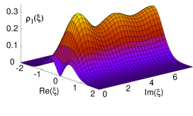
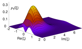
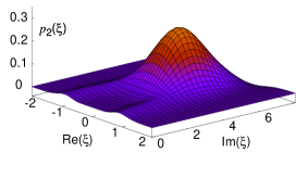
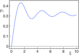
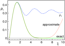
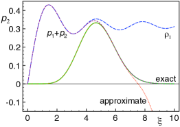
Figure 1: Top: Microscopic density $\rho_{1}(\xi)$ (left) and distributions $p_{1}(\xi)$ (middle) and $p_{2}(\xi)$ (right) of the first and second eigenvalue for an elliptic family of $\partial J[\eta]$ parametrized as $(\operatorname{Re}\xi/5)^{2}+(\operatorname{Im}\xi)^{2}=\eta^{2}$ on $\mathbb{C}_{+}$, all for $\nu=0$ and $\alpha=0.174$. Bottom: Counterparts for $\mu=0$. Left: Density. Middle: Density (dashed/blue), exact $p_{1}(\xi)$ (solid/green), and approximate $p_{1}(\xi)$ (dotted/red). Right: Density (long dashes/blue), exact $p_{1}(\xi)+p_{2}(\xi)$ (short dashes/purple), exact $p_{2}(\xi)$ (solid/green), and approximate $p_{2}(\xi)$ (dotted/red). The deviations of the approximate $p_{1}$ and $p_{2}$ from the exact results are an artifact of the truncation of the Fredholm determinant expansion.

In order to obtain the distribution $p_{1}$, we use Eq. (3) and substitute the densities from Eqs. (6) and (7). Similar formulas can be written down for other $p_{k}$’s. For practical purposes, we truncate the (so-called Fredholm determinant) expansion in Eq. (3) to the first three terms and the corresponding expansion for $p_{2}$ to the first two terms. The density $\rho_{1}(\xi)$ and the distributions $p_{1}(\xi)$ and $p_{2}(\xi)$ of the first and second eigenvalue are shown in Fig. 1, together with their counterparts in the $\mu=0$ case. For $\mu=0$ exact results are available [3] which facilitate a detailed comparison. As for $\mu=0$ [13], we see that the expansion converges rapidly. Higher-order terms merely assure that $p_{k}(\xi)$ remains zero for large $|\xi|$.

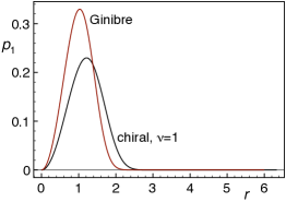
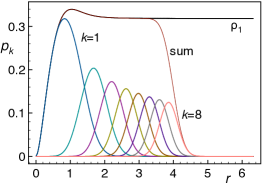
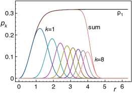
Figure 2: Left: First eigenvalue distribution as a function of the radius, for the Ginibre ensemble and for the $\nu=1$ chiral ensemble in the $\alpha\to\infty$ limit from Eq. (9). The $\nu=1$ sector was chosen since for the comparison we need exactly one eigenvalue at the origin in both cases. Middle: Spectral density Eq. (8) and distributions of the first eight eigenvalues from Eq. (9) (and similar for $p_{k}(r)$ with $k\geq 2$) as well as their sum, all in the $\alpha\to\infty$ limit and for $\nu=0$. Right: Same for $\nu=1$.

Exact results in the large-$\alpha$ limit

In the $\alpha\to\infty$ limit, the problem becomes radially symmetric. For finite but large $\alpha$, the symmetry is apparent close to the origin. The limiting microscopic spectral density expressed in the new variable $\hat{\xi}\equiv\xi/2\sqrt{\alpha}$ reads

$$\lim_{\alpha\to\infty}\rho_{1}(\hat{\xi})=\frac{2|\hat{\xi}|^{2}}{\pi}K_{\nu}(|\hat{\xi}|^{2})I_{\nu}(|\hat{\xi}|^{2})\>.$$ (8)

In this limit, we can derive a closed expression for all eigenvalue distributions [14]. Because of the rotational symmetry we choose $\partial J$ to be a semi-circle in ${\mathbb{C}}_{+}$ of radius $r\equiv|\hat{\xi}|$ and obtain for $p_{1}(r)$

$$p_{1}(r)=-\frac{1}{\pi r}\frac{\partial}{\partial r}\prod_{\ell=0}^{\infty}\biggl{\{}\frac{r^{4\ell+2\nu+2}K_{\nu+1}(r^{2})}{2^{2\ell+\nu}\ell!(\ell+\nu)!}+r^{2}\left[K_{\nu+1}(r^{2})I_{\nu+2}^{[\ell-2]}(r^{2})+K_{\nu+2}(r^{2})I_{\nu+1}^{[\ell-1]}(r^{2})\right]\biggr{\}}\>.$$ (9)

Here, we have introduced the incomplete Bessel function $I_{\nu}^{[\ell]}(x)\equiv\sum_{n=0}^{\ell}(x/2)^{2n+\nu}/n!(n+\nu)!$ for $\ell\geq 0$, and zero otherwise. Our result is analogous to the result for the nearest-neighbor spacing distribution of the Ginibre ensemble [11, 12], which can be interpreted as the distribution of the smallest nonzero eigenvalue if one eigenvalue is fixed at zero. Expressions for $p_{k}(r)$ with $k\geq 2$ are also available [14, 16]. Fig. 2 shows several $p_{k}$, summing up nicely to the spectral density Eq. (8).

4 Lattice calculations

The lattice part of our work is based on the data obtained in Ref. [9]. The overlap Dirac operator introduced there is

$$D_{\text{ov}}(\mu)=1+\gamma_{5}\,\epsilon(\gamma_{5}D_{W}(\mu))\>,$$ (10)

where $\epsilon$ is the sign function of a non-Hermitian matrix and $D_{W}(\mu)$ is the Wilson Dirac operator at $\mu\neq 0$. This overlap operator was shown to satisfy a Ginsparg-Wilson relation and to have good chiral properties [9, 15]. Equation (10) reduces to the standard overlap operator [17] at $\mu=0$.

From the computational standpoint, the most demanding part is the computation of the matrix sign function. For the present set of data, this was done exactly using the spectral definition of the sign function. The lattice size is only $V=4^{4}$, since high statistics are needed for a comparison with RMT. The coupling in the Wilson action is $\beta=5.1$ in order to stay in the $\epsilon$-regime (where RMT applies) for the first eigenvalue(s) [9]. The Wilson mass is $m_{W}a=-2$ ($a$ is the lattice spacing), and the quark mass is zero. Data were sampled in the topological sectors $\nu=0$, 1, 2 for the values of $\mu a=0.1$, 0.2, 0.3, and 1.0, corresponding to $\alpha=0.174$, 0.615, 1.42, and 4.51, respectively. The number of configurations varied from about 9000 for $\mu a=0.1$ to about $3000$ for $\mu a=1.0$. The parameters $\Sigma$ and $F$ were determined by a fit to the spectral density from Eq. (7). For $\mu a=1.0$, the data showed rotational invariance up to $\hat{|\xi|}=0.7$, and hence only the combination $\Sigma/F$ could be determined by a fit to Eq. (8). Our comparisons use these values and are thus parameter-free.

To compute $p_{1}$ from the lattice, we choose for our contours $\partial J[\eta]$ concentric semicircles with radius $R=\eta$ for all values of $\mu$. (Other choices are also possible.) The localized nature of the IEDs allows us to integrate over the phase (i.e., we compute $P_{1}(R)=\int_{0}^{\pi}d\theta\,R\,p_{1}(R,\theta)$) rather than to consider cuts as in Ref. [9]. This procedure results in a much better signal. As a consequence, we are able to obtain a better comparison in topological sectors $\nu=0$, 1 and, for the first time, to successfully test the RMT predictions in the $\nu=2$ sector. In Fig. 3 we show the comparison of RMT predictions and lattice results for $\mu a=0.1$, 0.3, 1.0 and $\nu=0$, 1, 2 (the $\mu a=0.2$ case is similar [16]). We see that for smaller $\mu$, the agreement is excellent, whereas there are deviations for $\mu a=1.0$ and $\nu=1$, 2. In these cases we are outside the $\epsilon$-regime of QCD so that RMT no longer applies. We emphasize that while the ascent of the distributions from zero was in principle already tested in Ref. [9] through the density, their descent represents a new, parameter-free test.

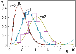
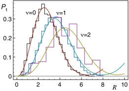
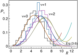
Figure 3: Integrated distribution $P_{1}(R)$ of the first eigenvalue for $\nu=0$, 1, 2 and $\mu a=0.1$ (left), $\mu a=0.3$ (middle), and $\mu a=1.0$ (right). The solid lines are the RMT results from Eq. (3), the the histograms are the lattice data of Ref. [9]. The bending-up of the RMT curves for large $R$ is an artifact of truncating the expansion (3). For $\mu a=1.0$ we also show the exact RMT results in the $\alpha\to\infty$ limit from Eq. (9).

The deviations of the theoretical curves from zero for large $R$ are an artifact of the truncation of the Fredholm determinant expansion. As $\mu$ (or $\alpha$) is increased, the convergence of the approximation becomes slower, i.e., more terms are needed.

For $\mu a=1.0$ we are almost in the radially symmetric regime. Thus we expect $P_{1}(R)$ computed approximately through Eq. (3) to be close to the exact result Eq. (9) in the $\alpha\to\infty$ limit. This expectation is confirmed in Fig. 3 (right).

5 Conclusions

In this work we have studied individual Dirac eigenvalue distributions in the $\epsilon$-regime of QCD at nonzero chemical potential. We provided a general framework for ordering complex eigenvalues. Our RMT computation for arbitrary $\alpha$ was based on the truncation of a Fredholm determinant expansion. In the $\alpha\to\infty$ limit, we were able to derive all IEDs analytically in closed form. These predictions were then tested against lattice data based on the generalization of the overlap Dirac operator to nonzero chemical potential, in the topological sectors $\nu=0$, 1, 2. We found excellent agreement between RMT and lattice results for several values of $\mu$ in the domain of the applicability of RMT. The descent of the IEDs represents a new, parameter-free test of RMT predictions. The much improved signal (resulting from the integration over the phase) allowed us, for the first time, to successfully test the RMT predictions in the topological sector $\nu=2$.