Alternating Heisenberg Spin-1/2 Chains in a Transverse Magnetic Field

Abstract

The ground state phase diagram of the alternating spin-1/2 chains with anisotropic ferromagnetic coupling under the influence of a symmetry breaking transverse magnetic field is studied. We have used the exact diagonalization technique. In the limit where the antiferromagnetic coupling is dominant, we have identified two Ising-type quantum phase transitions. We have calculated two critical fields $h_{c_{1}}$ and $h_{c_{2}}$, corresponding to the transition between different magnetic phases of the system. It is found that the intermediate state ($h_{c_{1}}<h<h_{c_{2}}$) is gapful, describing the stripe-antiferromagnetic phase.

1 Introduction

The effect induced by external magnetic fields in the low-dimensional magnets has attracted much interest recently from experimental and theoretical points of view. In particular, critical properties of the alternating spin-1/2 chains in a magnetic field have been a field of intense studies. This seems pertinent in the face of great progress made within the last years in fabrication of such AF-F compounds. Since, the AF-F chains have a gap in the spin excitation spectrum, they reveal extremely rich quantum behavior in the presence of the magnetic field.

A typical example of the ferromagnetic-dominant AF-F bond alternating chain is $\rm{(CH_{3})_{2}CHNH_{3}CuCl_{3}}$ (isopropylammonium coppertrichloride: $\rm{IPACuCl_{3}}$)[1, 2]. The energy gap in the absence of the external magnetic field is estimated from the susceptibility to be $17-18\rm{K}$[1]. This value is also confirmed by the analysis of the specific heat[2]. From the viewpoint of the crystal structure, the origin of the spin gap was expected to be the spin-1/ 2 AF-F alternating chain along the c-axis[1]. However, quite recently, it was suggested that this system should be characterized as a spin ladder along the a-axis with the strongly coupled ferromagnetic rungs, namely the antiferromagnetic chain with effective S = 1, and the excitation gap $\Delta$ was estimated as $13.6\rm{K}$ by means of the neutron inelastic scattering experiments.[3]

More recently, it was reported new inelastic neutron scattering results for $\rm{(CH_{3})_{2}NH_{2}CuCl_{3}}$ (Dimethylammonium copper II chloride, also known as: $\rm{DMACuCl_{3}}$ or MCCL). The linked-cluster calculations and the bulk measurements show that $\rm{DMACuCl_{3}}$ is a realization of the spin-1/2 alternating AF-F chain by nearly the same strength of the antiferromagnetic and ferromagnetic couplings.[4]

There are other examples for the AF-F alternating spin-1/2 chain compounds such as: $\rm{[Cu(TIM)]CuCl_{4}}$ (TIM=2,3,9,10-tetramethyl-1,3,8,10-tetraenecyclo-1,4,8,11-tetraazatetradecane) and $\rm{(4-BzpipdH)CuCl_{3}}$ (4-BzpipdH=4-benzylpiperidinium),[5, 6] and $CuNb_{2}O_{6}$[7].

Theoretically, the AF-F alternating chain is expected to have relation to the Haldane-gap systems[8], since they are regarded as the spin-1 antiferromagnetic chain in the large ferromagnetic coupling limit. The energy gap exist between the ground state and the first excited state. The spin correlation function of the ground state decays exponentially as well as the spin-1 AF chain. The ground state properties[9, 10, 11, 12, 13, 14, 15] and low-lying excitations[16] of this model were well investigated by numerical tools and variational schemes. In particular, the string order parameter originally defined for the spin-1 Heisenberg chains[17] was generalized to this system. The ground state has the long-range string order, which is characteristic of the Haldane-gap phase. Hida has shown that the Haldane phase of the AF-F alternating chain is stable against any strength of the randomness[18].

The ground state phase diagram of the AF-F alternating chain in a magnetic field is studied by the numerical diagonalization and the finite-size scaling based on the conformal field theory[12]. It is shown that the magnetic state is gapless and described by the Luttinger liquid phase. It is also found that the magnetic state is characterized by the algebraic decay of the spin correlation functions. Recently, Yamamoto et. al described the magnetic properties of the model in a magnetic field in terms of the spinless fermions and the spin waves[19]. They employed the Jordan-Wigner transformation and treated the fermionic Hamiltonian within the Hartree-Fock approximation. They have also implemented the modified spin wave theory to calculate the thermodynamic functions as the specific heat and the magnetic susceptibility.

The effect of an uniform transverse magnetic field on the ground state phase diagram of a spin-1/2 AF-F chain with anisotropic ferromagnetic coupling is much less studied. Partly, the reason is that AF-F alternating chains with anisotropic ferromagnetic coupling are not still fabricated. However, from the theoretical point of view these systems are extremely interesting, since they open a new wide polygon for the study of complicated quantum behavior, unexpected in the more conventional spin systems. The Hamiltonian of the model under consideration on a periodic chain of $N$ sites is given by

$$H = J_{AF}\sum_{j=1}^{N/2}[S_{2j-1}^{x}S_{2j}^{x}+S_{2j-1}^{y}S_{2j}^{y}+S_{2j-1}^{z}S_{2j}^{z}]$$ (1)

$$- J_{F}\sum_{j=1}^{N/2}[S_{2j}^{x}S_{2j+1}^{x}+S_{2j}^{y}S_{2j+1}^{y}+\Delta S_{2j}^{z}S_{2j+1}^{z}]$$

$$+ h\sum_{j=1}^{N}S_{j}^{x},$$

where $S_{j}^{x,y,z}$ are spin-1/2 operators on the $j$-th site. $J_{F}$ and $J_{AF}$ denote the ferromagnetic and antiferromagnetic couplings respectively. The limiting case of isotropic ferromagnetic coupling corresponds to $\Delta=1$ and $h$ is the transverse magnetic field. The model (1) in the case of $J_{F}=-J_{AF}$ and $\Delta=1$ corresponds to the isotropic Heisenberg chain in an external magnetic field. The ground state phase diagram of this model is known[20].

In this paper, we present our numerical results obtained in the low-energy states of the AF-F alternating spin-1/2 chain with anisotropic ferromagnetic coupling in a transverse magnetic field $h$. Assuming that the antiferromagnetic coupling is dominant, we study the effect of a uniform transverse magnetic field on the ground state phase diagram of the model. In particular, we apply the modified Lanczos method to diagonalize numerically finite chains. Using the exact diagonalization results, we calculate the spin gap, the magnetization, the string order parameter, and various spin-structure factors as a function of the uniform transverse magnetic field. Based on the exact diagonalization results we obtain the magnetic phase diagram of the model showing Haldane, stripe-antiferromagnetic and ferromagnetic phases. We denote by ”ferromagnetic phase” the phase with the magnetization parallel to the external field as only the nonvanishing order parameter. We show that the Haldane phase remains stable even in the presence of the uniform transverse field less than a critical field $h_{c_{1}}$.

The outline of the paper is as follows: In section II we discuss the model in the strong antiferromagnetic coupling limit and derive the effective spin chain Hamiltonian to outline the symmetry aspects of the problem. In section III we present results of the exact diagonalization calculations using the modified Lanczos method. Finally we conclude and summarize our results in section IV.

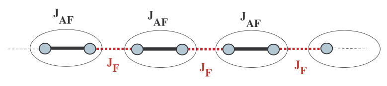
Figure 1: Sketch of the Spin-1/2 AF-F alternating Chain considered in this paper.

2 Large Antiferromagnetic Coupling Limit

In this section we will discuss the model (1) in the limiting case of the strong antiferromagnetic coupling $J_{AF}\gg J_{F}$. We will show that in this limit the model can be regarded as a fully anisotropic XYZ chain, which allows us to outline the symmetry aspects of the problem under consideration[21]. The schematic picture of the AF-F alternating chain is plotted in Fig. 1. At $J_{AF}\gg J_{F}$, the system behaves as the nearly independent block of pairs[22]. Indeed an individual block may be in a singlet ($|S>=1/\sqrt{2}[|\uparrow\downarrow>-|\downarrow\uparrow>]$) or a triplet state ($|T_{1}>=|\uparrow\uparrow>$, $|T_{0}>=1/\sqrt{2}[|\uparrow\downarrow>+|\downarrow\uparrow>]$, $|T_{-1}>=|\downarrow\downarrow>$) with the corresponding energies given by

$$E_{1,-1}=\left({J_{AF}\over 4}\ \mp h\right),\,\,E_{0}={J_{AF}\over 4},\,\,E_{s}=-{3J_{AF}\over 4}.$$

At $h\leq J_{AF}$, one component of the triplet becomes closer to the singlet ground state such that for a strong enough magnetic field we have a situation when the singlet and $S^{z}=1$ component of the triplet create a new effective spin $\tau=1/2$ system. One can easily project the original Hamiltonian (1) on the new singlet-triplet subspace

$$|\Downarrow\rangle\equiv|s\rangle=\frac{1}{\sqrt{2}}[|\uparrow\downarrow\rangle-|\downarrow\uparrow\rangle]\,,\qquad|\Uparrow\rangle\equiv|T_{1}\rangle=|\uparrow\uparrow\rangle\,.$$

When expressed in terms of the effective spin operators $\tau_{j}$ up to the accuracy of irrelevant constant, the original Hamiltonian (1) becomes the Hamiltonian of the spin-1/2 chain fully anisotropic XYZ chain in an effective magnetic field[22, 23]

$$H_{\emph{eff}} = \frac{J_{F}}{2}\sum_{j=1}^{N/2}[-\frac{1}{2}\tau^{z}_{j}\tau^{z}_{j+1}+\tau^{y}_{j}\tau^{y}_{j+1}+\Delta\tau^{x}_{j}\tau^{x}_{j+1}]$$ (2)

$$+ h^{eff}\sum_{j=1}^{N/2}\tau^{z}_{j}\,,$$

where $h^{eff}=h-J_{AF}+J_{F}/4$. Note that in deriving (2), we have used the rotation in the effective spin space which interchanges the $x$ and $z$ axes.

At $\Delta=1$, the effective problem reduces to the theory of the $XXZ$ chain with a fixed antiferromagneic anisotropy of $1/2$ in a magnetic field. The gapped phase at $h^{eff}<h^{eff}_{c_{1}}$ for the AF-F alternating chain corresponds to the negatively saturated magnetization phase for the effective spin chain, whereas the massless phase for the AF-F alternating chain corresponds to the finite magnetization phase of the effective spin-1/2 chain. The critical field $h^{eff}_{c_{2}}$ where the AF-F alternating chain is totally magnetized, corresponds to the fully magnetized phase of the effective spin-1/2 chain.

From the exact ground state phase diagram of the anisotropic $XXZ$ chain in a magnetic field [24], it is easy to check that $h^{eff}_{c_{1},c_{2}}=\mp J_{F}/4$. Therefore we can see that the isotropic AF-F alternating chain in a magnetic field shows a transition from the Haldane phase to the Luttinger-Liquid phase at $h_{c_{1}}=J_{AF}-J_{F}/2$ and a transition from the Luttinger-Liquid phase into the fully polarized phase at $h^{ext}_{c_{2}}=J_{AF}$.

Away from the isotropic point $\Delta=1$ the effective Hamiltonian (2) describes the fully anisotropic ferromagnetic XYZ chain in a magnetic field that is directed perpendicular to the easy axes. For the particular value of magnetic field $h^{eff}=0$, the effective XYZ chain is long range ordered in $"y"-$direction. This is corresponding to the original AF-F alternating chain being ordered in the direction perpendicular to the applied magnetic field with opposite staggered magnetization on the blocks. We have defined this new phase as a stripe-antiferromagnetic phase (Fig. 6). The stripe-antiferromagnetic phase extends over the whole region of the transverse magnetic field $h_{c_{1}}<h<h_{c_{2}}$. For other values of the $h^{eff}$ it is clear that the stripe-antiferromagnetic phase order will be replaced either by the Haldane phase ($h<h_{c_{1}}$ correspond to negative effective fields) or the phase with only one order parameter - magnetization along the applied field ($h>h_{c_{2}}$ correspond to positive effective fields).

Figure 2: Difference between the energy of the two lowest levels and the ground state energy as a function of the transverse magnetic field, $h$ for $J_{AF}=2J_{F}$ and $\Delta=0.5$ including different chain lengths $N=12,16,20$. The lowest three lines for $E_{1}-E_{0}$ are indistinguishable on this scale.

3 Numerical Results

In this section, for exploring the nature of the spectrum and the phase transition, we use the modified Lanczos method to diagonalize numerically finite chains ($N=12,16,20,24$). The energies of the few lowest eigenstates were obtained for the chains with periodic boundary conditions. To find the effect of a transverse magnetic field on the ground state phase diagram of the system, we start our consideration by the anisotropic case, $\Delta\neq 1$. First, we have computed the three lowest energy eigenvalues of $N=12,16,20$ chain with $J_{AF}=2J_{F}$ and different values of the anisotropy parameter $\Delta=0.25,0.5,0.75$. As an example, in Fig. 2 we have plotted results of this calculations for $\Delta=0.5$. It can be seen that the difference between the two lowest states, decreases by increasing the transverse magnetic field. These are independent of the chain length. Considering the limiting case of $J_{F}=0$ the system consists of the $N/2$ independent block of pairs. Indeed the energy of the ground state for the $N/2$ blocks is equal to $N/2\times E_{s}$, and in the presence of a magnetic field the first excited state has the energy equal to: $(N-1)/2\times E_{s}+E_{1}$. Thus the deference between two lowest energy of the system will be independent of the size of the system. However for the case of the $J_{AF}\gg J_{F}$ the other terms in the Hamiltonian behave as a small perturbation, which causes that the three lines for $E_{1}-E_{0}$ to be indistinguishable on this scale.

In the region of the magnetic fields $h_{c_{1}}<h<h_{c_{2}}$ the two lowest states form a twofold degenerate ground state in the thermodynamic limit. Thus, the excitation gap in the system is the difference between the second excited state and the ground state. In the case of the zero magnetic field ($h=0$) the spectrum of the model is gapped. The spectrum remains gapfull except at the two critical fields: $h_{c_{1}}=1.64\pm 0.01$ and $h_{c_{2}}=1.88\pm 0.01$. The spin gap, which appears at $h>h_{c_{1}}$, first increases vs external field, but then starts to decrease, and finally vanishes at $h_{c_{2}}$. At $h>h_{c_{2}}$ the gap opens again and, for a sufficiently large field becomes proportional to $h$. These results are in good agreement with the results obtained in the studies of the fully anisotropic antiferromagnetic $XYZ$ chain in a magnetic field [25].

On the other hand, we have also checked our numerical tools in the isotropic case, $\Delta=1$. In this case, we found that the gap decreases linearly and vanishes in the critical magnetic fields $h_{c_{1}}=1.57\pm 0.01$ and $h_{c_{2}}=2.0$, for the constant coupling $J_{AF}=2J_{F}$. Both values of the critical fields are obtained from studying of the finite chains are very close to the previous section results. Also, our numerical results showed that the spectrum remains gapless for $h_{c_{1}}<h<h_{c_{2}}$, in good agreement with numerical results reported by Sakai[12].

Figure 3: The transverse magnetization $M_{x}$ as a function of applied field $h$ for $N=20$ chain with $J_{AF}=2J_{F}$ and for different values of the anisotropy parameter $\Delta=0.25,0.50,0.75$.

To recognize the different phases induced by the transverse magnetic field in the ground state phase diagram, we have implemented the modified Lanczos algorithm of finite size chains $(N=12,16,20,24)$ to calculate the order parameters and the various spin correlation functions.

The first insight into the nature of the different phases can be obtained by studying the magnetization along the field axis

$$M^{x}=\frac{1}{N}\sum_{j}\left\langle S_{j}^{x}\right\rangle,$$ (3)

where the notation $\langle...\rangle$ represent the expectation value at the lowest energy state. In Fig. 3 we have plotted the magnetization along the applied transverse magnetic field, $M^{x}$, vs $h$ for the chain of length $N=20$. For arriving at this plot we considered $J_{AF}=2J_{F}$ for the different values of the anisotropy parameter $\Delta=0.25,0.5,0.75$. Due to the profound effect of the quantum fluctuations the transverse magnetization remains small but finite for $0<h<h_{c_{1}}$ and reaches zero at $h=0$. This is in agreement with the results of magnetization obtained in the case of fully anisotropic $XYZ$ chain [25]. Increasing the magnetic field, the magnetization increases for $h>h_{c_{1}}$ very fast. This behavior is in agreement with expectations, based on general statement that in the gapped phase, the magnetization along the applied field appears only at a finite critical value of the magnetic field equal to the spin gap. However, in finite systems we do not observe a sharp transition close to the saturation value, which happens at $h>h_{c_{2}}$. The values of the critical fields $h_{c_{1}}$ and $h_{c_{2}}$ depend on the anisotropy parameter $\Delta$. By increasing $\Delta$, the critical fields take larger values. Also, our numerical results show that the magnetization along the directions perpendicular to the applied field ($M^{y}$ and $M^{z}$) remains zero.

Figure 4: The string correlation function $O_{str}(l,N)$ for the $l=N/2$ as a function of the transverse magnetic field, $h$ for $J_{AF}=2J_{F}$ and $\Delta=0.5$ including different chain lengths $N=12,16,20,24$. The inset has shown the string order parameter, $O_{str}(N/2,N)$, as a function of the $1/N$ for a value of magnetic field $h=1.7>h_{c_{1}}$.

We employ the phenomenological renormalization group (PRG) method[26] to determine these critical fields ($h_{c_{1}}$, and $h_{c_{2}}$). In the disordered phase ($h_{c_{1}}>h$ or $h_{c_{2}}<h$), the gap ($E_{1}-E_{0}$) tend to a finite value so that $N(E_{1}-E_{0})$ increases with $N$. In the Ising phase $(E_{1}-E_{0})$ decreases exponentially with $N$ so that $N(E_{1}-E_{0})$ also decreases with $N$. The phenomenological renormalization group equation is:

Figure 5: Fixed points $h_{c_{1}}(N,N+4)$ and $h_{c_{2}}(N,N+4)$ of the phenomenological renormalization group equation for the energy gap, plotted versus $1/(N+2)$, for $J_{AF}=2J_{F}$ and $\Delta=0.5$ including different chain lengths $N=8,12,16,20,24$. The extrapolated values are: $h_{c_{1}}=1.64\pm 0.01$ and $h_{c_{2}}=1.88\pm 0.01$.

$$(N+4)g(N+4,h^{\prime})=Ng(N,h).$$ (4)

Where $g(N,h)=E_{1}(N,h)-E_{0}(N,h)$ is the gap value for chain length $N$ in the magnetic filed $h$. At the critical point, $N(E_{1}-E_{0})$ should be size independent for large enough systems in which the contribution from irrelevant operators is negligible. Due to this situation, we can accurately determine the critical points by the PRG method. We can define $h_{c}(N,N+4)$ as the $N$-dependent fixed point of Eq. 4 and it is extrapolated to the thermodynamic limit, in order to estimate $h_{c}$. At the critical point $h=h^{\prime}=h_{c}$, therefore the curves of $N(E_{1}-E_{0})$ vs. $h$ for sizes $N$ and $N+4$ cross at certain values $h_{c_{1}}(N,N+4)$ and $h_{c_{2}}(N,N+4)$ (’finite size critical points’). The thermodynamic critical points ($h_{c_{1}}$, and $h_{c_{2}}$) can be obtained by appropriately extrapolating $h_{c_{1}}(N,N+4)$ or $h_{c_{2}}(N,N+4)$ to $N\rightarrow\infty$. Figure (5) represents the extrapolation procedure of the transition points, for $J_{AF}=2J_{F}$ and $\Delta=0.5$ including different chain lengths $N=8,12,16,20,24$. The values of $h_{c_{1(2)}}(N,N+4)$ for four pairs of system sizes $(N,N+4)=(8,12),(12,16),(16,20)$, and $(20,24)$ are represented by square (circle) in this figure. The extrapolated values are: $h_{c_{1}}=1.64\pm 0.01$ and $h_{c_{2}}=1.88\pm 0.01$. The system size dependence of the critical points is almost negligible as shown in Fig. 5.

As we mentioned before, in the absence of the uniform transverse field, the spectrum is gapful. The ground state of the model is the Haldane phase with the long-range string order. Thus, the Haldane phase can be recognized from studying the string correlation function. The string correlation function in the chain of length $N$ defined only for odd $l$ as[18]

$$O_{str}(l,N)=-\left\langle exp\{i\pi\sum_{k=2j+1}^{2j+1+l}S^{z}_{k}\}\right\rangle.$$ (5)

In particular we have calculated the string correlation function $O_{str}(l,N)$ for the $l=N/2$. In Fig. 4 we have plotted $O_{str}(N/2,N)$ as a function of $h$ for the chain with $J_{AF}=2J_{F}$, $\Delta=0.5$ and for different values of the chain length $N=12,16,20,24$. As it can be seen from this figure, at $h<h_{c_{1}}$, $O_{str}(N/2,N)$ is close to its maximum value $1.0$, therefore the chain system is in the Haldane phase. The Haldane phase remains stable even in the presence of the transverse field less than $h_{c_{1}}$.

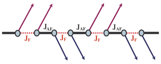
Figure 6: Classically, the long-range order canted in the direction of applied field $h$, which is expected in the ground state of the spin-1/2 AF-F alternating chain in a transverse field.

In the inset of the Fig. 4 we have also plotted the string order parameter, $O_{str}(N/2,N)$, as a function of the $1/N$ for a value of magnetic field $h=1.7>h_{c_{1}}$. It is clear that by increasing the size of the system, the $O_{str}(N/2,N)$, converges to the very small values close to zero. Which shows that there is not the string ordering at larger transverse magnetic fields $h>h_{c_{1}}$.

To get additional data about the character of the spin ordering in the intermediate gapped phase, we introduce a new order parameter. Classically, the effect of the transverse magnetic field $h$ is interesting. Energetically, the ground state of the system has a long-range order canted in the direction of the applied transverse magnetic field, as illustrated in Fig. 6. The ordering of this phase is a kind of the stripe-antiferromagnetic phase. Therefore the order parameter of the stripe-antiferromagnetic phase has been defined by

$$M_{st}^{y}=\frac{2}{N}\left\langle\sum_{j=1}^{N/2}(S_{2j-1}^{y}-S^{y}_{2j})(-1)^{j}\right\rangle.$$ (6)

For any value of the transverse field $h$ in the intermediate phase, the Lanczos results lead to $M_{st}^{y}=0$, since the ground state is two-fold degenerate and in a finite system no symmetry breaking happens . However the spin correlation function diverges in the ordered phase as $N\longrightarrow\infty$. We have computed the correlation function of the stripe-antiferromagnetic order parameter given by

$$\chi^{yy}=\left\langle\sum_{n=1}^{N/2}(S_{2j-1}^{y}-S^{y}_{2j})(S_{2j-1+2n}^{y}-S^{y}_{2j+2n})(-1)^{n}\right\rangle.$$ (7)

In Fig. 7 we have plotted $\chi^{yy}$ as a function of $h$ for the chain with $J_{AF}=2J_{F}$, $\Delta=0.5$ and for different values of the chain length $N=12,16,20,24$. As it is clearly seen from this figure, there is no long rang stripe-antiferromagnetic order along the $"y"$ direction at $h<h_{c_{1}}=1.65\pm 0.05$ and $h>h_{c_{2}}=1.90\pm 0.05$. However, in the intermediate region $h_{c_{1}}<h<h_{c_{2}}$, spins of each block show a profound antiferromagnetic order in the $"y"$ direction. Thus, between the critical fields $h_{c_{1}}$ and $h_{c_{2}}$, the ground state of the anisotropic case is Ising-type symmetry broken phase (stripe-antiferromagnetic phase) unlike the Luttinger liquid state for the isotropic case[12]. In the inset of Fig. 7 we have also shown the correlation function of the stripe-antiferromagnetic order $\chi^{yy}$ versus $N$ for a value of transverse field $h_{c_{1}}<h=1.8<h_{c_{2}}$. It can be seen that the function $\chi^{yy}$ shows the linear dependence on the chain length $N$, corresponding to the ordered stripe-antiferromagnetic phase in the intermediate region $h_{c_{1}}<h<h_{c_{2}}$.

Figure 7: The correlation function of the stripe-antiferromagnetic order parameter $\chi^{yy}$ as a function of the transverse magnetic field, $h$ for $J_{AF}=2J_{F}$ and $\Delta=0.5$ including different chain lengths $N=12,16,20,24$. In the inset the correlation function of the stripe-antiferromagnetic order $\chi^{yy}$ is plotted versus $N$ for a value of the transverse field $h_{c_{1}}<h=1.8<h_{c_{2}}$.

Thus, our numerical results show that the ground state phase diagram of the antiferromagnetic dominant spin-1/2 AF-F chain in a transverse field contains, besides the gapped Haldane and ferromagnetic phases, the stripe-antiferromagnetic phase. Each phase is characterized by its own type of long-range order: the ferromagnetic order along the transverse magnetic field axis in the ferromagnetic phase; the string order along the $"z"$ axis in the Haldane phase; and the stripe-antiferromagnetic order along the $"y"$ axis in the stripe-antiferromagnetic phase.

4 Conclusions

In this paper, we have investigated the ground state phase diagram of the antiferromagnetic dominant ($J_{AF}>J_{F}$) spin-1/2 AF-F chain with anisotropic ferromagnetic coupling in a transverse magnetic field $h$. We have implemented the modified Lanczos method to diagonalize numerically finite chains. Using the exact diagonalization results, we have calculated the various order parameters and the spin-structure factors as a function of the transverse magnetic field $h$. We have found that a gapped phase exists in the intermediate values of the transverse field ($h_{c_{1}}<h<h_{c_{2}}$). Then, we have identified its ordering as an interesting kind of the stripe-antiferromagnetic phase. Two quantum phase transitions in the ground state of the system with increasing transverse magnetic field have been identified. The first transition corresponds to the transition from the gapped Haldane phase to the gapped stripe-antiferromagnetic phase. The other one is the transition from the gapped stripe-antiferromagnetic phase into the fully polarized ferromagnetic phase.

On the other hand, in the limit that the antiferromagnetic coupling is dominant ($J_{AF}\gg J_{F}$) we have mapped the model (1), onto an effective XYZ Heisenberg chain in an external effective field ($h^{eff}$). This mapping allowed us to relate the critical fields $h_{c_{1}}$ and $h_{c_{2}}$ to the coupling constants in the isotropic case $\Delta=1$.

References

- [1] H. Manaka, I. Yamada, and K. Yamaguchi: J. Phys. Soc. Jpn. 66, (1997) 564.
- [2] H. Manaka, I. Yamada, Z. Honda, H. Aruga Katori, and K. Katsumata: J. Phys. Soc. Jpn. 67 (1998) 3913.
- [3] T. Masuda, A. Zheludev, H. Manaka, L. P. Regnault, J. H. Chung, and Y. Qiu: Phys. Rev. Lett. 96, (2006) 047210.
- [4] M. B. Stone, et. al: arXive:0705.0523v1 [cond-mat.str-el].
- [5] M. Hagiwara, Y. Narumi, K. Kindo, T. C. Kobayashi, H. Yamakage, K. Amaya, and G. Schumauch: J. Phys. Soc. Jpn. 66 (1997) 1792.
- [6] M. Takahashi, Y. Hosokoshi, H. Nakano, T. Goto, M. Takahashi, and M. Kinoshita: Mol. Cryst. Liq. Cryst. Sci. Technol., Sect. A 306 (1997) 111.
- [7] K. Kodama, H. Harashina, H. Sasaki, M. Kato, M. Sato, K. Kakurai, and M. Nishi: J. Phys. Soc. Jpn. 68 (1999) 237.
- [8] F. D. M. Haldane: Phys. Rev. Lett, 50 (1983) 1153.
- [9] S. Takada: J. Phys. Soc. Jpn. 61 (1992) 428.
- [10] K. Hida and S. Takada: J. Phys. Soc. Jpn. 61 (1992) 1879.
- [11] K. Hida: J. Phys. Soc. Jpn. 62 (1993) 439.
- [12] T. Sakai: J. Phys. Soc. Jpn. 64 (1995) 251.
- [13] K. Hida: Phys. Rev. B, 46 (1992) 8268.
- [14] M. Kohmoto and H. Tasaki: Phys. Rev. B, 46 (1992) 3486.
- [15] M. Yamanaka, Y. Hatsugai, and M. Kohmoto: Phys. Rev. B, 48 (1993) 9555.
- [16] K. Hida: J. Phys. Soc. Jpn. 63 (1994) 2514.
- [17] M. den Nijs and K. Rommelse: Phys. Rev. B, 40 (1989) 4709.
- [18] K. Hida: Phys. Rev. Lett, 83 (1999) 3297.
- [19] S. Yamamoto et. al,: Fiz. Nizk. Temp. 31 (2005) 974.
- [20] D. V. Dmitriev, V. Ya. Krivnov, and A. A. Ovchinnikov: Phys. Rev. B, 65 (2002) 172409.
- [21] G. I. Japaridze, A. Langari, S. Mahdavifar: J. Phys.: Condens. Matter, 19 (2007) 076201.
- [22] F. Mila: Eur. Phys. J. B, 6 (1998) 201.
- [23] K. Totsuka: Phys. Rev. B 57, (1998) 3454.
- [24] Takahashi M: Thermodynamics of one-dimensional solvable models, (Cambridge: Cambridge University Press) Chapter IV (1999).
- [25] Hogemans R, Caux J-S, and Löw U: Phys. Rev. B, 71 (2005) 014437.
- [26] M. N. Barber: Phase Transitions and Critical Phenomena 8, edited by C. Domb and J. L. Lebowitz (Academic Press, London, New York, 1983), 146.