Formulating Light Cone QCD on the Lattice

Abstract

We present the near light cone Hamiltonian $H$ in lattice QCD depending on the parameter $\eta$, which gives the distance to the light cone. Since the vacuum has zero momentum we can derive an effective Hamiltonian $H_{eff}$ from $H$ which is only quadratic in the momenta and therefore solvable by standard methods. An approximate ground state wave functional is determined variationally in the limit $\eta\rightarrow 0$.

I Introduction

The lattice approach to QCD pioneered by Wilson wilson and first realized numerically by Creutz creutz is based on the QCD action. Moreover, it has been mainly developed in an Euclidean path integral formulation. In contrast to that, Hamiltonian techniques have remained less studied. With the Hamiltonian, one can project out the correct ground state by evolving an initial wave functional in imaginary time. In continuum theory, some progress has been made recently in the non-perturbative regime Feuchter:2004mk ; Leigh:2005dg ; Greensite:2007ij . Accoring to these circumstances there have been only few contacts between lattice QCD and light cone field theory (LCFT).

There is no doubt that LCFT is an important tool for the description of high energy interactions. The knowledge of wave functionals in the gauge field configuration space may help to calculate light cone wave functions of hadrons. In the following paper we attempt to take advantage of lattice methods in LCFT (for previous work, see Mustaki:1988gi ; Bardeen:1979xx ; Burkardt:2001jg ; Dalley:2003aj ). Although the Hamiltonian is not Lorentz invariant, the light cone Hamiltonian Burkardt:2001jg ; pauli offers the advantage of being boost invariant and has – naively interpreted – a trivial vacuum. On the other hand, one would be surprised if QCD looses its non-perturbative vacuum structure in the light cone limit. In our opinion much of the complicated vacuum structure of QCD is hidden in the constraint equations appearing in light cone QCD. The constraint equations contain zero mode solutions which are difficult to solve. These quantum constraint equations have been attacked in lower dimensions for scalar theories, but gauge theories still escape a solution in higher dimensions. In Nambu Jona Lasinio models Lenz:2004tw one has been able to solve these zero mode equations in the large $N_{c}$ approximation.

A quantization of scalar light cone field theory on the lattice has been first analysed in ref. Mustaki:1988gi where also the time coordinate has been discretized. In this reference, special care has been devoted to the constraints which arise on the light cone. This approach has not found applications. In particular, it is not easily extendable to gauge theories.

Remarkable progress has been made in light cone QCD with a color dielectric lattice theory as a starting point Bardeen:1979xx ; Dalley:2003aj ; Dalley:2003uj . This approach is based on “fat” links which arise from averaging gluon configurations by a block spinning procedure Mack:1983yi ; Pirner:1991im . With this method the spectrum of glue balls and the pion light cone wave function have been calculated Dalley:2002nj . In a Lagrangian framework the connection to the original QCD Lagrangian can be easily made, although the numerical accuracy is limited. On the light cone, however, one is prevented from approaching the continuum limit, since an effective potential for the link matrices $M\in GL(N)$ with a non vanishing vacuum expectation value is not allowed. The norm of the link matrices $M\in GL(N)$, however, should approach unity in the continuum limit.

This is the reason why we propose to formulate QCD near the light cone. We have already analyzed scalar theories Prokhvatilov:1994dm and QCD Naus:1997zg ; Ilgenfritz:2000bj approaching the light cone in a tilted near light cone reference system containing a parameter $\eta\neq 0$ parameterizing the distance to the light cone. Our work in this paper will follow this idea deriving a lattice Hamiltonian which describes the pure gauge sector of QCD and which is suitable for a numerical treatment. For QCD, we have already followed the path of maximal gauge fixing Naus:1997zg ; Ilgenfritz:2000bj outlined by the Erlangen group lenz in previous works. This way to eliminate all gauge degrees of freedom looks very attractive analytically, but numerically it is not advantageous. It includes solutions of constraint equations which complicate the form of the Hamiltonian. Hence we do not fix the gauge in the following work and try to establish a form of the Hamiltonian describing the near light cone dynamics similar to the QCD Hamiltonian in an equal time approach, i.e. in terms of unitary matrices describing the gauge degrees of freedom and their canonically conjugate momenta. In our lattice prescription, we leave near light cone time continuous. It plays a similar role as ordinary Minkowski time, therefore, we can follow the conventional method of the transfer matrix in order to derive the lattice Hamiltonian from the lattice action. The transversal field strengths are increased in magnitude due to the boost into the vicinity of the light cone whereas the longitudinal fields remain unchanged. Constraint equations arise in the light cone Hamiltonian framework, since the Lagrangian contains the velocities in linear form. The momenta related to these velocities obey constraint equations. The constraint equations appear in the near light cone Hamiltonian as terms proportional to $1/\eta^{2}$. These terms enforce the “equality” of the transverse chromo electric and chromo magnetic fields $E_{k}^{a}=F_{-k}^{a}$. While the longitudinal chromo electric field and the longitudinal chromo magnetic field appear in their usual form in the light cone Hamiltonian, the Hamiltonian contains the transverse chromo magnetic field squared in an unusual quadratic $Z(2)$ invariant form. The $Z(2)$ invariance, however, is broken because the chromo magnetic fields also appear linearly together with the transverse chromo electric field.

The lattice Hamiltonian density depends on an effective constant which represents the product of the anisotropy parameter $\xi=a_{-}/a_{\bot}$ and the near light cone parameter $\eta$. If one chooses $\eta=1$ and lets $\xi\rightarrow 0$ one obtains a deformed system which is squeezed in the spatial ($-$)-direction, if one uses $\xi=1$ and lets $\eta\rightarrow 0$ one obtains the light cone limit. This equivalence has been advocated before by Verlinde and Verlinde Verlinde:1993te and Arefeva Arefeva:1993hi . These authors have proposed to implement the strong interaction with such asymmetric lattices in order to study high energy scattering, motivating us to proceed in this way. As it stands, the (anisotropic) lattice Hamiltonian itself is not usable for Monte Carlo methods evolving an arbitrary initial state in imaginary time to the ground state, since the chromo electric field strengths i.e. the momenta canonically conjugate to the links appear linearly. Therefore we propose to use the translational invariance of the vacuum to add a term $1/\eta^{2}P_{-}$ in order to cancel the unwanted terms. Naively this amounts to returning to an effective lattice Hamiltonian which is proportional to the energy in ordinary Minkowski coordinates. For the ground state of the vacuum this seems a reasonable procedure. Applications of the light cone coordinates in finite temperature field theory have followed the same route Raufeisen:2004dg . The new effective Hamiltonian contains two parts: The first describing the dynamics of the longitudinal chromo electric and chromo magnetic fields is not influenced by the smallness of the near light cone parameter $\eta$. The second part containing the transverse chromo electric and chromo magnetic terms is enhanced with $\eta$ in the light cone limit.

We analytically investigate this effective Hamiltonian in the strong and weak coupling limit. Such a procedure can direct the search for an appropriate (approximate) guidance wave functional needed to improve the convergence of the Hamiltonian Monte Carlo method. The strong coupling limit suggests a simple sum of plaquette terms with different weights in the purely transverse and ($-$)-transverse planes. The magnitude of the couplings follows the asymmetries existing in the Hamiltonian. In the limit $\eta\rightarrow 0$ the plaquette terms in the purely transverse planes are weighted very weakly, i.e. the longitudinal magnetic fields can vary freely. The weak coupling approximation identifies the “abelian” fluctuations with their modified dispersion relations following the built in anisotropy. It is particularly interesting that the light cone limit $\eta\rightarrow 0$ produces long-range correlations in the minus direction, which deviate from the local strong coupling ansatz. In fact this anisotropy may help to make an ansatz for the ground state wave functional which is especially appropriate in the light cone limit. It correlates fluctuations of the longitudinal chromo magnetic fields with long strings along the ($-$)-direction. This ansatz may also point the way to find a solution of the quantum constraint of the initial Hamiltonian.

The outline of the paper is as follows: In Sec. II we introduce near light cone coordinates. For the sake of clarity, we first establish the methodology in the continuum formulation. We derive the continuum Hamiltonian and momentum operator. Furthermore, we motivate an effective Hamiltonian making an ordinary Quantum Diffusion Monte Carlo algorithm possible. In Sec. III we switch to the lattice formulation and derive the near light cone Hamiltonian from the latticized action with the transfer matrix method. In Sec. IV we set up the effective Hamiltonian. The time independent Schrödinger equation for the effective Hamiltonian is analytically solved for the ground state in the strong and weak coupling limit in Sec. V. In Sec. VI we variationally optimize an ansatz for the ground state wave functional motivated by the strong and weak coupling analysis. It allows to interpolate between these two extreme limits and to investigate the $\eta$ behavior in the whole coupling range. Finally, in Sec. VII, we present our conclusions and an outlook to future work.

II The continuum QCD Hamiltonian and momentum near the light cone

Before we start with the actual derivation of the QCD Hamiltonian and momentum near the light cone, we would like to introduce near light cone coordinates similar to the coordinates first proposed by Prokhvatilov:1989eq ; Lenz:1991sa . The transition to near light cone (nlc) coordinates might be considered as a two-step process. In the first step, one starts in ordinary Minkowski space in the laboratory frame with unprimed coordinates $x^{\mu}$ and transforms into a reference frame described by primed coordinates $x^{\prime\mu}$ which moves with relative velocity $\beta$ along the longitudinal direction relative to the laboratory frame. The relative velocity $\beta$ is chosen to be given by

$$\beta = \frac{1-\eta^{2}}{1+\eta^{2}}\;,\;\eta~{}\in~{}\left[0,1\right].$$ (1)

The associated Lorentz transformation expressing the primed coordinates in terms of laboratory frame coordinates reads

$$x^{\prime 0} = \gamma\left(x^{0}-\beta\,x^{3}\right)$$

$$x^{\prime 3} = \gamma\left(x^{3}-\beta\,x^{0}\right)\;,\;\gamma=\left(1-\beta^{2}\right)^{-1/2}\;.$$ (2)

Here $x^{0}$ and $x^{3}$ denote the temporal coordinate and the longitudinal spatial coordinate respectively in usual Minkowski coordinates. From the boosted frame, one performs an additional linear transformation not included in the Lorentz group which rotates the temporal and longitudinal coordinates. It is given by

$$x^{+} = \frac{1}{2}\Bigl{[}\left(1+\eta^{2}\right)x^{\prime 0}+\left(1-\eta^{2}\right)x^{\prime 3}\Bigr{]}$$

$$x^{-} = \phantom{\frac{1}{2}}\Bigl{[}x^{\prime 0}-x^{\prime 3}\Bigr{]}\;.$$ (3)

Here, $x^{+}$ is defined to be the new time coordinate along which the system evolves and $x^{-}$ is defined to be the new spatial longitudinal coordinate. The transversal coordinates $x^{1}$ and $x^{2}$ remain unchanged. By quantizing a theory on a hypersurface of constant $x^{+}$, one can smoothly interpolate between an equal time quantization and light cone quantization by varying the external near light cone parameter $\eta$ from $1$ to $0$. In the equal time limit $\eta=1$, the temporal coordinate $x^{+}$ is given by the ordinary Minkowski time coordinate $x^{+}=x^{0\prime}$ and $\beta=0$, i.e. the new reference frame is not moving relative to the laboratory frame. In the light cone limit $\eta\rightarrow 0$, $x^{+}$ is proportional to the usual temporal light cone coordinate and $\beta$ approaches $\beta=1$. The nlc energy $p_{+}$ and longitudinal momentum $p_{-}$ expressed in terms of the laboratory energy $E$ and longitudinal momentum $p^{3}$ are given by

$$p_{+} = \frac{1}{\eta}\left(E-p^{3}\right)$$

$$p_{-} = \eta\,p^{3}\;.$$ (4)

The second relation in Eq. (4) shows that the magnitude of longitudinal momenta is reduced by transforming to nlc coordinates. In other words, large longitudinal momenta in the lab frame $p^{3}\propto 1/(a_{-}\eta)$ become accessible by a nlc lattice with longitudinal lattice spacing $a_{-}$ for $\eta\rightarrow 0$. This makes nlc coordinates physically very attractive.

The definition of nlc coordinates Eq. (3) induces the following metric:

$$\begin{array}[]{cc}g_{\mu\nu}=\left(\begin{array}[]{cccc}0&0&0&1\\ 0&-1&0&0\\ 0&0&-1&0\\ 1&0&0&-\eta^{2}\end{array}\right)&g^{\mu\nu}=\left(\begin{array}[]{cccc}\eta^{2}&0&0&1\\ 0&-1&0&0\\ 0&0&-1&0\\ 1&0&0&0\end{array}\right)\end{array}$$ (5)

with $\mu,\nu=+,1,2,-,\det g=1$. This defines the scalar product

$$x_{\mu}y^{\mu} = x^{-}y^{+}+x^{+}y^{-}-\eta^{2}x^{-}y^{-}-\vec{x}_{\perp}\vec{y}_{\perp}$$ (6)

$$= x_{-}y_{+}+x_{+}y_{-}+\eta^{2}x_{+}y_{+}-\vec{x}_{\perp}\vec{y}_{\perp}\;.$$

Note, that the metric has off-diagonal terms which implies that there are terms mixing temporal and longitudinal spatial coordinates in the scalar product. This has severe consequences for a standard Euclidean lattice approach.

If we put a pair of color charges propagating along the longitudinal coordinate $x^{-}$ described by a longitudinally extended Wegner-Wilson loop and a stationary target modeled by a transversal plaquette at fixed $x^{-}$ in this reference frame, we can simulate color dipoles colliding with a hadron Iancu:2002xk in the light cone limit. In the described way one might be able to calculate cross sections between hadrons. For $\eta\rightarrow 0$, we approach the light cone from space like distances which is different from the approach of Balitsky Babansky:2002my who approaches the light cone from time like distances closer to scattering experiments.

For QCD, the pure gluonic part of the Lagrange density in manifestly covariant notation is given by

$$\mathcal{L} = -\frac{1}{4}F_{\mu\nu}^{a}g^{\mu\kappa}g^{\nu\rho}F_{\kappa\rho}^{a}\;,$$ (7)

with the non-abelian field strength tensor

$$F_{\mu\nu}^{a} \equiv \partial_{\mu}A_{\nu}^{a}-\partial_{\nu}A_{\mu}^{a}+gf^{abc}A_{\mu}^{b}A_{\nu}^{c}\;.$$ (8)

In the following, we restrict ourselves to the color gauge group $SU(2)$ for which the structure constants $f^{abc}$ are given by the three-dimensional totally antisymmetric Levi-Cevita symbol $\epsilon^{abc}$. By using the nlc metric Eq. (5) we obtain for the Lagrange density Eq. (7)

$$\mathcal{L} = \sum\limits_{a}\left[\frac{1}{2}F_{+-}^{a}F_{+-}^{a}+\sum\limits_{k=1}^{2}\left(F_{+k}^{a}F_{-k}^{a}+\frac{\eta^{2}}{2}F_{+k}^{a}F_{+k}^{a}\right)-\frac{1}{2}F_{12}^{a}F_{12}^{a}\right]\;.$$ (9)

Note, that there is a term in the Lagrange density which is only linear in one of the temporal field strengths, namely $F_{+k}^{a}F_{-k}^{a}$. Therefore, the numerical standard approach for lattice gauge theory, the Monte Carlo sampling of the Euclidean path integral does not apply for nlc coordinates. The reasoning is as follows. If one performs in analogy to equal time theories an analytical continuation to imaginary nlc time $x^{+}\rightarrow-\mathrm{i}x^{+}_{E}$, each temporal field strength is replaced by its Euclidean counterpart times an additional factor $\mathrm{i}$. Therefore, the linear term yields a complex valued Euclidean action and the integrand of the Euclidean path integral is no longer interpretable as a probability density. A similar problem arises for lattice gauge theory at finite baryonic densities which is usually referred to as the sign problem. So far, no convenient solution has been found. In order to avoid these problems, we stay in Minkowski time for the rest of the paper and we switch to a Hamiltonian formulation. We perform a Legendre transformation to switch to a Hamiltonian formulation , i.e. we have to express the temporal derivatives of the fields by their canonical conjugate momenta in particular which are given by the functional derivatives of the Lagrange density with respect to the temporal derivative of the correspondent fields:

$$\Pi_{\mu}^{a} \equiv \frac{\delta\mathcal{L}}{\delta\left(\partial_{+}A_{\mu}^{a}\right)}\;.$$ (10)

Therefore, the canonical momenta conjugate to the gauge fields are given by

$$\Pi_{k}^{a} = \frac{\delta\mathcal{L}}{\delta\partial_{+}A_{k}^{a}}=\frac{\delta\mathcal{L}}{\delta F_{+k}^{a}}=F_{-k}^{a}+\eta^{2}F_{+k}^{a}\;,$$

$$\Pi_{-}^{a} = \frac{\delta\mathcal{L}}{\delta\partial_{+}A_{-}^{a}}=\frac{\delta\mathcal{L}}{\delta F_{+-}^{a}}=F_{+-}^{a}\;.$$ (11)

Here, we have chosen the axial gauge $A_{+}^{a}=0$ which is quite natural because the temporal gauge field $A_{+}^{a}$ is not dynamical, i.e. there is no temporal derivative appearing in the Lagrange function. It acts like a Lagrange multiplier which multiplies the Gauss law $G=0$ with $G$ given by:

$$G = D_{-}^{ac}\;\Pi_{-}^{c}+D_{k}^{ac}\;\Pi_{k}^{c}\;.$$ (12)

Here $D_{\mu}^{ac}$ denotes the ordinary covariant derivative - in the adjoint representation - in spatial direction $\mu$

$$D_{\mu}^{ac} = \partial_{\mu}\delta^{ac}+gf^{abc}A_{\mu}^{b}\;.$$ (13)

In order to recover the full Lagrangian dynamics, we have to supplement the equations of motion by Gauss’ law. Hence, the Gauss law has to be imposed as a constraint equation on physical states. We express the temporal derivatives of the gauge fields in terms of the canonical conjugate momenta by using Eq. (11), which yields

$$\partial_{+}A_{k}^{a} = F_{+k}^{a}=\frac{1}{\eta^{2}}\left(\Pi_{k}^{a}-F_{-k}^{a}\right)\;,$$

$$\partial_{+}A_{-}^{a} = F_{+-}^{a}=\Pi_{-}^{a}\;.$$ (14)

We may obtain the QCD Hamiltonian and the momentum operator via the energy momentum tensor, where we have to substitute the temporal derivatives of the gauge fields by the corresponding expressions involving the canonical conjugate momenta Eq. (14). If the Lagrange density for an arbitrary field theory with fields $\Phi_{r}$ defined by the Lagrangian density $\mathcal{L}$ is a function of the fields itself and derivatives of the fields only, namely $\mathcal{L}=\mathcal{L}(\Phi_{r},\partial_{\mu}\Phi_{r})$, the energy momentum tensor in its most general form is given by

$$T^{\mu\nu} = \sum\limits_{r}\frac{\delta\mathcal{L}}{\delta\left(\partial_{\mu}\Phi_{r}\right)}\partial^{\nu}\Phi_{r}-g^{\mu\nu}\mathcal{L}\;,$$ (15)

It defines the Hamiltonian density $\mathcal{H}$ and the longitudinal momentum density $\mathcal{P}_{-}$ by

$$\mathcal{H} = T_{\;\;\;+}^{+}\;,$$

$$\mathcal{P}_{-} = T_{\;\;\;-}^{+}\;.$$ (16)

Therefore, for the nlc QCD Lagrangian Eq. (9) we find the Hamiltonian density

$$\mathcal{H} = \frac{1}{2}\sum\limits_{a}\left[\Pi_{-}^{a}\Pi_{-}^{a}+F_{12}^{a}F_{12}^{a}+\sum\limits_{k=1}^{2}\frac{1}{\eta^{2}}\left(\Pi_{k}^{a}-F_{-k}^{a}\right)^{2}\right]$$ (17)

and the longitudinal momentum density

$$\mathcal{P}_{-} = \Pi_{-}^{a}\partial_{-}A_{-}^{a}+\sum\limits_{k=1}^{2}\Pi_{k}^{a}\partial_{-}A_{k}^{a}\;.$$ (18)

This form of the local integrand for the generator $\mathcal{P}_{-}$ of longitudinal translations is not manifestly gauge invariant. However, if one uses Gauss’ law and the definition of the field strength tensor one can rewrite $\mathcal{P}_{-}$ as

$$\mathcal{P}_{-} = \Pi_{k}^{a}F_{-k}^{a}+\partial_{k}\left(\Pi_{k}^{a}A_{-}^{a}\right)+\partial_{-}\left(\Pi_{-}^{a}A_{-}^{a}\right)\;.$$ (19)

So, the longitudinal momentum density $\mathcal{P}_{-}$ may be expressed as a manifestly gauge invariant object plus some total derivatives along the spatial directions which disappear after integration with periodic boundary conditions. We use the symmetrized form

$$\mathcal{P}_{-} = \frac{1}{2}\left(\Pi_{k}^{a}F_{-k}^{a}+F_{-k}^{a}\Pi_{k}^{a}\right)\;.$$ (20)

The integrated Hamiltonian density ${H}$ is the generator of nlc “time” translations and the integrated longitudinal momentum operator ${P}_{-}$ is the generator of spatial translations in longitudinal direction:

$${H} = \int d^{2}x_{\bot}dx^{-}{\mathcal{H}}\;,$$

$${P}_{-} = \int d^{2}x_{\bot}dx^{-}{\mathcal{P}}_{-}\;.$$ (21)

We quantize the theory by choosing the following commutation relations at equal light cone time $x^{+}$ :

$$\left[{\Pi}_{m}^{a}(\vec{x}),{A}_{n}^{b}(\vec{y})\right] = -\mathrm{i}\delta^{ab}\delta_{mn}\delta^{(3)}(\vec{x}-\vec{y})\;,$$

$$\left[{\Pi}_{m}^{a}(\vec{x}),{\Pi}_{n}^{b}(\vec{y})\right] = 0\;,$$

$$\left[{A}_{m}^{a}(\vec{x}),{A}_{n}^{b}(\vec{y})\right] = 0\;.$$ (22)

These commutator relations respect the Heisenberg equations of motion. Note, analogously for Quantum Mechanics, one has to supplement the Heisenberg equations of motion by the Gauss law constraint. In quantum mechanics, the Gauss law constraint translates into a restriction of the Hilbert space to the subspace of physical states i.e. states $\Psi$ satisfying the Gauss law

$$\left({D}_{-}^{ab}{\Pi}_{-}^{b}(\vec{x})+\sum\limits_{k=1}^{2}{D}_{k}^{ab}{\Pi}_{k}^{b}(\vec{x})\right)\left|\Psi\right\rangle = 0\;\;\;\;\forall\;\vec{x},a\;.$$ (23)

Since the Gauss law operator is the generator of gauge transformations the physical subspace is given by that part of the entire Hilbert space which is spanned by gauge invariant states.
The $1/\eta^{2}$-term in the Hamiltonian Eq. (17) favors expectation values of transverse chromo electric fields $\Pi_{k}^{a}$ and transverse chromo magnetic fields $F_{-k}^{a}$ to be equal in order to have a minimal energy. On the other hand, this term introduces terms linear in momentum which are difficult to handle, for example with a numerical Quantum Diffusion Monte Carlo algorithm Chin:1983pc ; Chin:1985ua ; Heys:1984kg which exploits the fact that the time evolution operator is a projector onto the ground state when analytically continued to imaginary times. The terms linear in the momentum enforce the wave functional to be complex valued in general which spoils the whole procedure. These are exactly the same terms which make the nlc action complex valued after the Wick rotation in the action based formulation. Hence, the problem reappears in the Hamiltonian formulation. However, for Hamiltonian nlc QCD it is possible to define an effective Hamiltonian converging to the exact ground state which avoids the problematic terms.
Obviously, the Hamilton operator ${H}$ in Eq. (21) is translation invariant and gauge invariant. Hence, it commutes with the longitudinal momentum operator ${P_{-}}$ and with the Gauss operator $G$:

$$\left[{H},{P}_{-}\right] = 0\;,$$

$$\left[{H},G\right] = 0\;.$$ (24)

Therefore, common eigenstates exist which diagonalize the Hamiltonian and the longitudinal momentum operator simultaneously and in addition fulfill the Gauss law. In particular, momentum is a good quantum number which is left invariant by time evolution. In order to solve the Hamiltonian we are interested in translation-invariant states which are eigenstates of the longitudinal momentum operator, i.e. with eigenvalue equal zero. In vacuum, with light cone momentum $P_{-}=0$, we can add $(1/\eta^{2})~{}P_{-}$ to define an effective Hamiltonian density $\mathcal{H}_{eff}$ which is only quadratic in momenta:

$$\mathcal{H}_{eff} = \mathcal{H}+\frac{1}{\eta^{2}}\mathcal{P}_{-}$$ (25)

$$= \frac{1}{2}\sum\limits_{a}\left[\Pi_{-}^{a}\Pi_{-}^{a}+F_{12}^{a}F_{12}^{a}+\sum\limits_{k=1}^{2}\frac{1}{\eta^{2}}\left(\Pi_{k}^{a}\Pi_{k}^{a}+F_{-k}^{a}F_{-k}^{a}\right)\right]\;.$$

This effective Hamiltonian density is still symmetric under the exchange

$$\Pi_{k}^{a}\longleftrightarrow F_{-k}^{a}\;,$$ (26)

but it does not enforce the equality between transverse chromo electric and transverse chromo magnetic fields commonly used in the light cone limit also for the quantum field theoretic system.
One finds the ground state $\left|\Psi_{0}\right\rangle$ of ${H}$ by evolving a translation invariant trial state $\left|\Phi\right\rangle$ not orthogonal to $\left|\Psi_{0}\right\rangle$ with the effective time evolution operator

$$\left|\Psi_{0}\right\rangle = \lim_{\tau\rightarrow\infty}\exp\left[-\left({H}_{eff}-E_{eff}\right)\tau\right]\left|\Phi\right\rangle$$ (27)

related to the effective Hamiltonian. For the details of an explicit implementation of the ground state projection operator with a guided Quantum Diffusion Monte Carlo algorithm, we refer the reader to Chin:1983pc ; Chin:1985ua ; Heys:1984kg . In order to direct the Monte Carlo into regions of the configuration space which have large acceptance rates, i.e. which have a large exact ground state probability density for the given configuration, one introduces a guidance wave functional which is an approximation of the exact ground state. Instead of evolving the trial state itself, one evolves a probability density in imaginary time which converges to the product of the exact ground state wave functional and the guidance wave functional for asymptotic times. Obviously, the application of a guidance wave functional introduces some bias in the computation of expectation values. However, in principle one can get rid of this bias by applying forward walking techniques Ceperley:1979 ; Hamer:2000em .
The algorithm preserves Gauss’ law as long as the guidance/trial wave functional is a functional of closed loops only. In principle, there are also multiple connected loops possible, but then the chromo electric flux must be conserved at each site. In this paper our primary objective is to translate the discussed methodology onto the lattice and to determine variationally a good starting and guidance wave functional $\left|\Phi\right\rangle$ for the Quantum Diffusion Monte Carlo evolution based on Eq. (27) which is motivated by analytical computations in the strong and weak coupling limit.

III Near light cone Hamiltonian ${H}$ on the lattice

In order to regularize the continuum formulation we go over to the lattice formulation. In a previous paper Ilgenfritz:2006ir we have started deriving the Hamiltonian for gauge theories on the lattice from the path integral via the transition $a_{+}\rightarrow 0$. Here, we go through the procedure in detail. We introduce in four-dimensional space $SU(N)$ link variables $U_{i}(x)$ connecting the site $x$ with the 4D site $x+\widehat{e}_{i}$ ($\widehat{e}_{i}$, $i=+,-,1,2$, is a unit vector in 4D space-time) in the following way:

$$U_{i}(x) \equiv \mathcal{P}\exp\left(\mathrm{i}~{}g\int\limits_{x}^{x+\widehat{e}_{i}}dy^{\mu}~{}A_{\mu}^{a}(y)~{}\frac{\sigma_{a}}{2}\right)\;,$$ (28)

where $\mathcal{P}$ is implementing path ordering from left to right with increasing $y^{\mu}$ and $\sigma_{a}$ are hermitian color generators. In the following, we restrict to $SU(2)$ where the $\sigma_{a}$ are given by the Pauli matrices. The hermitian conjugate of the link variables, $U_{i}^{\dagger}(x)$, connect the site $x+\widehat{e}_{i}$ with the site $x$ in reverse order. Plaquettes $U_{ij}(x)$ are related to the field strengths $F_{ij}(x)$ and have the usual form

$$U_{ij}(x)=U_{i}(x)U_{j}(x+\widehat{e}_{i})U_{i}^{\dagger}(x+\widehat{e}_{j})U_{j}^{\dagger}(x)~{}.$$ (29)

Expanding a plaquette around its center $x+\frac{\widehat{e}_{i}}{2}+\frac{\widehat{e}_{j}}{2}$ in orders of the lattice spacing one obtains

$$U_{ij}(x)=\mathds{1}+\mathrm{i}ga_{i}a_{j}F_{ij}^{a}\frac{\sigma_{a}}{2}-\frac{1}{2}g^{2}a_{i}^{2}a_{j}^{2}F_{ij}^{a}F_{ij}^{b}\frac{\sigma_{a}}{2}\frac{\sigma_{b}}{2}+\ldots~{}.$$ (30)

Here $a_{i}$ denotes the lattice spacing for direction $i$, i.e. we allow in general for different lattice spacings in the temporal, longitudinal and transversal directions. A correspondent expansion is obtained for $U_{ij}^{\dagger}(x)$. Therefore, the sum over color indices $a=b$ of a product of field strengths is given in the limit $a_{i}\rightarrow 0$ as follows

$$F_{ij}^{a}F_{ij}^{a}(x)=\frac{4}{g^{2}a_{i}^{2}a_{j}^{2}}~{}\mathrm{Tr}\left[\,\mathds{1}-\mathrm{Re}\Big{(}\,U_{ij}(x)\,\Big{)}\,\right]\;.$$ (31)

Or more general

$$F_{ij}^{a}F_{kl}^{a}(x)=\frac{2}{g^{2}a_{i}a_{j}a_{k}a_{l}}\mathrm{Tr}\left[\,\mathrm{Im}\Big{(}\,U_{ij}(x)\,\Big{)}~{}\mathrm{Im}\Big{(}\,U_{kl}(x)\,\Big{)}\,\right]\;.$$ (32)

Here, $\mathrm{Re}\left(U\right)$ and $\mathrm{Im}\left(U\right)$ are defined as

$$\centering\mathrm{Re}\left(U\right)\equiv\frac{U+U^{\dagger}}{2}\@add@centering \mathrm{Im}\left(U\right)\equiv\frac{U-U^{\dagger}}{2\mathrm{i}}\;.$$ , (33)

In Eq. (32) the two plaquettes $U_{ij}$ and $U_{kl}$ begin and end at the common site $x$. Note, that Eq. (31) and Eq. (32) are representations of the field strengths squared terms which are only valid in leading order of the lattice spacing. So far, there is no improvement included. By using the relations Eq. (31) and Eq. (32), we may rewrite the continuum nlc Lagrange density Eq. (9) in terms of plaquettes such that it is recovered in the naive continuum limit. Similar to the equal time case Creutz:1976ch , one can fix inside the path integral on the lattice a maximal tree of links to arbitrary group elements. A maximal tree of links is a tree to which no more links can be added without forming a loop. By doing so, the path integral itself and expectation values of gauge invariant operators are not affected. Hence, we fix all time-like links $U_{+}(x)$ to $U_{+}(x)\equiv 1$ in the following. This corresponds to the temporal gauge $A_{+}=0$ and one obtains for the lattice analog $S_{lat}$ of the action $S=\int d^{4}x~{}\mathcal{L}$:

$$S_{lat} = \frac{2}{g^{2}}\sum\limits_{x}\left\{\frac{a_{\bot}^{2}}{a_{+}a_{-}}~{}\mathrm{Tr}\left[\,\mathds{1}-\mathrm{Re}\Big{(}\,U_{-}(x+\widehat{e}_{+})U_{-}^{\dagger}(x)\,\Big{)}\,\right]\right.$$

$$\left.-\frac{a_{+}a_{-}}{a_{\bot}^{2}}~{}\mathrm{Tr}\left[\,\mathds{1}-\mathrm{Re}\Big{(}\,U_{12}(x)\,\Big{)}\,\right]\right.$$

$$\left.+\sum\limits_{k}~{}\mathrm{Tr}\left[\,\mathrm{Im}\Big{(}\,U_{k}(x+\widehat{e}_{+})U_{k}^{\dagger}(x)\,\Big{)}~{}\mathrm{Im}\Big{(}\,U_{-k}(x)\,\Big{)}\,\right]\right.$$

$$\left.+\frac{a_{-}}{a_{+}}~{}\eta^{2}\sum\limits_{k}~{}\mathrm{Tr}\left[\,\mathds{1}-\mathrm{Re}\Big{(}\,U_{k}(x+\widehat{e}_{+})U_{k}^{\dagger}(x)\,\Big{)}\,\right]\right\}\,.$$

Therefore, the QCD path integral on the lattice in the $A_{+}=0$ gauge and with the $SU(2)$ Haar measure $dU$ is given by

$$Z = \int\left[\prod\limits_{x}\prod\limits_{j=1,2,-}dU_{j}(x)\right]~{}e^{\mathrm{i}S_{lat}}~{}.$$ (35)

In order to obtain the lattice Hamiltonian, we would like to go over from the action-based path-integral to a Hilbert-space formulation of the near light cone QCD lattice gauge theory in the following, letting the time-like lattice constant approach zero. The method is similar to the transition from the action to the Hamiltonian in ordinary Euclidean $SU(2)$ lattice gauge theory carried out by Creutz Creutz:1976ch .

The procedure consists of two steps. First, we construct the transfer matrix $T$. Second, we define the space on which it acts and rewrite the transfer matrix in terms of the conjugated momenta of the links and extract the lattice Hamiltonian by identifying the transfer matrix with the time evolution operator which propagates the system from one time slice to the next.

Note, that the lattice action Eq. (III) is local in the temporal direction. Each piece is connecting two adjacent time slices $x^{\prime+}=x^{+}+a_{+}$ and $x^{+}$ which means that the path integral factorizes into a product of transfer matrices $T(x^{\prime+},x^{+})$.

$$T = \Bigg{[}\prod\limits_{\vec{x}}~{}\exp\left\{\mathrm{i}\frac{2}{g^{2}}~{}\frac{a_{\bot}^{2}}{a_{+}a_{-}}~{}\mathrm{Tr}\left[\,\mathds{1}-\mathrm{Re}\Big{(}\,U_{-}(\vec{x},x^{\prime+})U_{-}^{\dagger}(\vec{x},x^{+})\,\Big{)}\,\right]\right\}\Bigg{]}\times$$ (36)

$$\Bigg{[}\prod\limits_{\vec{x},k}~{}\exp\left\{\mathrm{i}~{}\frac{2}{g^{2}}~{}\eta^{2}~{}\frac{a_{-}}{a_{+}}~{}\mathrm{Tr}\left[\,\mathds{1}-\mathrm{Re}\Big{(}\,U_{k}(\vec{x},x^{\prime+})U_{k}^{\dagger}(\vec{x},x^{+})\,\Big{)}\,\right]\right\}\times\Bigg{.}$$

$$\Bigg{.}\hskip 5.69046pt~{}\exp\left\{\mathrm{i}~{}\frac{2}{g^{2}}~{}\mathrm{Tr}\left[\,\mathrm{Im}\Big{(}\,U_{k}(\vec{x},x^{\prime+})U_{k}^{\dagger}(\vec{x},x^{+})\,\Big{)}~{}\mathrm{Im}\Big{(}\,{U}_{-k}(\vec{x},x^{+})\,\Big{)}\,\right]\right\}\Bigg{]}\times$$

$$\Bigg{[}\prod\limits_{\vec{x}}\exp\left\{-\mathrm{i}~{}\frac{2}{g^{2}}~{}\frac{a_{+}a_{-}}{a_{\bot}^{2}}~{}\mathrm{Tr}\left[\,\mathds{1}-\mathrm{Re}\Big{(}\,{U}_{12}(\vec{x},x^{+})\,\Big{)}\,\right]\right\}\Bigg{]}\;.$$

Here, $\vec{x}$ denotes a lattice vector in the three dimensional spatial sub lattice. If we denote by the set of links $\mathcal{U}(x^{+})$ an entire spatial lattice configuration at time $x^{+}$, the transfer matrix $T$ evolves the configuration $\mathcal{U}(x^{+})$ at the time slice $x^{+}$ to the configuration $\mathcal{U}(x^{\prime+})$ at the neighboring time slice $x^{\prime+}$ in our convention. The construction of the Hilbert space and the transcription of the temporal plaquettes in terms of momenta canonically conjugate to the links is similar to the steps performed in Creutz:1976ch . The interested reader may find the explicit calculation in appendix B. One finally obtains for the lattice Hamiltonian

$${H}_{\mathrm{lat}} = \sum\limits_{\vec{x}}\Bigg{[}\Bigg{[}~{}\frac{g^{2}}{2}~{}\frac{1}{a_{-}}~{}\sum\limits_{k,a}~{}\frac{1}{\eta^{2}}~{}\left\{~{}{\Pi}_{k}^{a}(\vec{x})-\frac{2}{g^{2}}~{}\mathrm{Tr}\left[\,\frac{\sigma_{a}}{2}~{}\mathrm{Im}\Big{(}\,{U}_{-k}(\vec{x})\,\Big{)}\,\right]\right\}^{2}\Bigg{.}\Bigg{.}$$

$$\hskip 14.22636pt\Bigg{.}\Bigg{.}+~{}\frac{g^{2}}{2}~{}\frac{a_{-}}{a_{\bot}^{2}}~{}\sum\limits_{a}{\Pi}_{-}^{a}(\vec{x})^{2}+~{}\frac{2}{g^{2}}~{}\frac{a_{-}}{a_{\bot}^{2}}~{}\mathrm{Tr}\left[\,\mathds{1}-\mathrm{Re}\Big{(}\,{U}_{12}(\vec{x})\,\Big{)}\,\right]\Bigg{]}\Bigg{]}\;.$$

Here, the operators $\Pi_{k}^{a}(\vec{x})$ are canonically conjugate to the link operators and they obey the following commutation relations

$$\left[{\Pi}_{j}^{a}(\vec{x}),{U}_{j^{\prime}}(\vec{x}^{\prime})\right] = \phantom{-}\frac{\sigma_{a}}{2}~{}{U}_{j}(\vec{x})~{}\delta_{j,j^{\prime}}~{}\delta_{\vec{x},\vec{x}^{\prime}}\;,$$

$$\left[{\Pi}_{j}^{a}(\vec{x}),{U}_{j^{\prime}}^{\dagger}(\vec{x}^{\prime})\right] = -{U}_{j}^{\dagger}(\vec{x})~{}\frac{\sigma_{a}}{2}~{}\delta_{j,j^{\prime}}~{}\delta_{\vec{x},\vec{x}^{\prime}}\;,$$

$$\left[{\Pi}_{j}^{a}(\vec{x}),{\Pi}_{j^{\prime}}^{b}(\vec{x}^{\prime})\right] = \mathrm{i}~{}\varepsilon^{abc}~{}{\Pi}_{j}^{c}(\vec{x})~{}\delta_{j,j^{\prime}}~{}\delta_{\vec{x},\vec{x}^{\prime}}\;,$$

$$\left[{\Pi}_{j}(\vec{x})^{2},{\Pi}_{j^{\prime}}^{b}(\vec{x}^{\prime})\right] = 0\;.$$ (38)

In analogy to the continuum Hamiltonian density cf. Eq. (17) we introduce the lattice Hamiltonian density

$$\mathcal{H}_{\mathrm{lat}} \equiv \frac{H_{\mathrm{lat}}}{V_{\mathrm{lat}}}=\frac{1}{\xi a_{\bot}^{3}}\frac{H_{\mathrm{lat}}}{N_{-}N_{\bot}^{2}}\;.$$ (39)

The lattice anisotropy parameter $\xi$ is given by the ratio of the longitudinal lattice spacing to the transversal lattice spacing

$$\xi \equiv \frac{a_{-}}{a_{\bot}}\;.$$ (40)

Furthermore, in order to simplify the notation, we have introduced the coupling constant $\lambda$ which is related to the ordinary $SU(2)$ lattice gauge theory coupling $\beta$ by

$$\lambda \equiv \frac{4}{g^{4}}=\left(\frac{1}{2}\beta\right)^{2}~{}~{},~{}~{}\beta=\frac{4}{g^{2}}\;.$$ (41)

Therefore, we obtain for the Hamiltonian density on the lattice

$$\mathcal{H}_{\mathrm{lat}} = \frac{1}{N_{-}N_{\bot}^{2}}\frac{1}{a_{\bot}^{4}}\frac{2}{\sqrt{\lambda}}\sum\limits_{\vec{x}}\left\{\sum\limits_{a}~{}\frac{1}{2}~{}{\Pi}_{-}^{a}(\vec{x})^{2}~{}+\frac{1}{2}~{}\lambda~{}\mathrm{Tr}\left[\,\mathds{1}-\mathrm{Re}\Big{(}\,{U}_{12}(\vec{x})\,\Big{)}\,\right]\right.$$ (42)

$$\left.~{}+\sum\limits_{k,a}~{}\frac{1}{2}~{}\frac{1}{\xi^{2}\eta^{2}}~{}\Bigg{[}~{}{\Pi}_{k}^{a}(\vec{x})-\sqrt{\lambda}~{}\mathrm{Tr}\left[\,\frac{\sigma_{a}}{2}~{}\mathrm{Im}\Big{(}\,U_{-k}(\vec{x})\,\Big{)}\,\right]\Bigg{]}^{2}\right\}\;.$$

One observes that the energy density $\mathcal{H}_{\mathrm{lat}}$ only depends on the effective constant $\tilde{\eta}$ defined as the product of the anisotropy parameter $\xi=a_{-}/a_{\bot}$ with $\eta$ instead of both of them separately

$$\tilde{\eta} \equiv \xi\cdot\eta\;.$$ (43)

Very clearly one can vary two independent parameters $\lambda=4/g^{4}$ and $\tilde{\eta}$. The $\tilde{\eta}$ variation may be interpreted in two parametrically distinct but physically equivalent ways. If one chooses $\eta=1$ and varies $\xi$, one simulates an effective equal time theory with a ratio of lattice constants $\xi=a_{-}/a_{\bot}$. In the limit $\xi\rightarrow 0$ one ends up with a system, which is contracted in the longitudinal direction. Verlinde and Verlinde Verlinde:1993te and Arefeva Arefeva:1993hi have advocated such a set-up to describe high energy scattering. A contracted longitudinal system means that the minimal momenta become high in longitudinal direction and this looks a promising starting point for high energy scattering. It is obvious that this limit leads to the same physics as the limit $\eta\rightarrow 0$ and $\xi=1$, i.e. as the light cone limit with equal lattice constants in longitudinal and transverse directions.
In both limiting cases, i.e. for $\tilde{\eta}\rightarrow 0$, the near light cone Hamiltonian is dominated by the term proportional to $(1/\tilde{\eta}^{2})$. Therefore, in the light cone limit the transverse chromo electric fields $\Pi_{k}$ should become equal to the scaled transverse chromo magnetic fields $\mathrm{Tr}[\sigma^{a}/2~{}\mathrm{Im}(U_{-k})]$. This is a form of electro-magnetic duality characteristic of light cone gauge field theory.
In the following we set $\xi=1$ bearing in mind that the physical ratio of longitudinal to transverse lattice spacings for $\eta\neq 0$ may be modified by quantum corrections from the QCD dynamics.

IV Effective near light cone lattice Hamiltonian

To obtain the same cancellation of linear terms in $\Pi_{k}$ in the effective lattice Hamiltonian as in the continuum Eq. (25) in order to make a guided Diffusion Monte Carlo in principle possible, we add $\mathcal{P}_{-,\mathrm{lat}}$ to the lattice Hamiltonian density

$$\mathcal{H}_{\mathrm{eff,lat}}=\mathcal{H}_{\mathrm{lat}}+\frac{1}{\eta^{2}}\mathcal{P}_{-,\mathrm{lat}}\;.$$ (44)

Here the density $\mathcal{P}_{-,\mathrm{lat}}$ is defined as

$$\mathcal{P}_{-,\mathrm{lat}} \equiv \frac{P_{-,\mathrm{lat}}}{V_{\mathrm{lat}}}$$ (45)

$$= \frac{1}{N_{-}N_{\bot}^{2}}\frac{1}{\xi^{2}}\frac{1}{a_{\bot}^{4}}\sum\limits_{\vec{x},k,a}\left(\Pi_{k}^{a}(\vec{x})\cdot\mathrm{Tr}\left[\,\frac{\sigma_{a}}{2}~{}\mathrm{Im}\Big{(}\,{U}_{-k}(\vec{x})\,\Big{)}\,\right]\right.$$

$$\left.\phantom{\Pi_{k}^{a}(\vec{x})\Pi_{k}^{a}(\vec{x})\Pi_{k}^{a}(\vec{x})}+\mathrm{Tr}\left[\,\frac{\sigma_{a}}{2}~{}\mathrm{Im}\Big{(}\,{U}_{-k}(\vec{x})\,\Big{)}\,\right]\cdot\Pi_{k}^{a}(\vec{x})\right)\;.$$

In the naive continuum limit, i.e. for infinitesimal $a_{-}$ Eq. (45) becomes the generator of translations along the longitudinal direction. However, $P_{-,\mathrm{lat}}$ does not generate translations on the lattice for finite lattice spacings. As a consequence, translation invariant states on the lattice are not exact eigenstates of $P_{-,\mathrm{lat}}$. There are higher order corrections in $a_{-}$ which prevent $P_{-,\mathrm{lat}}$ from being the exact longitudinal lattice translation operator.

In a numerical simulation with an explicit implementation of the ground state projection operator one has to ensure that the substitution of the lattice Hamiltonian by the effective lattice Hamiltonian is justified. If the relative magnitude of the corrections with respect to the ground state energy is of the order of the time evolution step size $\Delta\tau$ of the Quantum Diffusion Monte Carlo, then the induced defect in the time evolution is effectively of quadratic order in $\Delta\tau$. Hence it can be safely neglected due to the fact that the Quantum Diffusion Monte Carlo algorithm itself is only valid up to quadratic order in $\Delta\tau$. In order to quantify the quality of the substitution it is important to measure the typical magnitude of the fluctuations $\langle P_{-,\mathrm{lat}}^{2}\rangle$ of $P_{-,\mathrm{lat}}$ around its expectation value $\langle P_{-,\mathrm{lat}}\rangle$ where the expectation values are computed with respect to the translation invariant trial/guidance wave functional to which the projection operator is applied. Both expectation values are equal to zero for the exact generator of longitudinal translations. This is not true for $\mathcal{P}_{-,\mathrm{lat}}$. In order to minimize the defect in the time evolution, the expectation value of $\mathcal{P}_{-,\mathrm{lat}}$ with respect to the trial wave functional has to be equal to zero and its relative fluctuations have to be of the order of the time evolution step size as discussed. Therefore, the trial wave functional has to be selected accordingly.

The effective lattice Hamiltonian can then be chosen as

$$\mathcal{H}_{\mathrm{eff,lat}} = \frac{1}{N_{-}N_{\bot}^{2}}\frac{1}{a_{\bot}^{4}}\frac{2}{\sqrt{\lambda}}\sum\limits_{\vec{x}}\left\{\frac{1}{2}~{}\sum\limits_{a}~{}{\Pi}_{-}^{a}(\vec{x})^{2}~{}+\frac{1}{2}~{}\lambda~{}\mathrm{Tr}\left[\,\mathds{1}-\mathrm{Re}\Big{(}\,{U}_{12}(\vec{x})\,\Big{)}\,\right]\right.$$ (46)

$$\left.~{}+\sum\limits_{k,a}~{}\frac{1}{2}~{}\frac{1}{\tilde{\eta}^{2}}~{}\Bigg{[}~{}{\Pi}_{k}^{a}(\vec{x})^{2}+\lambda~{}\Biggl{(}\mathrm{Tr}\left[\,\frac{\sigma_{a}}{2}~{}\mathrm{Im}\Big{(}\,U_{-k}(\vec{x})\,\Big{)}\,\right]\Biggr{)}^{2}\Bigg{]}\right\}\;.$$

By construction, the effective lattice Hamiltonian Eq. (46) is equivalent to a naively latticized version of the effective continuum Hamiltonian Eq. (25). For $\tilde{\eta}=1$ this effective lattice Hamiltonian is very similar to the traditional Hamiltonian used in equal time lattice theory. They differ in the potential energy terms for the $U_{-k}$ plaquettes. Instead of the usual $\mathrm{Tr}[\mathds{1}-\mathrm{Re}(U_{-k})]$ term resembling the field strength squared in the naive continuum limit, the effective nlc Hamiltonian has the form $(\mathrm{Tr}[\sigma^{a}/2\;\mathrm{Im}(U_{-k})])^{2}$ which corresponds to the plaquette in the adjoint representation. These terms which coincide in the continuum limit have different finite lattice spacing corrections.
Note that the effective Hamiltonian Eq. (46) has a symmetry which the original Hamiltonian Eq. (42) did not have, namely it is invariant under a $Z(2)$ transformation of the following form

$$U_{k}(\vec{x}_{\perp},x^{-})\rightarrow z\;U_{k}(\vec{x}_{\perp},x^{-})\;\;\;\forall\;\vec{x}_{\perp}\;\mbox{and}\;x^{-}\;\mbox{fixed}\;,\;z\in Z(2)\;.$$ (47)

Under this transformation, the longitudinal-transversal plaquettes
$U_{-k}(\vec{x}_{\perp},x^{-})$ and $U_{-k}(\vec{x}_{\perp},x^{-}-1)$ involving transversal links belonging to the longitudinal slice $x^{-}$ transform like

$$U_{-k}(\vec{x}_{\perp},x^{-}) \rightarrow z\;U_{-k}(\vec{x}_{\perp},x^{-})$$

$$U_{-k}(\vec{x}_{\perp},x^{-}-1) \rightarrow z\;U_{-k}(\vec{x}_{\perp},x^{-}-1)\;.$$ (48)

Of course, this symmetry can be spontaneously broken. In order to preserve the symmetry properties of the original Hamiltonian we have to restrict ourselves to the phase in which the symmetry is spontaneously broken. The order parameter of the phase transition is the expectation value of $\mbox{Tr}\;\mbox{Re}\;U_{-k}$. In the symmetric phase, the expectation value is equal to zero and in the broken phase it acquires a non-vanishing expectation value

$$\left\langle\mathrm{Tr}\left[\,\mathrm{Re}\Big{(}\,U_{-k}\,\Big{)}\,\right]\right\rangle\left\{\begin{array}[]{l}=0\;\mbox{$Z(2)$ symmetric phase}\\ \neq 0\;\mbox{$Z(2)$ broken phase}\end{array}\right.\;.$$ (49)

The light cone limit $\tilde{\eta}\rightarrow 0$ enhances the importance of transverse chromo electric and magnetic fields similar to the full nlc Hamiltonian without the unwanted linear terms in the momenta. The resulting vacuum solution should be a plausible extrapolation of the vacuum solution of QCD.

V Analytical solutions of the effective lattice Hamiltonian

With regard to a subsequent implementation of a guided diffusion Monte Carlo it is important to know as much as possible about the true ground state. Analytical solutions of the effective lattice Hamiltonian are possible in certain regions of the parameter space given by $(\lambda,\eta)$. In particular, we would like to analyze the behavior of the ground state wave functional, i.e. the vacuum state, when the effective parameter $\tilde{\eta}\rightarrow 0$ makes the vacuum approach the light cone vacuum. Therefore, we have a closer look on the strong ($\lambda<<1$) and weak coupling ($\lambda>>1$) solution of the Schrödinger equation for the effective lattice Hamiltonian in the following.

V.1 The strong coupling solution of the effective lattice Hamiltonian

In this section we investigate the strong coupling limit of the Schrödinger equation for which we are able to find analytic solutions. In the strong coupling limit $g>>1$, i.e. $\lambda<<1$ the effective Hamiltonian density Eq. (46) is dominated by chromo electric fields which represent the kinetic energy terms. In comparison with the kinetic energy, the potential energy terms are suppressed by factors of $\lambda=4/g^{4}$. Therefore, we may interpret the effective Hamiltonian density as an unperturbed part $\mathcal{T}$ plus a small perturbation $\lambda~{}\mathcal{V}_{\mathrm{pot}}$

$$\mathcal{H}_{\mathrm{eff,lat}} = \mathcal{T}+\lambda\,\mathcal{V}_{\mathrm{pot}}.$$ (50)

Here the kinetic energy density $\mathcal{T}$ is given by

$$\mathcal{T} = \frac{1}{N_{-}N_{\bot}^{2}}\frac{1}{a_{\bot}^{4}}\frac{2}{\sqrt{\lambda}}\sum\limits_{\vec{x},a}\left[\frac{1}{2}\frac{1}{\tilde{\eta}^{2}}\sum\limits_{k}\Pi_{k}^{a}(\vec{x})^{2}+\frac{1}{2}\;\Pi_{-}^{a}(\vec{x})^{2}\right]\;.$$ (51)

The potential energy density $\lambda~{}\mathcal{V}_{\mathrm{pot}}$ represents a small perturbation

$$\mathcal{V}_{\mathrm{pot}} = \frac{1}{N_{-}N_{\bot}^{2}}\frac{1}{a_{\bot}^{4}}\frac{2}{\sqrt{\lambda}}\sum\limits_{\vec{x}}\left\{\frac{1}{2}\frac{1}{\tilde{\eta}^{2}}\sum\limits_{k}\left[1-\left(\frac{1}{2}\mathrm{Tr}\left[\,\mathrm{Re}\Big{(}\,U_{-k}(\vec{x})\,\Big{)}\,\right]\right)^{2}\right]\right.$$

$$\left.\phantom{\left(\mathrm{Tr}\left[\,\frac{\sigma^{a}}{2}~{}\mathrm{Im}\Big{(}\,U_{-k}(\vec{x})\,\Big{)}\,\right]\right)^{2}}+\left[1-\frac{1}{2}\mathrm{Tr}\left[\,\mathrm{Re}\Big{(}\,U_{12}(\vec{x})\,\Big{)}\,\right]\right]\right\}\;.$$

In order to write the potential energy density $\lambda~{}\mathcal{V}_{\mathrm{pot}}$ in the given form Eq. (V.1), we have used the following identity

$$\sum\limits_{a}\left(\mathrm{Tr}\left[\,\frac{\sigma^{a}}{2}~{}\mathrm{Im}\Big{(}\,U_{-k}(\vec{x})\,\Big{)}\,\right]\right)^{2} = 1-\left(\frac{1}{2}\mathrm{Tr}\left[\,\mathrm{Re}\Big{(}\,U_{-k}(\vec{x})\,\Big{)}\,\right]\right)^{2}\;.$$ (53)

We perform perturbation theory in $\lambda$. Then the ground state $\left|\Psi_{0}\right\rangle$ as well as the ground state energy density $\epsilon_{0}$ are written as a power series in $\lambda$ where “$(n)$” denotes the $n$-th order correction

$$\left|\Psi_{0}\right\rangle = \sum\limits_{n=0}^{\infty}\lambda^{n}\left|\Psi_{0}^{(n)}\right\rangle$$

$$\epsilon_{0} = \sum\limits_{n=0}^{\infty}\lambda^{n}\epsilon_{0}^{(n)}\;.$$ (54)

The unperturbed Hamiltonian $\mathcal{T}$ is a sum of quantum rigid rotators, one for each lattice site and for each spatial direction Kogut:1974ag . The spectrum of each $\sum_{a}\Pi^{a\,2}$ is given by $E_{l}=l(l+1)$ with $l\in(0,1/2,1,\ldots)\;$ in $SU(2)$. Each eigenvalue $E_{l}$ is $(2l+1)^{2}$-fold degenerate. Therefore, the unperturbed ground state $|\Psi_{0}^{(0)}\rangle$ of $\mathcal{T}$ is the state which has $l=0$ for each rotator. It is annihilated by all the momentum operators

$$\Pi_{j}^{a}(\vec{x})\left|\Psi_{0}^{(0)}\right\rangle=0\;\;\;\forall\;\vec{x},a\;\wedge\;\forall\;j\in\{1,2,-\}\;.$$ (55)

This state does not depend on the $U_{j}(\vec{x})$ in the link-coordinate representation, i.e. is a constant and is non-degenerate. The corresponding ground state energy is given by

$$\epsilon_{0}^{(0)}=0.$$ (56)

The space of states may be constructed from the ground state $|\Psi_{0}^{(0)}\rangle$ by applying the link operator in a given representation $(l)$ which is then again an eigenstate of $\sum\limits_{a}\Pi_{j}^{a}(\vec{x})^{2}$ with eigenvalue $E_{l}$

$$\sum\limits_{a}\Pi_{j}^{a}(\vec{x})^{2}~{}U_{j}^{(l)}(\vec{x})~{}\left|\Psi_{0}^{(0)}\right\rangle = l(l+1)~{}U_{j}^{(l)}(\vec{x})~{}\left|\Psi_{0}^{(0)}\right\rangle~{}.$$ (57)

Note that the representation index $(l)$ of the link explicitly refers to its $SU(2)$-representation whereas links without a representation index are defined to be in the fundamental representation

$$U_{j}(\vec{x})\equiv U_{j}^{(1/2)}(\vec{x})\;.$$ (58)

Due to the non-degenerate ground state we may apply standard Raleigh-Schrödinger perturbation theory. In general, the first order correction to the ground state reads

$$\left|\Psi_{0}^{(1)}\right\rangle = \frac{1}{\epsilon_{0}^{(0)}-\mathcal{T}}\mathcal{V}_{\mathrm{pot}}\left|\Psi_{0}^{(0)}\right\rangle$$ (59)

$$= -\frac{1}{\mathcal{T}}\mathcal{V}_{\mathrm{pot}}\left|\Psi_{0}^{(0)}\right\rangle\;.$$

The correspondent first order correction to the ground state energy density is given by

$$\epsilon_{0}^{(1)} = \left\langle\Psi_{0}^{(0)}\right|\mathcal{V}_{\mathrm{pot}}\left|\Psi_{0}^{(0)}\right\rangle\;.$$ (60)

It is a Haar integral over the whole configuration space which is given by

$$\epsilon_{0}^{(1)} = \int\mathcal{V}_{\mathrm{pot}}\left(U\right)\prod\limits_{\vec{x},j}dU_{j}(\vec{x})$$ (61)

$$= \frac{1}{\tilde{\eta}^{2}}\frac{1}{a_{\bot}^{4}}\frac{2}{\sqrt{\lambda}}\left(\frac{3}{4}+\tilde{\eta}^{2}\right)\lambda\;.$$

This yields a total ground state energy density in the strong coupling limit

$$\epsilon_{0} = \frac{1}{\tilde{\eta}^{2}}\frac{1}{a_{\bot}^{4}}\left[\left(\frac{3}{2}+2~{}\tilde{\eta}^{2}\right)\sqrt{\lambda}+\mathcal{O}(\lambda^{3/2})\right]\;.$$ (62)

In order to compute Eq. (59) we use the fact that the trace of the plaquette $U_{12}(\vec{x})$ and the squared trace of the plaquette $U_{-k}(\vec{x})$ minus one are eigenstates of the kinetic energy operator with eigenvalues $t_{-}$ and $t_{\bot}$, respectively (cf. Eq. (100) and Eq. (101) in appendix A)

$$\mathcal{T}~{}\mathrm{Tr}\left[\,\mathrm{Re}\Big{(}\,U_{12}(\vec{x})\,\Big{)}\,\right]\left|\Psi_{0}^{(0)}\right\rangle = t_{-}~{}\mathrm{Tr}\left[\,\mathrm{Re}\Big{(}\,U_{12}(\vec{x})\,\Big{)}\,\right]~{}\left|\Psi_{0}^{(0)}\right\rangle$$

$$\mathcal{T}\;\left[\left(\mathrm{Tr}\left[\,\mathrm{Re}\Big{(}\,U_{-k}(\vec{x})\,\Big{)}\,\right]\right)^{2}-1\right]\left|\Psi_{0}^{(0)}\right\rangle =$$ (63)

$$t_{\bot}\left[\left(\mathrm{Tr}\left[\,\mathrm{Re}\Big{(}\,U_{-k}(\vec{x})\,\Big{)}\,\right]\right)^{2}-1\right]\left|\Psi_{0}^{(0)}\right\rangle\;.$$

The eigenvalues $t_{-}$ and $t_{\bot}$ are given by

$$t_{-} = \left[\frac{1}{N_{-}N_{\bot}^{2}}\frac{1}{a_{\bot}^{4}}\frac{2}{\sqrt{\lambda}}\frac{2}{\tilde{\eta}^{2}}\right]\cdot\frac{3}{4}$$

$$t_{\bot} = \left[\frac{1}{N_{-}N_{\bot}^{2}}\frac{1}{a_{\bot}^{4}}\frac{2}{\sqrt{\lambda}}\left(1+\frac{1}{\tilde{\eta}^{2}}\right)\right]\cdot 2\;.$$ (64)

The factor $3/4$ in $t_{-}$ is related to the fundamental representation ($l=1/2$) of the plaquette and the factor of $2$ in $t_{\bot}$ arises from the squared trace of the plaquette minus one in the fundamental representation which is equivalent to the trace of the plaquette in the adjoint representation ($l=1$). Hence, the first order correction to the ground state wave functional is given by

$$\left|\Psi_{0}^{(1)}\right\rangle = \sum\limits_{\vec{x}}\left\{\frac{1}{3}~{}\tilde{\eta}^{2}~{}\mathrm{Tr}\left[\,\mathrm{Re}\Big{(}\,U_{12}(\vec{x})\,\Big{)}\,\right]\right.$$

$$\left.\hskip 43.36464pt+\frac{1}{16}~{}\frac{1}{1+\tilde{\eta}^{2}}~{}\sum\limits_{k}\left(\mathrm{Tr}\left[\,\mathrm{Re}\Big{(}\,U_{-k}(\vec{x})\,\Big{)}\,\right]\right)^{2}\right\}\left|\Psi_{0}^{(0)}\right\rangle\;.$$

The state $|\Psi_{0}^{(1)}\rangle$ does not contain any products of plaquettes involving field strengths at different spatial positions. Therefore, to this order in perturbation theory, the ground state wave functional factorizes in a product of single plaquette wave functionals similar to the vacuum wave functional obtained for an equal time lattice Hamiltonian Chin:1985ua

$$\left|\Psi_{0}\right\rangle = \left\{\mathds{1}+\lambda\sum\limits_{\vec{x}}\left[\frac{1}{3}\tilde{\eta}^{2}\mathrm{Tr}\left[\,\mathrm{Re}\Big{(}\,U_{12}(\vec{x})\,\Big{)}\,\right]\right.\right.$$

$$\left.\left.+\frac{1}{16}\,\frac{1}{1+\tilde{\eta}^{2}}\sum\limits_{k}\left(\mathrm{Tr}\left[\,\mathrm{Re}\Big{(}\,U_{-k}(\vec{x})\,\Big{)}\,\right]\right)^{2}\right]+\mathcal{O}(\lambda^{2})\right\}\left|\Psi_{0}^{(0)}\right\rangle$$

$$= \prod\limits_{\vec{x}}\exp\Bigg{\{}\frac{1}{3}~{}\lambda~{}\tilde{\eta}^{2}\mathrm{Tr}\left[\,\mathrm{Re}\Big{(}\,U_{12}(\vec{x})\,\Big{)}\,\right]\Bigg{.}$$

$$\Bigg{.}\hskip 21.68231pt+\frac{1}{16}\,\frac{\lambda}{1+\tilde{\eta}^{2}}\sum\limits_{k}\left(\mathrm{Tr}\left[\,\mathrm{Re}\Big{(}\,U_{-k}(\vec{x})\,\Big{)}\,\right]\right)^{2}\Bigg{\}}\left|\Psi_{0}^{(0)}\right\rangle+\mathcal{O}(\lambda^{2})\;.$$

In the wave functional, the purely transversal plaquettes $U_{12}$ involving the longitudinal chromo magnetic fields are suppressed by $\tilde{\eta}^{2}$ in the light cone limit $\tilde{\eta}\rightarrow 0$. To this order in perturbation theory, the strong coupling ground state wave functional Eq. (V.1) respects the $Z(2)$ symmetry of the effective Hamiltonian which the full Hamiltonian, however, does not share.

V.2 Weak coupling solution of the effective lattice Hamiltonian

In the weak coupling regime, i.e. $g\rightarrow 0$ or $\lambda\rightarrow\infty$ the effective lattice Hamiltonian Eq. (46) in $SU(2)$ depends on a triplet of free $U(1)$ gauge fields and their corresponding momenta. To reduce the Hamiltonian into this form it is convenient to substitute the gauge field $g\,A_{i}^{a}(\vec{x})$ in Eq. (28) by a rescaled gauge field $\widetilde{A}_{i}^{a}(\vec{x})$ (cf. Eq. (67)). Note that all vector indices throughout this section refer to a flat space metric equal to the unit matrix. Furthermore, $\epsilon_{ijk}$ is the totally antisymmetric Levi-Cevita symbol with $\epsilon_{12-}=1$. In the $g\rightarrow 0$ limit, the field strength tensor reduces to the chromo magnetic field $B_{i}^{a}(\vec{x})$, which is the $i$-th spatial component of the lattice curl of $\vec{A}^{a}\left(\vec{x}\right)$ and which is rescaled to $\widetilde{B}_{i}^{a}(\vec{x})$

$$g\,A_{i}^{a}(\vec{x}) = \frac{\widetilde{A}_{i}^{a}(\vec{x})}{\sqrt{\lambda}}\;\;\;\;\;\;\;\;\;\;i=1,2,-$$

$$g\,B_{i}^{a}(\vec{x}) = g\,\epsilon_{ilm}\left[A_{m}^{a}(\vec{x})-A_{m}^{a}(\vec{x}-\vec{e}_{l})\right]$$

$$g\,B_{i}^{a}(\vec{x}) = \frac{\widetilde{B}_{i}^{a}(\vec{x})}{\sqrt{\lambda}}.$$ (67)

Similarly to the equal time theory Chin:1983pc ; Chin:1985ua one can expand the effective lattice Hamiltonian in a power series in $\lambda^{-1}$. The expansion of the potential energy is straightforward. The kinetic energy of the effective lattice Hamiltonian is a sum of the Casimir operators acting on $SU(2)$. Each of them represents a Laplace-Beltrami operator on the curved manifold of $SU(2)$. The expansion in a power series of this operator yields in leading order a flat space Laplacian in three dimensions given by

$$\sum\limits_{a}\widetilde{\Pi}_{j}^{a}(\vec{x})^{2} = -\sum\limits_{a}\frac{\delta^{2}}{\delta\widetilde{A}_{j}^{a}(\vec{x})^{2}}\;.$$ (68)

Hence, the $\tilde{\Pi}^{a}$,$\tilde{A}^{a}$ obey effectively the following commutation relations

$$\left[\widetilde{\Pi}_{i}^{a}(\vec{x}),\widetilde{A}_{j}^{b}(\vec{y})\right] = -\mathrm{i}\,\delta_{ab}\delta_{ij}\delta_{\vec{x},\vec{y}}$$

$$\left[\widetilde{\Pi}_{i}^{a}(\vec{x}),\widetilde{\Pi}_{j}^{b}(\vec{y})\right] = 0$$

$$\left[\widetilde{A}_{i}^{a}(\vec{x}),\widetilde{A}_{j}^{b}(\vec{y})\right] = 0.$$ (69)

The described expansion of the effective lattice Hamiltonian in the weak coupling limit yields in leading order

$$\mathcal{H}_{\mathrm{eff,lat}} = \frac{1}{N_{-}N_{\bot}^{2}}\frac{1}{a_{\bot}^{4}}\frac{1}{\sqrt{\lambda}}\sum\limits_{\vec{x},a}\left\{\lambda~{}\widetilde{\Pi}_{-}^{a}(\vec{x})^{2}~{}+\frac{1}{4}~{}\widetilde{B}_{-}^{a}(x)^{2}\right.$$

$$\left.~{}+\sum\limits_{k}~{}\frac{1}{\tilde{\eta}^{2}}~{}\Bigg{[}\lambda~{}\widetilde{\Pi}_{k}^{a}(\vec{x})^{2}+\frac{1}{4}~{}\widetilde{B}_{k}^{a}(x)^{2}\Bigg{]}\right\}+\mathcal{O}\left(\frac{1}{\tilde{\eta}^{2}\lambda^{5/4}}\right)\;.$$

This Hamiltonian is equivalent to the abelian limit and the order $\lambda^{-5/4}$ corrections represent the triple gluon vertex $g\,AAA$.

Instead of solving the ground state in terms of the gauge variant fields $\widetilde{A}_{k}$ as done in ref. Hamer:1993db , we express the kinetic energy operator acting on the gauge fields in terms of effective operators which act on chromo magnetic fields $\widetilde{B}_{k}$. These are gauge invariant in the abelian limit. By doing so, we obtain a ground state wave functional which depends only on gauge invariant objects. This avoids an otherwise necessary projection onto a gauge invariant subspace of the Hilbert space. After transforming the Hamiltonian into Fourier space, several unitary transformations convert the Hamiltonian into a Hamiltonian of decoupled harmonic oscillators. The necessary unitary transformations are similar to transformations performed for a compact equal time $U(1)$ Hamiltonian in ref. Hamer:1993db . However, additional factors due to the nlc metric appear which can be traced in the computation. Once the harmonic oscillator Hamiltonian is obtained, the ground state wave functional and the ground state energy $\epsilon_{0}$ are easily found

$$\epsilon_{0} = \frac{1}{a_{\bot}^{4}}\frac{6}{\tilde{\eta}^{2}}\frac{1}{N_{-}N_{\bot}^{2}}\sum\limits_{\vec{k}}\left[\tilde{\eta}^{2}\sin\left(\frac{k_{1}}{2}\right)^{2}+\tilde{\eta}^{2}\sin\left(\frac{k_{2}}{2}\right)^{2}+\sin\left(\frac{k_{-}}{2}\right)^{2}\right]^{1/2}\;.$$

Here $k_{i}$ denote the lattice momentum values

$$k_{i}\equiv\frac{2\pi}{N_{i}}n_{i}\;\;\;\;n_{i}=0,\ldots,N_{i}-1\;.$$ (72)

Figure 1: Rescaled dimensionless energy density $\epsilon_{0}a^{4}\tilde{\eta}^{2}$ of the effective nlc Hamiltonian in leading order of the weak coupling limit for a $16^{3}$-lattice as a function of $\tilde{\eta}$

In Fig. 1 we show the dimensionless energy density Eq. (LABEL:eqn:EDensWC) for a $16^{3}$-lattice as a function of $\widetilde{\eta}$. A leading $1/\tilde{\eta}^{2}$ -dependence of the effective energy density is obvious from Eq. (LABEL:eqn:EDensWC) and arises from the $1/\tilde{\eta}$ dependence of the light cone energy and the $\tilde{\eta}$ dependence of the volume $V=N_{\perp}^{2}N_{-}a_{\perp}^{2}a_{-}$. This dependence is scaled out in the figure. In the abelian limit, the energy density is given by the dispersion relation summed over all modes, times the color degeneracy factor. If we identify $p_{i}=\sin(\pi\,n_{i}/N_{i})$ with the latticized version of the $i$-th component of the gluon momentum $p_{i}$, then the nlc dispersion relation $\omega_{nlc}$ of a free gluon gas is given by (cf. Eq. (4))

$$\omega_{nlc} = \frac{1}{\tilde{\eta}}\left.\Big{(}\sqrt{p_{1}^{2}+p_{2}^{2}+p_{3}^{2}}-p_{3}\Big{)}\right|_{p_{3}=p_{-}/\tilde{\eta}}\;.$$ (73)

Here $p_{3}$ refers to the longitudinal mode in the laboratory frame and $p_{-}$ refers to the longitudinal mode in the nlc frame. Hence, by summing $\omega_{nlc}$ over all modes and taking into account that the total longitudinal momentum adds up to $P_{-}=0$ we obtain Eq. (LABEL:eqn:EDensWC). The ground state wave functional is a multivariate Gaussian wave functional in the chromo magnetic fields where $\Gamma_{\tilde{\eta}}^{ij}(\vec{x}-\vec{x}^{\prime})$ denote the matrix elements of the covariance matrix

$$\Psi_{0} = \exp\left\{-\sqrt{\lambda}\sum\limits_{\vec{x},\vec{x}^{\prime}}\sum_{a,i,j}\frac{g}{2}B_{i}^{a}(\vec{x})\Gamma_{\tilde{\eta}}^{ij}(\vec{x}-\vec{x}^{\prime})\frac{g}{2}B_{j}^{a}(\vec{x}^{\prime})\right\}$$

$$\mathbf{\Gamma}_{\tilde{\eta}}(\vec{x}-\vec{x}^{\prime}) \equiv \left(\begin{array}[]{ccc}\gamma_{\tilde{\eta}}(\vec{x}-\vec{x}^{\prime})&0&0\\ 0&\gamma_{\tilde{\eta}}(\vec{x}-\vec{x}^{\prime})&0\\ 0&0&\tilde{\eta}^{2}\gamma_{\tilde{\eta}}(\vec{x}-\vec{x}^{\prime})\end{array}\right)\;.$$ (77)

Here $\gamma_{\tilde{\eta}}$ denotes the spatial part of the covariance matrix. It depends only on the relative distance $\vec{x}-\vec{x}^{\prime}$ of the chromo magnetic fields in the wave functional

$$\gamma_{\tilde{\eta}}(\vec{x}-\vec{x}^{\prime})\equiv\frac{1}{2}\frac{1}{N_{-}N_{\bot}^{2}}$$

$$\times\sum\limits_{\vec{k}\neq\vec{0}}\left[\tilde{\eta}^{2}\sin\left(k_{1}/2\right)^{2}+\tilde{\eta}^{2}\sin\left(k_{2}/2\right)^{2}+\sin\left(k_{-}/2\right)^{2}\right]^{-1/2}e^{\mathrm{i}\vec{k}\cdot\left(\vec{x}-\vec{x}^{\prime}\right)}\;.$$

The function $\gamma_{\tilde{\eta}}(\vec{x}-\vec{x}^{\prime})$ is real due to the invariance under space reflections. In Fig. 2 we show $\gamma_{\tilde{\eta}}(\vec{0})$ for a $16^{3}$-lattice as a function of $\tilde{\eta}$. The asymptotic behavior of $\gamma_{\tilde{\eta}}(\vec{0})$ in the light cone limit $\tilde{\eta}\rightarrow 0$ can be computed by summing all modes with $\vec{k}\neq\vec{0}$ and $k_{-}=0$ in Eq. (LABEL:eqn:Gamma). For a $16^{3}$-lattice, it is given by

$$\gamma_{\tilde{\eta}}(\vec{0})\sim\frac{0.038}{\tilde{\eta}}\;\;,\;\;\tilde{\eta}\rightarrow 0\;.$$ (79)

Figure 2: Diagonal element $\gamma_{\tilde{\eta}}(\vec{0})$ of the spatial part of the covariance matrix for a $16^{3}$-lattice as a function of $\tilde{\eta}$ (solid line). Its asymptotic behavior in the light cone limit $\tilde{\eta}\rightarrow 0$, $\gamma_{\tilde{\eta}}(\vec{0})\sim 0.038/\tilde{\eta}$ is shown by the dashed line.

For $\tilde{\eta}=1$ the $3\times 3$ covariance matrix $\mathbf{\Gamma}_{\tilde{\eta}}$ Eq. (77) equals the covariance matrix which was found by Chin et al. Chin:1983pc ; Chin:1985ua for an equal time theory since our Hamiltonian coincides with the correspondent equal time Hamiltonian in the weak coupling limit. For small values of $\tilde{\eta}$ the chromo magnetic field in the longitudinal direction $B_{-}^{a}\propto F_{12}^{a}$ is suppressed in the wave functional by a factor of $\tilde{\eta}$ in comparison with the other field strengths. On the other hand, the chromo magnetic fields in transversal directions $B_{1}^{a}\propto F_{-2}$ and $B_{2}^{a}\propto F_{-1}$ are not suppressed.

We compare correlation matrix elements $\gamma_{\tilde{\eta}}(\vec{x}-\vec{x}^{\prime})$ for $\Delta\vec{x}\neq 0$ with the matrix element at $\Delta\vec{x}=0$ by forming the ratio $R(\Delta\vec{x})$

$$R(\Delta\vec{x}) \equiv \frac{\gamma_{\tilde{\eta}}(\Delta\vec{x})}{\gamma_{\tilde{\eta}}(\vec{0})}.$$ (80)

In Fig. 3, $R(\Delta\vec{x})$ is shown for a $16\mathrm{x}16$-lattice and for three different values of $\tilde{\eta}$, namely $\tilde{\eta}=1$,$\tilde{\eta}=10^{-1}$ and $\tilde{\eta}=10^{-2}$.

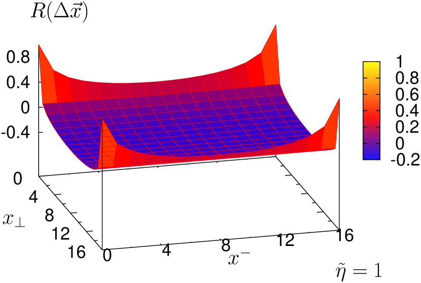
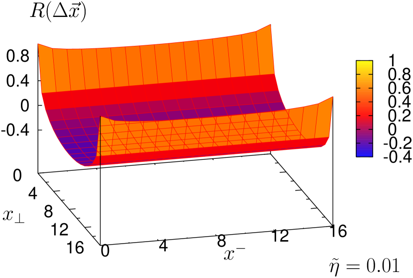
Figure 3: Ratio of covariance matrix elements $R(\Delta\vec{x})$ as a function of the separation $\Delta\vec{x}$ for a 2 dimensional $16\mathrm{x}16$ lattice at three different values of $\eta^{2}$.

For reasons of presentability, we have restricted ourselves to a $2$-dimensional section through the $3$-dimensional lattice spanned by $x_{\bot}=x^{1}$ and $x^{-}$ at $x^{2}=0$. This representation allows to see the anisotropy developing for very small $\tilde{\eta}$. Here and in the following, the notion “off-diagonal in position space” refers to $\Delta\vec{x}\neq 0$ whereas “diagonal in position space” refers to $\Delta\vec{x}=0$. For $\tilde{\eta}=1$, the covariance matrix has only weakly-off diagonal contributions in position space. Therefore, it is reasonable to consider the weak coupling wave functional in the diagonal approximation Chin:1985ua as a product of single plaquette functionals. For decreasing $\tilde{\eta}$ one observes that the correlations among plaquettes separated along the longitudinal direction become more and more important. In the light cone limit, every plaquette is equally correlated with any other plaquette which is longitudinally separated from the first one.

However, for not too small values of $\tilde{\eta}$, at least an effective description by a product of single plaquette wave functionals is possible. In Sec. VII we discuss a possibility to include long range correlations in the wave functional by a combined optimization and Quantum Diffusion Monte Carlo method.

VI Variational optimization of the ground state wave functional

In the last two sections we have analyzed the strong and weak coupling behavior of the Hamiltonian and its ground state. We have seen that in the strong coupling limit the ground state wave functional may be approximated by a product of single site wave functionals. Also in the weak coupling limit for not too small $\tilde{\eta}$ the bilocality of the chromo magnetic field strength is less important. In the following we construct an effective wave functional which smoothly interpolates between the strong and weak coupling solution. In addition we would like to choose the ground state wave functional in such a way that it is not invariant under the unwanted additional $Z(2)$ symmetry of the effective Hamiltonian in which the linear momentum terms are compensated by the translation operator. Therefore, me make a variational ansatz of the ground state wave functional for the whole coupling range which contains a product of single site plaquettes with two variational parameters $\rho$ and $\delta$. We denote the normalization constant by N

$$\Psi_{0}(\rho,\delta) = N\prod\limits_{\vec{x}}\exp\left\{\sum\limits_{k=1}^{2}\rho\,\mathrm{Tr}\left[\,\mathrm{Re}\Big{(}\,U_{-k}(\vec{x})\,\Big{)}\,\right]+\delta\,\mathrm{Tr}\left[\,\mathrm{Re}\Big{(}\,U_{12}(\vec{x})\,\Big{)}\,\right]\right\}\;.$$ (81)

With this normalized wave functional we variationally optimize the energy expectation value $\epsilon_{0}(\rho,\delta)$ of the effective Hamiltonian which is given in terms of plaquette expectation values.

$$\epsilon_{0}(\rho,\delta) = \left\langle\Psi_{0}\right|\mathcal{H}_{eff}\left|\Psi_{0}\right\rangle$$

$$= \phantom{+}\frac{1}{N_{-}N_{\bot}^{2}}\frac{1}{a_{\bot}^{4}}\frac{2}{\sqrt{\lambda}}\sum\limits_{\vec{x}\phantom{,k}}\left[\left(\frac{3}{4}\frac{\delta}{\tilde{\eta}^{2}}-\frac{\lambda}{2}\right)\left\langle\mathrm{Tr}\left[\,\mathrm{Re}\Big{(}\,U_{12}(\vec{x})\,\Big{)}\,\right]\right\rangle+\lambda\right]$$

$$+\frac{1}{N_{-}N_{\bot}^{2}}\frac{1}{a_{\bot}^{4}}\frac{2}{\sqrt{\lambda}}\sum\limits_{\vec{x},k}\left[\frac{3}{8}\rho\left(1+\frac{1}{\tilde{\eta}^{2}}\right)\left\langle\mathrm{Tr}\left[\,\mathrm{Re}\Big{(}\,U_{-k}(\vec{x})\,\Big{)}\,\right]\right\rangle\right]$$

$$+\frac{1}{N_{-}N_{\bot}^{2}}\frac{1}{a_{\bot}^{4}}\frac{2}{\sqrt{\lambda}}\sum\limits_{\vec{x},k}\left[\frac{\lambda}{2}\frac{1}{\tilde{\eta}^{2}}\left(1-\frac{1}{4}\left\langle\left(\mathrm{Tr}\left[\,\mathrm{Re}\Big{(}\,U_{-k}(\vec{x})\,\Big{)}\,\right]\right)^{2}\right\rangle\right)\right]\;.$$

The explicit dependence of the energy expectation value on $\rho$ and $\delta$ comes from the kinetic energy terms in $\mathcal{H}_{eff}$. There is an implicit dependence in the plaquette expectation values which are computed as averages over link configurations generated by the probability density

$$dP(U) = \left|\Psi_{0}(\rho,\delta)\right|^{2}\prod\limits_{\vec{x},j}\mathcal{D}U_{j}(\vec{x})~{}.$$ (83)

With the special form of our trial ground state wave functional Eq. (81), the energy expectation value of the effective Hamiltonian Eq. (46) coincides with the energy expectation value of the full Hamiltonian Eq. (42). Even if we do not use the invariance of the trial wave functional under translations, the expectation value of the longitudinal momentum operator with respect to the trial wave functional Eq. (81) vanishes identically. This is due to the fact that the expectation value of the chromo electric field operator $\Pi_{j}^{a}(\vec{y})$ times an arbitrary functional $G(\{U\})$ of the links with respect to a purely real valued exponential wave functional obeys

$$\left\langle\Psi_{0}\right|\Pi_{j}^{a}(\vec{y})~{}G(\{U\})\left|\Psi_{0}\right\rangle = -\left\langle\Psi_{0}\right|G(\{U\})~{}\Pi_{j}^{a}(\vec{y})\left|\Psi_{0}\right\rangle\;.$$ (84)

The above relation Eq. (84) may be interpreted as a “partial” integration rule and is proven in appendix A. Hence, the ground state wave functional Eq. (81) minimizing the energy density Eq. (LABEL:eqn:ExpValEnergyDens) optimizes simultaneously the effective and the full Hamiltonian. In order to optimize the ground state wave functional we sample the probability distribution Eq. (83) with a local heat bath algorithm Creutz:1980zw on a $16^{3}$-lattice and measure the expectation values of the plaquettes and the squared plaquettes with the bootstrap method Efron:1979 using an initial sample size of $500$ and a bootstrap sample size of $1000$. We compute these expectation values as a function of the parameters $\rho$ and $\delta$ on a $50\times 50$ grid where each of the parameters varies in the interval $[0,10]$ with a sterilize of $0.2$. This yields a set of $2500$ distinct expectation values which we interpolate with polynomials of fifth order. For a first coarse estimate of the optimized parameters, we find the minimum of Eq. (LABEL:eqn:ExpValEnergyDens) with a standard Mathematica minimization routine.

For the fine determination of the optimal parameters we then generate 50 different pairs with energy expectation values less than three percent higher than the energy at the coarse estimate of $\rho_{0},\delta_{0}$. Finally, we fit these energy values with a quadratic form Eq. (85) centered at the optimal values $(\rho_{0},\delta_{0})$ where the linear term in the taylor series vanishes due to the minimum condition

$$\epsilon_{0}(\rho,\delta)\approx\epsilon_{0}(\rho_{0},\delta_{0})+\frac{1}{2}\left(\begin{array}[]{c}\rho-\rho_{0}\\ \delta-\delta_{0}\end{array}\right)^{\mathrm{T}}\cdot\left(\begin{array}[]{cc}\frac{\partial^{2}\epsilon_{0}}{\partial_{\rho}\partial_{\rho}}&\frac{\partial^{2}\epsilon_{0}}{\partial_{\rho}\partial_{\delta}}\\ \frac{\partial^{2}\epsilon_{0}}{\partial_{\delta}\partial_{\rho}}&\frac{\partial^{2}\epsilon_{0}}{\partial_{\delta}\partial_{\delta}}\end{array}\right)\cdot\left(\begin{array}[]{c}\rho-\rho_{0}\\ \delta-\delta_{0}\end{array}\right)\;.$$ (85)

The described method is tested by comparing our results with the variational results of Chin et al. Chin:1985ua who optimized a one parameter ($2\,\rho=2\,\delta\equiv\alpha_{\mathrm{Chin}}$) wave functional of the form given in Eq. (81) with respect to the standard equal time Hamiltonian containing only plaquette terms without anisotropy. Note that Chin’s results have been obtained on a $4^{3}$-lattice, but the authors show that the dependence of the energy density and the optimal wave functional parameter on the lattice size is small. We find $0.5\%$ agreement between the results of our method and the values obtained by Chin et al. Chin:1985ua .

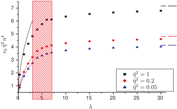
Figure 4: Optimized energy density as a function of $\lambda$ obtained from the simulation on a $16^{3}$ lattice for three different values of $\tilde{\eta}^{2}$. The red shaded area corresponds to the phase transition region for all values of $\tilde{\eta}^{2}$. The dotted lines show the predicted analytical strong coupling behavior. The arrows indicate the expected asymptotic behavior for weak coupling which is a constant independent of $\lambda$.

Next we apply the described optimization method to the nlc Hamiltonian. The optimized energy density is presented in Fig. 4 as a function of $\lambda$ for different values of $\tilde{\eta}^{2}$. The $1/\tilde{\eta}^{2}$ divergence is scaled out. The curve has a $\sqrt{\lambda}$ behavior for strong coupling and is independent of $\lambda$ for weak coupling as found in Sec. V

$$\epsilon_{0}|_{\text{strong coupling}} = \frac{1}{\tilde{\eta}^{2}}\frac{1}{a_{\bot}^{4}}\left(\frac{3}{2}+2~{}\tilde{\eta}^{2}\right)\sqrt{\lambda}$$

$$\epsilon_{0}|_{\text{weak coupling}} = \frac{1}{a_{\bot}^{4}}\frac{6}{\tilde{\eta}^{2}}\frac{1}{N_{-}N_{\bot}^{2}}$$

$$\sum\limits_{\vec{k}}\left[\tilde{\eta}^{2}\sin\left(\frac{k_{1}}{2}\right)^{2}+\tilde{\eta}^{2}\sin\left(\frac{k_{2}}{2}\right)^{2}+\sin\left(\frac{k_{-}}{2}\right)^{2}\right]^{1/2}\;.$$

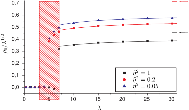
Figure 5: Optimal wave functional parameter $\rho_{0}(\lambda,\tilde{\eta})$ as a function of $\lambda$ obtained from the simulation on a $16^{3}$ lattice for three different values of $\tilde{\eta}^{2}$. The red shaded area corresponds to the phase transition region for all values of $\tilde{\eta}^{2}$. The dotted lines show the predicted analytical strong coupling behavior. The arrows indicate the expected asymptotic behavior for weak coupling which is proportional to $\sqrt{\lambda}$, i.e. a constant independent of $\lambda$ in the plot. The solid lines show the actual analytic parameterizations in the weak coupling regime (cf. Eq. (97)).

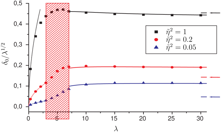
Figure 6: Optimal wave functional parameter $\delta_{0}(\lambda,\tilde{\eta})$ as a function of $\lambda$ obtained from the simulation on a $16^{3}$ lattice for three different values of $\tilde{\eta}^{2}$. The red shaded area corresponds to the phase transition region for all values of $\tilde{\eta}^{2}$. The dotted lines show the predicted analytical strong coupling behavior. The arrows indicate the expected asymptotic behavior for weak coupling which is proportional to $\sqrt{\lambda}$, i.e. a constant independent of $\lambda$ in the plot. The solid lines show the actual analytic parameterizations in the weak coupling regime (cf. Eq. (97)).

In Figs. 5 and 6, we present the variationally optimized wave functional parameters $\rho_{0}$ and $\delta_{0}$ as a function of $\lambda$ for different values of $\tilde{\eta}^{2}$. The parameters are divided by a factor $\sqrt{\lambda}$ such that they become constant in the weak coupling limit ($\lambda\rightarrow\infty$). The uncertainties on the variational parameters are typically $5\%$ and are larger in the region where the Hamiltonian with the adjoint plaquette in $(-k)$-direction induces a phase transition. Therefore, in principle only couplings in the weak coupling region above $\lambda=7$ are meaningful where the $Z(2)$ symmetry is spontaneously broken.

By using the strong coupling solution from Eq. (V.1) and the diagonal part of the covariance matrix at $\Delta\vec{x}=\vec{0}$ of the weak coupling solution Eq. (V.2), we get analytically the following estimates for $\rho_{0}$ and $\delta_{0}$

$$\rho_{0}(\lambda,\tilde{\eta}) = \left\{\begin{array}[]{lcr}0&\mathrm{for}&\lambda<<1\\ \sqrt{\lambda}~{}\gamma_{\tilde{\eta}}(\vec{0})\phantom{~{}\tilde{\eta}^{2}}&\mathrm{for}&\lambda>>1\end{array}\right.$$ (89)

$$\delta_{0}(\lambda,\tilde{\eta}) = \left\{\begin{array}[]{lcr}\frac{1}{3}~{}\lambda~{}\tilde{\eta}^{2}&\mathrm{for}&\lambda<<1\\ \sqrt{\lambda}~{}\tilde{\eta}^{2}~{}\gamma_{\tilde{\eta}}(\vec{0})&\mathrm{for}&\lambda>>1\end{array}\right.$$ (92)

$$\gamma_{\tilde{\eta}}(\vec{0}) \left\{\begin{array}[]{lcr}\sim 0.038/\tilde{\eta}&\mathrm{for}&\tilde{\eta}\rightarrow 0\\ =0.454&\mathrm{for}&\tilde{\eta}\rightarrow 1\end{array}\right.~{}.$$ (95)

The variationally determined parameters are in good agreement with the analytic predictions in the strong coupling regime. In the weak coupling regime the optimal parameters differ from the analytical estimates Eq. (95). In both cases the analytic predictions disagree more for small $\tilde{\eta}$. This is natural, since the light cone limit $\tilde{\eta}\rightarrow 0$ builds up correlations among plaquettes separated along the longitudinal direction. The parameters optimizing our product of single plaquette wave functionals effectively describe these correlations and adopt values which differ from the weak coupling estimate given by the diagonal entries of the covariance matrix Eq. (95).

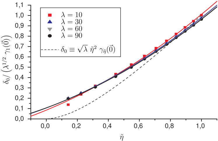
Figure 8: Optimal wave functional parameter $\delta_{0}(\lambda,\tilde{\eta})$ as a function of $\tilde{\eta}$ obtained from the simulation on a $16^{3}$ lattice for four different values of $\lambda$. The expected $\lambda^{1/2}~{}\gamma_{1}(\vec{0})$ behavior for the equal time Hamiltonian with $\tilde{\eta}=1$ is scaled out. The solid lines show the analytical parameterizations. The dotted line corresponds to the “naive” analytical weak coupling prediction.

In the following we analyze the $\tilde{\eta}$ dependence of the optimal wave functional parameters for fixed values of $\lambda$ which lie in the physical relevant region above $\lambda=7$. We show in Figs. 7 and 8 the optimal wave functional parameters $\rho_{0},\delta_{0}$ divided by $\sqrt{\lambda}~{}\gamma_{1}(\vec{0})$, i.e. $\sqrt{\lambda}~{}\gamma_{\tilde{\eta}}(\vec{0})$ for $\tilde{\eta}=1$, which is the expected behavior for the equal time Hamiltonian. This way we can show the variations of the wave functional parameters in the light cone limit. For a direct comparison, we plot the analytical weak coupling prediction Eq. (95) by dotted lines in the same figures. The analytical results for $\rho_{0}$ (Eq. (95)) overestimate the variationally determined values, whereas the analytical predictions for $\delta_{0}$ (Eq. (95)) underestimate the optimized parameters as a function of $\tilde{\eta}$. Here again, the large difference for small $\tilde{\eta}$ originates from the effective description of long range correlations by the parameters of our ground state wave functional in this parameter region. For sufficiently large values of $\lambda$, the $\tilde{\eta}$ behavior for $\rho_{0}$ and $\delta_{0}$ becomes universal and independent of $\lambda$. We determine functions $f_{\rho}$ and $f_{\delta}$ which describe the deviations of the variationally optimized wave functional parameters from the the weak coupling limit $\sqrt{\lambda}~{}\gamma_{1}(\vec{0})$ at $\tilde{\eta}=1$ (cf. Figs. 7 and 8)

$$\rho_{0}(\lambda,\tilde{\eta}) = \sqrt{\lambda}~{}\gamma_{1}(\vec{0})~{}f_{\rho}(\lambda,\tilde{\eta})$$

$$\delta_{0}(\lambda,\tilde{\eta}) = \sqrt{\lambda}~{}\gamma_{1}(\vec{0})~{}f_{\delta}(\lambda,\tilde{\eta})\;.$$ (96)

In the extreme weak coupling limit $\lambda\rightarrow\infty$ and close to $\tilde{\eta}\rightarrow 1$, each of the functions $f_{\rho}$ and $f_{\delta}$ may be described by linear functions of $\tilde{\eta}$. Therefore, it is reasonable to assume that $f_{\rho}$ and $f_{\delta}$ can be approximated by expansions around $\lambda\rightarrow\infty$ and $\tilde{\eta}=1$

$$f_{i}(\lambda,\tilde{\eta}) = c_{0,i}\left[1+\frac{c_{1,i}}{\lambda}+c_{2,i}~{}(1-\tilde{\eta})+\frac{c_{3,i}}{\lambda^{2}}+c_{4,i}~{}\frac{(1-\tilde{\eta})}{\lambda}+c_{5,i}~{}(1-\tilde{\eta})^{2}\right]$$

$$i = \rho,\delta\;.$$ (97)

The coefficients $c_{0,i}$ represent the effective single plaquette equal time wave functional parameters. A good fit of the parameters $c_{0,i},...,c_{5,i}$ minimizing $\chi^{2}$ in the range $\lambda\in[10,95]$ and $\tilde{\eta}\in[0.15,1]$ gives the coefficients tabulated in Table 1.

i	$c_{0,i}$	$c_{1,i}$	$c_{2,i}$	$c_{3,i}$	$c_{4,i}$	$c_{5,i}$
$\rho$	0.90	-1.74	0.72	4.06	-0.40	-0.14
$\delta$	0.95	0.93	-1.21	-3.22	-0.83	0.32

Table 1: Coefficients of Eq. (97) obtained from least square minimization.

This analytical parameterization of the ground state wave functional allows to smoothly interpolate between ground state wave functionals belonging to different coupling constants and different values of $\tilde{\eta}$ in the physical relevant coupling constant region. Furthermore, the given form induces generically a vanishing expectation value of $P_{-,lat}$ which makes it optimal for the use in a guided diffusion Monte Carlo as discussed in Sec. IV. Since it is an approximation to the exact ground state it may be used for further qualitative investigations: In a forthcoming paper we plan to determine hadronic cross sections by simulating how a color dipole moving along the light cone hits a neutral hadron localized at $x^{-}=0$. With the parameterization of Eq. (97) we are able to extrapolate the parameters of the wave functional to $\tilde{\eta}=0$

$$\rho_{0}(\lambda,0) = \left(0.65-\frac{0.87}{\lambda}+\frac{1.65}{\lambda^{2}}\right)\sqrt{\lambda}$$

$$\delta_{0}(\lambda,0) = \left(0.05+\frac{0.04}{\lambda}-\frac{1.39}{\lambda^{2}}\right)\sqrt{\lambda}\;.$$ (98)

At $\tilde{\eta}=0$, the color dipole can be represented by a longitudinal-transversal Wilson loop extended in $x^{-}$ direction and the simplified target can be modeled by a transverse plaquette. Varying the impact parameter one can sample the correlation function of the two gauge invariant objects and thereby obtain the profile function.

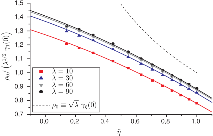
Figure 7: Optimal wave functional parameter $\rho_{0}(\lambda,\tilde{\eta})$ as a function of $\tilde{\eta}$ obtained from the simulation on a $16^{3}$ lattice for four different values of $\lambda$. The expected $\lambda^{1/2}~{}\gamma_{1}(\vec{0})$ behavior for the equal time Hamiltonian with $\tilde{\eta}=1$ is scaled out. The solid lines show the analytical parameterizations. The dotted line corresponds to the “naive” analytical weak coupling prediction.

VII Conclusions and outlook

Light cone coordinates are especially suited to parameterize high energy reactions for which perturbative QCD calculations have reached an unprecedented accuracy. In this paper we have addressed the question how to include non-perturbative features of QCD on the light cone. We propose to use lattice gauge theory formulated in exactly these coordinates.

We start from the standard lattice action written in terms of near light cone coordinates such that the continuum action is recovered in leading order in the lattice spacing. The distance to the light cone is tuned by the adjustment of an external parameter $\eta$. A transition to Euclidean time in this framework turns out to be problematic from a numerical point of view due to the fact that the Euclidean action remains complex which means that the integrand of the path integral cannot be interpreted as a probability measure anymore. Similar problems for QCD at finite baryonic density are generally referred to as the sign problem for which, up to the moment, no solution is known. In our case, this problem can be circumvented by applying the following strategy. We stay in Minkowski time, but switch to a Hamiltonian formulation of lattice gauge theory. Then the time evolution operator can be analytically continued to imaginary times and acts as a projector onto the exact ground state when it is applied to a trial state with a non-vanishing overlap with the exact ground state. Hence, instead of sampling the Euclidean path integral one manipulates a probability distribution for the product of the exact ground state wave functional and a guidance wave functional in a Quantum Diffusion Monte Carlo algorithm. For an improvement of the convergence of the diffusion Monte Carlo, the guidance wave functional should be sufficiently close to the exact ground state. The main goal of the present paper has been to develop a convenient and numerically realizable ground state projection operator and to propose such a guidance wave functional.

We first work out the more obvious continuum formulation. The continuum near light cone Hamiltonian has an asymmetry in the longitudinal and transversal fields. The transversal fields are “enhanced” in the Hamiltonian in comparison to the longitudinal ones by a factor of $1/\eta^{2}$ which is due to the underlying Lorentz transformation of the chromo magnetic and chromo electric fields. Furthermore, the obtained near light cone Hamiltonian is similar to the classical Hamiltonian of a charged particle moving in an electromagnetic background field, which contains terms linear in the particle momentum. Such terms yield complex branching ratios in a Quantum Monte Carlo algorithm which cannot be interpreted as probabilities and make it fail. However, this problem can be avoided. Linear terms in the QCD near light cone Hamilton operator can be compensated by the generator of longitudinal translations. The QCD ground state is translation invariant, i.e. an eigenstate of the longitudinal translation operator with zero eigenvalue. Since the Hamiltonian commutes with the longitudinal momentum operator, the longitudinal momentum is not affected by time evolution. Therefore, one is able to construct an effective Hamiltonian feasible for a Quantum Diffusion Monte Carlo having the same ground state as the exact Hamiltonian by adding the longitudinal momentum operator to the exact Hamiltonian.

Having checked feasibility in the continuum we derive the lattice Hamiltonian from the action via the transfer matrix method. We allow in general different lattice spacings in longitudinal and transversal directions. It is remarkable that the parameter $\eta$ controlling the distance to the light cone multiplies the lattice anisotropy parameter $\xi$ which represents the ratio of the longitudinal lattice spacing and the transversal lattice spacing. Since these two parameters always appear together, there is no difference between the light cone limit and the anisotropic lattice limit. We can construct an effective Hamiltonian similar to the continuum case by adding the effective longitudinal momentum operator to the lattice Hamiltonian.

We analytically compute the lattice ground state wave functional of the effective Hamiltonian in the strong and weak coupling limit. In the strong coupling limit we obtain a product of single plaquette wave functionals similar to the equal time scenario. In the weak coupling limit, the solution is equivalent to the solution of the near light cone Hamiltonian with abelian fields, i.e. it is a multivariate Gaussian wave functional with a covariance matrix weighting correlations of field strengths at different spatial separations.

Motivated by the strong and weak coupling solutions, we have constructed an effective ground state wave functional which smoothly interpolates between these two extreme results and which can be used as a guidance wave functional for a Quantum Diffusion Monte Carlo algorithm. It is a variational ansatz for the whole coupling range which contains a product of single plaquette wave functionals with two variational parameters. We have variationally optimized the parameters by minimizing the energy expectation value of the effective Hamiltonian with respect to the ground state wave functional. The effective ground state wave functional serves as a starting point for further qualitative explorations. It can also be extrapolated to $\tilde{\eta}=0$ and may be used to simulate correlation functions which appear in hadronic cross sections.

The effective ground state wave functional can be improved by allowing also long range correlations in the wave functional. This is motivated by the observation that in the weak coupling limit, the covariance matrix elements of the analytical ground state wave functional which connect longitudinally separated spatial points become more and more important. An exponential ansatz then may contain plaquettes which are connected back and forth via long strings of gauge links. In the light cone limit the energetically most favorable string configurations are elongated along the minus direction. Such an ansatz may interpolate in the whole coupling range by allowing a covariance matrix with adjustable parameters. Numerical techniques Beccaria:2000eg exist for a guided random walk in parameter space. So it may be possible to construct on the basis of an improved weak coupling solution a reasonable numerical procedure to obtain a good ground state for the effective lattice Hamiltonian.

There have been strong advances in light cone physics recently in string and supersymmetric theory Green:1987sp ; Green:1987mn . A careful study of near light cone theory in lattice QCD may supplement this successful work.

Appendix A Some useful commutator relations

In this section we collect some useful formulae for the computation of matrix elements. First, we want to apply an arbitrary kinetic energy operator to the unperturbed strong coupling ground state $\left|\Psi_{0}^{(0)}\right\rangle$ (cf. Sec. V.1) multiplied by an arbitrary function of the links

$$\sum\limits_{j,a,\vec{y}}c_{j}\Pi_{j}^{a}(\vec{y})^{2}f(\{U\})\left|\Psi_{0}^{(0)}\right\rangle = \sum\limits_{j,a,\vec{y}}c_{j}\left[\Pi_{j}^{a}(\vec{y})^{2},f(\{U\})\right]\left|\Psi_{0}^{(0)}\right\rangle$$ (99)

$$= \sum\limits_{j,a,\vec{y}}c_{j}\Pi_{j}^{a}(\vec{y})\left[\Pi_{j}^{a}(\vec{y}),f(\{U\})\right]\left|\Psi_{0}^{(0)}\right\rangle$$

$$= \sum\limits_{j,a,\vec{y}}c_{j}\left[\Pi_{j}^{a}(\vec{y}),\left[\Pi_{j}^{a}(\vec{y}),f(\{U\})\right]\right]\left|\Psi_{0}^{(0)}\right\rangle\;.$$

The following double commutators are of special interest

$$\sum\limits_{j,a,\vec{y}}c_{j}\left[\Pi_{j}^{a}(\vec{y}),\left[\Pi_{j}^{a}(\vec{y}),\mathrm{Tr}\left[\,\mathrm{Re}\Big{(}\,U_{kl}(\vec{x})\,\Big{)}\,\right]\right]\right]$$ (100)

$$= \frac{3}{2}\left(c_{k}+c_{l}\right)\mathrm{Tr}\left[\,\mathrm{Re}\Big{(}\,U_{kl}(\vec{x})\,\Big{)}\,\right]$$

and

$$\sum\limits_{j,a,\vec{y}}c_{j}\left[\Pi_{j}^{a}(\vec{y}),\left[\Pi_{j}^{a}(\vec{y}),\left(\mathrm{Tr}\left[\,~{}\mathrm{Re}\Big{(}\,U_{kl}(\vec{x})\,\Big{)}\,\right]\right)^{2}\right]\right]$$ (101)

$$= 4\left(c_{k}+c_{l}\right)\left[\left(\mathrm{Tr}\left[\,\mathrm{Re}\Big{(}\,U_{kl}(\vec{x})\,\Big{)}\,\right]\right)^{2}-1\right]\;.$$

For the elementary plaquette, we have the following commutation relation

$$\left[\widehat{\Pi}_{j}^{a}(\vec{y}),\mathrm{Tr}\left[\,\mathrm{Re}\Big{(}\,U_{kl}(\vec{x})\,\Big{)}\,\right]\right] = \phantom{-}\mathrm{i}\;\mathrm{Tr}\left[\,\frac{\sigma^{a}}{2}\;\mathrm{Im}\Big{(}\,U_{kl}(\vec{x})\,\Big{)}\,\right]\delta_{\vec{y},\vec{x}}\delta_{jk}$$ (102)

$$+\mathrm{i}\;\mathrm{Tr}\left[\,\frac{\sigma^{a}}{2}\;\mathrm{Im}\Big{(}\,U_{k}^{\dagger}(\vec{x})U_{kl}(\vec{x})U_{k}(\vec{x})\,\Big{)}\,\right]\delta_{\vec{y},\vec{x}+\vec{e}_{k}}\delta_{jl}$$

$$-\mathrm{i}\;\mathrm{Tr}\left[\,\frac{\sigma^{a}}{2}\;\mathrm{Im}\Big{(}\,U_{l}^{\dagger}(\vec{x})U_{kl}(\vec{x})U_{l}(\vec{x})\,\Big{)}\,\right]\delta_{\vec{y},\vec{x}+\vec{e}_{l}}\delta_{jk}$$

$$-\mathrm{i}\;\mathrm{Tr}\left[\,\frac{\sigma^{a}}{2}\;\mathrm{Im}\Big{(}\,U_{kl}(\vec{x})\,\Big{)}\,\right]\delta_{\vec{y},\vec{x}}\delta_{jl}\;.$$

In the following we assume an exponential ground state wave functional with exponent $F(\{U\})$ where $F(\{U\})$ is some arbitrary real valued functional of the links and $\left|\Psi_{0}^{(0)}\right\rangle$ is the unperturbed strong coupling ground state (cf. Sec. V.1)

$$\Big{|}\Psi_{0}\Big{\rangle} = \exp\left[F(\{U\})\right]\left|\Psi_{0}^{(0)}\right\rangle$$

$$\Rightarrow\Big{\langle}\Psi_{0}\Big{|} = \left\langle\Psi_{0}^{(0)}\right|\exp\left[F(\{U\})\right]~{}.$$ (103)

Then, the expectation value of the color trace of the momentum operator $\Pi_{j}^{a}(\vec{y})$ squared with respect to the ground state Eq. (103) is given by

$$\sum\limits_{j,a,\vec{y}}c_{j}\left\langle\Psi_{0}\right|\Pi_{j}^{a}(\vec{y})^{2}\left|\Psi_{0}\right\rangle=$$ (104)

$$\sum\limits_{j,a,\vec{y}}c_{j}\left\langle\Psi_{0}\right|\frac{1}{2}\left[\Pi_{j}^{a}(\vec{y}),\left[\Pi_{j}^{a}(\vec{y}),F(U)\right]\right]\left|\Psi_{0}\right\rangle~{}.$$

The expectation value of the momentum operator $\Pi_{j}^{a}(\vec{y})$ times an arbitrary functional $G(\{U\})$ of the links is given by

$$\Big{\langle}\Psi_{0}\Big{|}\Pi_{j}^{a}(\vec{y})~{}G(\{U\})\Big{|}\Psi_{0}\Big{\rangle} = \phantom{-}\Big{\langle}\Psi_{0}^{(0)}\Big{|}\exp\Big{[}F(\{U\})\Big{]}~{}\Pi_{j}^{a}(\vec{y})~{}G(\{U\})$$ (105)

$$~{}~{}~{}~{}~{}~{}~{}~{}~{}~{}~{}~{}~{}~{}~{}~{}~{}~{}~{}~{}~{}~{}~{}~{}\cdot\exp\Big{[}F(\{U\})\Big{]}\Big{|}\Psi_{0}^{(0)}\Big{\rangle}$$

$$= -\Big{\langle}\Psi_{0}^{(0)}\Big{|}\left[\Pi_{j}^{a}(\vec{y}),\exp\Big{[}F(\{U\})\Big{]}\right]~{}~{}G(\{U\})$$

$$~{}~{}~{}~{}~{}~{}~{}~{}~{}~{}~{}~{}~{}~{}~{}~{}~{}~{}~{}~{}~{}~{}~{}~{}\cdot\exp\Big{[}F(\{U\})\Big{]}\Big{|}\Psi_{0}^{(0)}\Big{\rangle}$$

$$= -\Big{\langle}\Psi_{0}^{(0)}\Big{|}\exp\Big{[}F(\{U\})\Big{]}~{}G(\{U\})$$

$$~{}~{}~{}~{}~{}~{}~{}~{}~{}~{}~{}~{}\cdot\left[\Pi_{j}^{a}(\vec{y}),\exp\Big{[}F(\{U\})\Big{]}\right]\Big{|}\Psi_{0}^{(0)}\Big{\rangle}$$

$$= -\Big{\langle}\Psi_{0}^{(0)}\Big{|}\exp\Big{[}F(\{U\})\Big{]}~{}G(\{U\})~{}\Pi_{j}^{a}(\vec{y})$$

$$~{}~{}~{}~{}~{}~{}~{}~{}~{}~{}~{}~{}~{}~{}~{}~{}~{}~{}~{}~{}~{}~{}~{}~{}\cdot\exp\Big{[}F(\{U\})\Big{]}\Big{|}\Psi_{0}^{(0)}\Big{\rangle}$$

$$= -\Big{\langle}\Psi_{0}\Big{|}G(\{U\})~{}\Pi_{j}^{a}(\vec{y})\Big{|}\Psi_{0}\Big{\rangle}\;.$$

Appendix B Derivation of the transfer matrix operator T

In this appendix we construct the transfer matrix operator $\mathbf{T}$ propagating a spatial lattice configuration from one time slice to the next and the Hilbert space on which it acts. Operators are written explicitly in boldface. The Hilbert space on which $\mathbf{T}$ operates contains general states $\left|\Psi\right\rangle$ which can be expanded in link states:

$$\left|\Psi\right\rangle=\int\mathcal{D}\mathcal{U}\;\Psi(\mathcal{U})\left|\mathcal{U}\right\rangle\;.$$ (106)

The measure is $\mathcal{D}\mathcal{U}$ in Eq. (106) refers to the correspondent product of $SU(2)$ Haar measures

$$\mathcal{D}\mathcal{U} = \prod\limits_{\vec{x},j}dU_{j}\left(\vec{x}\right)\;.$$ (107)

The inner product in this Hilbert space is given by

$$\left\langle\Psi^{\prime}\right|\left.\Psi\right\rangle=\int\mathcal{D}\mathcal{U}\;\Psi^{\prime}(\mathcal{U})^{*}\;\Psi(\mathcal{U})\;.$$ (108)

We define the operator $\mathbf{T}$ such that its matrix elements in the link basis are given by the transfer matrix Eq. (36)

$$\left\langle\mathcal{U}(x^{\prime+})\right|\mathbf{T}\Big{|}\mathcal{U}(x^{+})\Big{\rangle}\equiv T(x^{\prime+},x^{+})\;.$$ (109)

The path integral for finite lattice of $N_{\tau}$ time slices with periodic boundary conditions can be written as the trace of the $N_{\tau}$-fold product of transfer matrices

$$\int\prod\limits_{x}\prod\limits_{j=1,2,-}dU_{j}(x)e^{\mathrm{i}S_{lat}}=\mathrm{Tr}\left[\,\mathbf{T}^{N_{\tau}}\,\right]\;.$$ (110)

The transfer-matrix operator $\mathbf{T}$ is related to the Hamiltonian, the generator of time translations

$$\mathbf{T}=e^{-\mathrm{i}a_{+}\mathbf{H}}\hskip 14.22636pt\Rightarrow\hskip 14.22636pt\mathbf{H}=\lim_{a_{+}\rightarrow 0}-\frac{1}{\mathrm{i}a_{+}}\log\left(\mathbf{T}\right)\;.$$ (111)

We define with the group elements $g_{j}(\vec{x})\in SU(2)$ the following operators

$$\mathbf{U}_{j}(\vec{x})\left|\mathcal{U}\right\rangle = U_{j}(\vec{x})\left|\mathcal{U}\right\rangle~{}~{}~{}~{}\forall j,\vec{x}$$

$$\mathbf{R}\Bigl{(}g_{j}(\vec{x})\Bigr{)}\left|\mathcal{U}\right\rangle = \left|\mathcal{U}^{\prime}\right\rangle$$

$$\left|\mathcal{U}^{\prime}\right\rangle = \left|\ldots,g_{j}(\vec{x})U_{j}(\vec{x}),\ldots\right\rangle\;.$$ (112)

Here all links in $\left|\mathcal{U}^{\prime}\right\rangle$ coincide with the correspondent links in $\left|\mathcal{U}\right\rangle$ except for the link $U_{j}(\vec{x})$ which is left multiplied by $g_{j}(\vec{x})$. The operator $\mathbf{R}(g_{j}(\vec{x}))$ is similar to the translation operator in Quantum Mechanics. It is a unitary operator and satisfies the group representation property, i.e.

$$\mathbf{R}\Bigl{(}g_{j}(\vec{x})\Bigr{)}\mathbf{R}\Bigl{(}g_{j}^{\prime}(\vec{x})\Bigr{)}=\mathbf{R}\Bigl{(}g_{j}(\vec{x})\cdot g_{j}^{\prime}(\vec{x})\Bigr{)}\;.$$ (113)

The group elements $g_{j}(\vec{x})$ are parameterized by the exponential map which yields the Haar measure $dg_{j}(\vec{x})$

$$g_{j}(\vec{x}) = e^{\mathrm{i}\gamma_{j}^{a}(\vec{x})\sigma^{a}/2}~{},~{}\gamma_{j}^{a}(\vec{x})\in\mathrm{reals}$$

$$dg_{j}(\vec{x}) = J\Bigl{(}\vec{\gamma}_{j}(\vec{x})\Bigr{)}\prod\limits_{a}d\gamma_{j}^{a}(\vec{x})\;.$$ (114)

The Jacobian $J$ is equal to unity in a neighborhood of $\vec{\gamma}_{j}(\vec{x})=\vec{0}$. Introducing the momentum operators $\mathbf{\Pi}_{j}^{a}(\vec{x})$ canonically conjugate to $\mathbf{U}_{j}(\vec{x})$ we have

$$\mathbf{R}\Bigl{(}g_{j}(\vec{x})\Bigr{)} = e^{-\mathrm{i}\gamma_{j}^{a}(\vec{x})\mathbf{\Pi}_{j}^{a}(\vec{x})}$$

$$g_{j}(\vec{x}) = e^{\mathrm{i}\gamma_{j}^{a}(\vec{x})\sigma^{a}/2}$$

$$\left[\mathbf{\Pi}_{j}^{a}(\vec{x}),\mathbf{U}_{j^{\prime}}(\vec{x}^{\prime})\right] = \phantom{-}\frac{\sigma_{a}}{2}~{}\mathbf{U}_{j}(\vec{x})~{}\delta_{j,j^{\prime}}~{}\delta_{\vec{x},\vec{x}^{\prime}}\;,$$

$$\left[\mathbf{\Pi}_{j}^{a}(\vec{x}),\mathbf{U}_{j^{\prime}}^{\dagger}(\vec{x}^{\prime})\right] = -\mathbf{U}_{j}^{\dagger}(\vec{x})~{}\frac{\sigma_{a}}{2}~{}\delta_{j,j^{\prime}}~{}\delta_{\vec{x},\vec{x}^{\prime}}\;.$$ (115)

In contrast to the continuum commutation relations Eq. (22), the lattice momentum operators canonically conjugate to $\mathbf{U}_{j}(\vec{x})$ do not commute.

$$\left[\left[\mathbf{\Pi}_{j}^{a}(\vec{x}),\mathbf{\Pi}_{j^{\prime}}^{b}(\vec{x}^{\prime})\right],\mathbf{U}_{k}(\vec{y})\right] = \left[\left[\frac{\sigma^{a}}{2},~{}\frac{\sigma^{b}}{2}\right]~{},\mathbf{U}_{k}(\vec{y})\right]~{}\delta_{j,k}~{}\delta_{\vec{x},\vec{y}}~{}\delta_{j^{\prime},k}~{}\delta_{\vec{x}^{\prime},\vec{y}}$$ (116)

$$= \mathrm{i}~{}\epsilon^{abc}~{}\left[\frac{\sigma^{c}}{2},~{}\mathbf{U}_{k}(\vec{y})\right]~{}\delta_{j,j^{\prime}}~{}\delta_{\vec{x},\vec{x}^{\prime}}~{}\delta_{j,k}~{}\delta_{\vec{x},\vec{y}}$$

$$= \mathrm{i}~{}\epsilon^{abc}~{}\left[\mathbf{\Pi}_{j}^{c}(\vec{x}),~{}\mathbf{U}_{k}(\vec{y})\right]~{}\delta_{j,j^{\prime}}~{}\delta_{\vec{x},\vec{x}^{\prime}}\;.$$

Since this relation is true for arbitrary $\mathbf{U}_{k}(\vec{y})$, we get

$$\left[\mathbf{\Pi}_{j}^{a}(\vec{x}),\mathbf{\Pi}_{j^{\prime}}^{b}(\vec{x}^{\prime})\right] = \mathrm{i}~{}\varepsilon^{abc}~{}\mathbf{\Pi}_{j}^{c}(\vec{x})~{}\delta_{j,j^{\prime}}~{}\delta_{\vec{x},\vec{x}^{\prime}}\;,$$ (117)

$$\left[\mathbf{\Pi}_{j}(\vec{x})^{2},\mathbf{\Pi}_{j^{\prime}}^{b}(\vec{x}^{\prime})\right] = 0\;.$$ (118)

Note that we have defined the translation operator on the group manifold $\mathbf{R}$ with an opposite sign inside of the exponential in comparison with creutz . Our definition yields the same commutation relations as Kogut:1974ag which reproduce the continuum commutation relations Eq. (22) with the gauge field $A_{j}^{a}(\vec{x})$ in the naive continuum limit. For simplicity we abandon to write quantum mechanical operators explicitly in boldface in the following. By using the group translation operators $R$ we may write for the transfer matrix operator

$${T} = \Bigg{[}\Bigg{[}\prod\limits_{\vec{x}}\int dg_{-}(\vec{x})~{}{R}\Bigl{(}g_{-}(\vec{x})\Bigr{)}~{}\exp\left\{\mathrm{i}\frac{2}{g^{2}}~{}\frac{a_{\bot}^{2}}{a_{+}a_{-}}~{}\mathrm{Tr}\left[\,\mathds{1}-\mathrm{Re}\Big{(}\,g_{-}(\vec{x}\,\Big{)}\,\right]\right\}\Bigg{]}\Bigg{]}\times$$

$$\Bigg{[}\Bigg{[}\prod\limits_{\vec{x},k}\int dg_{k}(\vec{x})~{}{R}\Bigl{(}g_{k}(\vec{x})\Bigr{)}~{}\exp\left\{\mathrm{i}~{}\frac{2}{g^{2}}~{}\eta^{2}~{}\frac{a_{-}}{a_{+}}~{}\mathrm{Tr}\left[\,\mathds{1}-\mathrm{Re}\Big{(}\,g_{k}(\vec{x})\,\Big{)}\,\right]\right\}\Bigg{.}\Bigg{.}$$

$$\Bigg{.}\Bigg{.}\hskip 28.45274pt\times~{}\exp\left\{\mathrm{i}~{}\frac{2}{g^{2}}~{}\mathrm{Tr}\left[\,\mathrm{Im}\Big{(}\,g_{k}(\vec{x})\,\Big{)}~{}\mathrm{Im}\Big{(}\,{U}_{-k}(\vec{x})\,\Big{)}\,\right]\right\}\Bigg{]}\Bigg{]}\times$$

$$\Bigg{[}\Bigg{[}\prod\limits_{\vec{x}}\exp\left\{-\mathrm{i}~{}\frac{2}{g^{2}}~{}\frac{a_{+}a_{-}}{a_{\bot}^{2}}~{}\mathrm{Tr}\left[\,\mathds{1}-\mathrm{Re}\Big{(}\,{U}_{12}(\vec{x})\,\Big{)}\,\right]\right\}\Bigg{]}\Bigg{]}\;.$$

It still has the right matrix elements Eq. (109). In order to arrive at Eq. (B) one uses the fact that $R(g_{j}(\vec{x}))$ parameterizes the translation in group space from $U_{j}(\vec{x},x^{+})\rightarrow U_{j}(\vec{x},x^{\prime+})$

$$g_{j}(\vec{x})=U_{j}(\vec{x},x^{\prime+})U_{j}^{\dagger}(\vec{x},x^{+})\;.$$ (120)

Now, one may perform the group integrations in Eq. (B) explicitly. In the limit $a_{+}\rightarrow 0$, the time evolution along one temporal step $a_{+}$ induces rotations $g_{j}(\vec{x})$ which are of the order $a_{+}$ and are close to $\mathds{1}$. This implies that the parameters $\gamma_{j}^{a}(\vec{x})$ parameterizing these shifts are of the order $a_{+}$ as well. Therefore, it is convenient to make an expansion around $\gamma_{j}^{a}(\vec{x})=0$ up to order $\mathcal{O}(a_{+}^{2})$. In this limit, the Jacobian is approximately equal to $1$ and the integrals become Gaussian integrals which can be analytically computed. One obtains

$${H}_{\mathrm{lat}} = \lim_{a_{+}\rightarrow 0}\left[-\frac{1}{\mathrm{i}a_{+}}\log\left(T\right)\right]$$

$$= \sum\limits_{\vec{x}}\Bigg{[}\Bigg{[}~{}\frac{g^{2}}{2}~{}\frac{1}{a_{-}}~{}\sum\limits_{k,a}~{}\frac{1}{\eta^{2}}~{}\left\{~{}{\Pi}_{k}^{a}(\vec{x})-\frac{2}{g^{2}}~{}\mathrm{Tr}\left[\,\frac{\sigma_{a}}{2}~{}\mathrm{Im}\Big{(}\,{U}_{-k}(\vec{x})\,\Big{)}\,\right]\right\}^{2}\Bigg{.}\Bigg{.}$$

$$\hskip 14.22636pt\Bigg{.}\Bigg{.}+~{}\frac{g^{2}}{2}~{}\frac{a_{-}}{a_{\bot}^{2}}~{}\sum\limits_{a}{\Pi}_{-}^{a}(\vec{x})^{2}+~{}\frac{2}{g^{2}}~{}\frac{a_{-}}{a_{\bot}^{2}}~{}\mathrm{Tr}\left[\,\mathds{1}-\mathrm{Re}\Big{(}\,{U}_{12}(\vec{x})\,\Big{)}\,\right]\Bigg{]}\Bigg{]}\;.$$

References

• (1)
• (2) K. G. Wilson, Phys. Rev. D10 (1974) 2445.
• (3) M. Creutz, Phys. Rev. Lett. 43, (1979) 553.
• (4) C. Feuchter and H. Reinhardt, Phys. Rev.  D 70 (2004) 105021 [arXiv:hep-th/0408236].
• (5) R. G. Leigh, D. Minic and A. Yelnikov, Phys. Rev. Lett.  96 (2006) 222001 [arXiv:hep-th/0512111].
• (6) J. Greensite and S. Olejnik, arXiv:0707.2860 [hep-lat].
• (7) D. Mustaki, Phys. Rev.  D 38 (1988) 1260.
• (8) W. A. Bardeen, R. B. Pearson and E. Rabinovici, Phys. Rev.  D 21 (1980) 1037.
• (9) M. Burkardt and S. Dalley, Prog. Part. Nucl. Phys.  48 (2002) 317 [arXiv:hep-ph/0112007].
• (10) S. Dalley, IPPP-03-71 Proceedings of Light-Cone Workshop: Hadrons and Beyond (LC 03), Durham, England, 5-9 Aug 2003.
• (11) S. J. Brodsky, H. C. Pauli and S. S. Pinsky, Phys. Rept.  301 (1998) 299 [arXiv:hep-ph/9705477].
• (12) F. Lenz, K. Ohta, M. Thies and K. Yazaki, Phys. Rev. D 70 (2004) 025015 [arXiv:hep-th/0403186].
• (13) S. Dalley and B. van de Sande, arXiv:hep-ph/0311368.
• (14) G. Mack, Nucl. Phys. B 235 (1984) 197.
• (15) H. J. Pirner, Prog. Part. Nucl. Phys.  29 (1992) 33.
• (16) S. Dalley and B. van de Sande, Phys. Rev. D 67 (2003) 114507 [arXiv:hep-ph/0212086].
• (17) E. V. Prokhvatilov, H. W. L. Naus and H. J. Pirner, Phys. Rev. D 51 (1995) 2933 [arXiv:hep-ph/9406275].
• (18) H. W. L. Naus, H. J. Pirner, T. J. Fields and J. P. Vary, Phys. Rev. D 56 (1997) 8062 [arXiv:hep-th/9704135].
• (19) E. M. Ilgenfritz, Y. P. Ivanov and H. J. Pirner, Phys. Rev. D 62 (2000) 054006 [arXiv:hep-ph/0003005].
• (20) F. Lenz, H. W. L. Naus and M. Thies, Annals Phys.  233 (1994) 317.
• (21) H. Verlinde and E. Verlinde, arXiv:hep-th/9302104.
• (22) I. Y. Arefeva, Phys. Lett. B 328 (1994) 411 [arXiv:hep-th/9306014].
• (23) J. Raufeisen and S. J. Brodsky, Phys. Rev.  D 70 (2004) 085017 [arXiv:hep-th/0408108].
• (24) E. V. Prokhvatilov and V. A. Franke, Sov. J. Nucl. Phys.  49 (1989) 688 [Yad. Fiz.  49 (1989) 1109].
• (25) F. Lenz, M. Thies, K. Yazaki and S. Levit, Annals Phys.  208 (1991) 1.
• (26) E. Iancu, A. Leonidov and L. McLerran, arXiv:hep-ph/0202270.
• (27) A. Babansky and I. Balitsky, Phys. Rev.  D 67 (2003) 054026 [arXiv:hep-ph/0212075].
• (28) S. A. Chin, J. W. Negele and S. E. Koonin, Annals Phys.  157 (1984) 140.
• (29) S. A. Chin, O. S. Van Roosmalen, E. A. Umland and S. E. Koonin, Phys. Rev. D 31 (1985) 3201.
• (30) D. W. Heys and D. R. Stump, Phys. Rev.  D 30 (1984) 1315.
• (31) D. M. Ceperley and M. H. Kalos, in Monte Carlo Methods in Statistical Mechanics, edited by K. Binder (Springer-Verlag, New York, 1979).
• (32) C. J. Hamer, M. Samaras and R. J. Bursill, Phys. Rev.  D 62 (2000) 074506 [arXiv:hep-lat/0005009].
• (33) E. M. Ilgenfritz, S. A. Paston, H. J. Pirner, E. V. Prokhvatilov and V. A. Franke, Theor. Math. Phys.  148 (2006) 948 [Teor. Mat. Fiz.  148 (2006) 89].
• (34) M. Creutz, Phys. Rev. D 15 (1977) 1128.
• (35) J. B. Kogut and L. Susskind, Phys. Rev. D 11 (1975) 395.
• (36) C. J. Hamer and W. H. Zheng, Phys. Rev. D 48 (1993) 4435.
• (37) M. Creutz, Phys. Rev.  D 21 (1980) 2308.
• (38) B. Efron, The Annals of Statistics 7 (1979) 1.
• (39) M. Beccaria, Phys. Rev.  D 62 (2000) 034510 [arXiv:hep-lat/0003016].
• (40) M. B. Green, J. H. Schwarz and E. Witten, “SUPERSTRING THEORY. VOL. 1: INTRODUCTION,” Cambridge, Uk: Univ. Pr. ( 1987) 469 P. ( Cambridge Monographs On Mathematical Physics).
• (41) M. B. Green, J. H. Schwarz and E. Witten, “Superstring Theory. Vol. 2: Loop Amplitudes, Anomalies And Phenomenology,” Cambridge, Uk: Univ. Pr. ( 1987) 596 P. ( Cambridge Monographs On Mathematical Physics).