Neutrinos from Fallback onto Newly Formed Neutron Stars

Abstract

In the standard supernova picture, type Ib/c and type II supernovae are powered by the potential energy released in the collapse of the core of a massive star. In studying supernovae, we primarily focus on the ejecta that makes it beyond the potential well of the collapsed core. But, as we shall show in this paper, in most supernova explosions, a tenth of a solar mass or more of the ejecta is decelerated enough that it does not escape the potential well of that compact object. This material falls back onto the proto-neutron star within the first 10-15 seconds after the launch of the explosion, releasing more than $10^{52}$ erg of additional potential energy. Most of this energy is emitted in the form of neutrinos and we must understand this fallback neutrino emission if we are to use neutrino observations to study the behavior of matter at high densities. Here we present both a 1-dimensional study of fallback using energy-injected, supernova explosions and a first study of neutrino emission from fallback using a suite of 2-dimensional simulations.

1 Introduction

The collapse of a massive star down to a neutron star releases over $10^{53}$ erg of potential energy. Just one percent of this energy is required to power the observed type Ib/c and type II supernovae. Most of the energy is emitted in the form of neutrinos. How this small fraction of the energy is converted into explosion energy is still a matter of debate, but it is believed by most that neutrinos play a role in depositing energy above the collapsed core to drive this explosion (see Fryer 2003 for a review). Whether or not neutrinos are important for the explosion, they do provide astronomers a window into the explosion mechanism behind supernovae.

Neutrinos also provide a window into the material conditions at the core of a supernova explosion. With temperatures above 10 MeV and densities above nuclear densities, core-collapse supernovae make ideal laboratories for nuclear physics. To extract information about nuclear physics from such laboratories, we must understand the systematics in our supernova experiment. When the explosion engine is active, convective motions in the engine (Herant et al. 1994) make it very difficult to interpret the neutrino signal. An observed elevated neutrino luminosity could be a change in the neutrino opacity or it could be a difference in the convective engine. One approach to eliminate issues with convection would be to wait until all convective activity ceases. A number of studies have now been presented following the evolution of a collapsing star over 0.5-1.5 s after bounce (Fryer & Heger 2000; Burrows et al. 2006; Scheck et al. 2006; and, in 3-dimensions, Fryer & Young 2007). In all these calculations, hydrodynamic motions near the proto-neutron star continue to dramatically affect the neutrino emission through the end of the simulations. To achieve a clean neutrino signal, we must wait until after the launch of the explosion. We must also wait a few seconds after the launch of the explosion because the proto-neutron star may experience deep convection (Keil et al. 1996). After this time (roughly a few seconds to 10-20 s), the supernova finally seems to have achieved an ideal condition as a physics laboratory (Reddy et al. 1999). After 10-20 s, the neutrino signal will be too weak to do much experimental science, so we truly are limited to this narrow time window.

Unfortunately, even at these late times, Nature does not allow completely pristine conditions. Material falling back from the supernova explosion (“fallback”) may well produce a new round of convection and confusion to our neutrino signal. This fallback has been studied both in its important role in calculating the initial mass of the neutron star formed in a supernova explosion (e.g. Fryer & Kalogera 2001) and in estimating the r-rpocess yields in supernovae Fryer et al. (2006). In this paper, we study its role in determining the neutrino luminosity arising after the first few seconds of a supernova. In §2, we review the history of supernova fallback and present new calculations of supernova explosions estimating the fallback for a range of explosion energies and stellar masses. §3 describes the 2-dimensional code used to model the neutrino emission from the this fallback and shows results for the suite of simulations run for this paper. Different than the multi-dimensional simulations modeling stellar collapse, these simulations do not start at the onset of collapse (or bounce) and end at the launch of the explosion. Instead, they start a 2-10 s (depending on the explosion energy, etc. from §2) after the launch of the explosion when material begins to fall back onto the neutron star. We conclude with a brief discussion on how neutrino signals can be used to help better understand the supernova explosion, neutron star birth masses and neutrino cross-sections.

2 Supernova Fallback

The idea of fallback was first discussed by Colgate (1971) to overcome nucleosynthesis issues arising from the supernova ejection of neutron rich material produced in stellar cores (Arnett 1971, Young et al. 2006). Colgate argued that the inner layers of the ejected material would deposit its energy to the stellar material above it, ultimately reducing its energy below that needed to escape the neutron star, and it would fall back onto the neutron star. In such a scenario, one would expect the inner material to fall back quickly (within the first few to ten seconds). It was argued that this material (the neutron rich material from the initial explosion) would accrete onto the neutron star, alleviating any nucleosynthesis issues.

Since this work by Colgate, supernova explosion calculations have confirmed that fallback does occur (Bisnovatyi-Kogan & Lamzin 1984; Woosley 1989; Fryer et al. 1999; MacFadyen et al. 2001) and new arguments for the cause of this fallback were suggested. For example, Woosley (1989) argued that when the supernova shock decelerates in the hydrogen layers of the star, it sends a reverse shock that drives fallback. Such a model argues that the fallback will happen at late times, long after it can affect the neutrino luminosity from the cooling proto-neutron star. It also suggested that close binary systems (where a star’s hydrogen envelope was removed prior its collapse) might experience a very different amount of fallback than the amount of fallback in the collapse of a single star.

Which is the true cause of the fallback? And more to the point for neutrino emission, when does fallback occur? This confusion has mostly exists because, without a quantitatively reliable explosion mechanism, scientists have artificially driven supernova explosions to be able to study the results of these explosions (e.g. supernova light curves, nucleosynthetic yields, and fallback). Much of the past work (e.g. Woosley 1989; Fryer et al. 1999; MacFadyen et al. 2001) used piston driven explosions. By moving the piston out, scientists artificially lowered the amount of fallback and delayed this fallback considerably. These calculations all predicted that fallback would occur more than 100 s after the launch of the explosion.

But the piston-driven explosion mechanism may not accurately model the nature of the fallback. Young & Fryer (2007) found that piston-driven explosions produced both different fallback rates and different nucleosynthetic yields than energy-driven explosions of the same final energy. The errors in the yields or light-curves are on par with slight changes in the explosion energy. Such small errors seemed unimportant in matching the observations. For fallback, the differences are much more dramatic. Not only does the amount of fallback change, but the timescale at which the fallback occurs can change by more than an order of magnitude, moving a falback time of a few hundred seconds down to just 3-15 s. This changes the fallback accretion rate by over an order of magnitude and ultimately determines whether or not fallback is important in estimating the observed neutrino signal. It also means that the the amount of fallback will not change between binary and single stars (unless binary interactions change the internal structure of the star).

In this paper, we focus on fallback calculations from energy-injected explosions. Energy-injection is much better at mimicking the currently-favored supernova mechnanisms. Let’s take the convection-enhanced, neutrino-driven supernova engine as an example (see Fryer 2003 for a review). In this mechanism, the basic energy source is neutrinos (either diffusing out of the proto-neutron star core or from newly accreting material) that heat the atmosphere above the neutron star. This atmosphere is topped by the accretion shock of the infalling star. When enough energy is deposited in this region, the accretion shock will be pushed outward and an explosion occurs. Convection aids this mechanism by both allowing heated material to rise (cooling by adiabatic expansion instead of forcing it to continue to heat until it can cool by neutrino emission) and allowing shocked material at the top of the convective region to flow down to the neutron star surface to accrete onto the neutron star (emitting neutrinos) or be heating to be part of the rising bubble.

An energy injection method, although not mimicking the effects of convection directly, can mimick the basic tenets of this model - heating just above the neutron star surface to blow off the accretion shock. Ideally, once the region above the neutron star becomes more rarefied, the energy injection will essentially halt (aside from a weak, by supernova standards, neutrino-driven wind). Some groups have gone so far as to only inject this energy through a neutrino flux (Frölich et al. 2006). In this manner, once the region becomes rarefied, the energy injection drops naturally. A piston-driven explosion can not mimic this effect well unless very specific attention is paid to the input of the piston. The very different fallback results from piston explosions demonstrate just how far off such explosions are from the energy drive of the standard neutrino model.

This does not mean that by using energy-injection, we can produce a definitive fallback estimate for a supernova explosion. The explosion energy is one of our primary uncertainties in estimating the fallback rate. Supernova scientists have yet to agree on the exact mechanism behind the supernovae and we are far from achieving quantitative predictions of these explosions. With accurate light-curve and spectra calculations, we may be able to estimate the explosion energy for a particular supernova based on its observations. By studying a range of explosion energies for a given progenitor, we can provide a template for the neutrino flux (from fallback) arising from these systems, allowing us to possibly extract this effect and once more focus a study on the physics of dense, hot matter.

2.1 Calculating Fallback

Our fallback calculations will all be based on fallback estimates from energy-driven explosions. We use the same multi-step technique employed in Young et al. (2006) and Young & Fryer (2007). We start with progenitor stars modeled to collapse (either from Heger et al. 2000 or Young et al. 2008). These progenitors are mapped into the 1-dimensional core-collapse code from Herant et al. (1994). This code includes equations of state valid from stellar densities up to nuclear densities, a 3-flavor flux-limited diffusion neutrino transport scheme, and a simple nuclear network. With this code, we follow the collapse and formation of the proto-neutron star and the propogation of the shock produced when the collapse halts due to nuclear forces.

After this shock stalls (as it loses its energy via neutrino losses), we have a structure defined by a shocked “atmosphere” produced by the now-stalled bounce shock above a dense proto-neutron star. The proto-neutron star typically has a baryonic mass between 1.1 and 1.3M_⊙. The edge of the proto-neutron star is determined by the mass where the density drops below $10^{10}{\rm gcm^{-3}}$. At these densities, there is typically a well-defined edge where the density drops from $10^{12}{\rm gcm^{-3}}$ to $10^{8}{\rm gcm^{-3}}$ over a very narrow mass cut. The exact location of this edge depends upon the progenitor mass and probably the exact code used to model this collapse phase (e.g. 1-dimensional versus multi-dimensional results).

In general, 1-dimensional calculations have not produced supernova explosions. With the proto-neutron star removed, we have also removed the energy source for any explosion. To induce an explosion in 1-dimension, we must source in energy. The simulations here source the energy directly into the inner 15 cells (roughly 0.1M_⊙) of the star. We keep this energy source on for a limited time (between 50 and 300 ms), varying the energy injection rate and time to produce a range of explosion energies. Young & Fryer (2007) found that such energy sourcing was more flexible than a simple neutrino enhancement to modeling the full range of proposed explosion mechanisms. In our calculations, we use the shorter (50 ms) injection duration for the lowest energy explosions and the lowest mass stars and the longer (300 ms) injection duration for the more energetic explosions.

We follow this explosion for 400 s. This allows us to follow the shock as it moves well into the star (and, for binary systems, out of the star surface). Our simulation space includes enough matter to ensure that for this 400 s duration, the shock is well within the simulation space (there are at least 100 zones between the final shock postion and the outer zone of our star). In the case of the binary systems, we have included a mass loss estimated from the stellar models. Typically, we model this star with roughly 2000 zones. Young et al. (2008) have done a resolution study, comparing 1000,2000 and 4000 zones. They do not find an appreciable difference in the ejected (and hence fallback) mass based on this resolution. It will make a large difference on how the fallback mass tapers off. However, note that with the Lagrangian code in this paper, we can not accurately calculate low fallback rates. But, as we shall see in our 2-dimensional models, it may well be that fallback powered explosions might cut off this low-rate fallback.

We use the same 1-dimensional code to model the fallback. As material falls back onto the edge of our proto-neutron star and its density rises above $10^{9}{\rm gcm^{-3}}$, we remove the particle and add its mass to our proto-neutron star. Although we could follow the accretion and neutrino cooling of this material to higher densities with our code, as the density rises, the sound speed increases and the cell size decreases, both of which cause the time step to decrease. To make this problem tractable, we choose a low enough density that the material accretes before dropping the timestep below 1 microsecond. Even so, these simulations typically take between 1 million to 10 million timesteps. As we shall find in §3, the modeling the true behavior of this matter requires modeling the accretion in multi-dimensions. Since these simulations are focused on calculating the infall rate (not true accretion rate), our assumptions do not introduce large errors in our analysis.

In this paper, we present the results from a suite of 1-dimensional explosion models models using 3 different progenitor masses and explosion energies (for a summary, see Table 1). Table 1 also shows the peak accretion rates and total mass accreted for these models. Note that we predict a range of neutron star masses based on both progenitor mass and explosion energy, in agreement with Fryer & Kalogera (2001). But remember that the neutron star masses assume that all of the fallback remains on the neutron star. As we shall see in §3, some of this matter is re-ejected. For normal explosion energies, it is likely that 12-15 M_⊙ stars produce neutron stars with gravitational masses in the 1.3-1.5 M_⊙ range. If the explosions are stronger, the gravitational masses may well be as low as 1.2 M_⊙. For weak explosions, or more-massive stars, the remnant masses may be so large that the neutron star collapses to a black hole.

Figure 1 shows the mass accreted in the first 15 s for our models. Note that in all casses, fallback occurs almost immediately (with some delays of 2-7 seconds). Unless large amounts of fallback occur (above 1 M_⊙), the fallback is likely to be mostly over after 10-15 s. With over 0.1 M_⊙ falling back in 10-15s, accretion rates above 0.01M_⊙ s^-1 are expected, corresponding to neutrino luminosities in excess of $10^{51}{\rm ergs\,s^{-1}}$. The bottom line is that, for normal supernovae, fallback occurs, at least for stars with initial masses at or above 12 M_⊙. This fallback occurs early, so it will definitely play some role in the neutrino emission at the 3-15 s timescale.

2.2 Angular Momentum

An additional feature of the progenitor that affects the fallback and the neutrino luminosity is the angular momentum in the progenitor. Figure 2 shows the angular momentum of the inner 4 M_⊙ of a star for a variety of stars with and without magnetic braking (Heger et al. 2000,2005). For neutron star accretion, the relevant angular momentum is that within the inner 1.4-2.0 M_⊙. Such mass zones have low-angular momenta: a few$\times 10^{15}{\rm cm^{2}s^{-1}}$ for stars with magnetic braking, a few$\times 10^{16}{\rm cm^{2}s^{-1}}$ for stars without. Our typical simulations use a value of $10^{16}{\rm cm^{2}s^{-1}}$. These low angular momenta had little effect on our results, and we ran some simulations with twice that amount. For our black hole systems, we ran even higher angular momenta. For neutron stars, the angular momentum is not enough for this material to form a true disk in the star, but it can alter the downflow and it is this effect that we would like to study in this paper.

Note that although there is quite a bit of structure in the angular momenta (caused by incomplete angular momentum transport across elemental boundaries), in general, the angular momenta of the stars increases as one moves to higher and higher mass shell. This is one reason why black-hole forming systems are more likely to produce asymmetric explosions than typical neutron-star forming systems. The increased angular momentum means that angular momentum plays a bigger role in shaping the explosion, possibly producing larger asymmetries.

3 Neutrinos from Fallback

Our 1-dimensional calculations provide us with a fallback rate. If we assume that any fallback material emits all of the potential energy released from its downfall at the moment it hits the proto-neutron star, we can estimate the neutrino luminosity from the fallback. The accretion of 0.1 M_⊙ masses onto a 10 km, 1.4 M_⊙ neutron star over 10 s would correspond to a neutrino luminosity of $3.7\times 10^{51}{\rm ergs\,s^{-1}}$. For our more massive stars, this fallback can be ten times higher, corresponding to a neutrino luminosity of $4\times 10^{52}{\rm ergs\,s^{-1}}$ for over 10 s after the launch of the explosion. Assuming pair-annihilation dominates the neutrino emission, this neutrino luminosity would be nearly 50% electron and 50% anti-electron neutrinos. Typical neutron star luminosities after 1 s are below $10^{52}{\rm ergs\,s^{-1}}$ and can be as low as a few $\times 10^{51}{\rm ergs\,s^{-1}}$ (e.g. Bruenn 1987, Keil & Janka 1996). Even at 1 s, fallback can dominate the neutrino emission if the fallback is heavy. After $\sim$5 s our fallback estimates argue that fallback neutrinos dominate the neutrino emission.

But we have made several assumptions in this estimate for the neutrino luminosity. First, we have assumed that all of the potential energy released is immediately emitted in neutrinos. This energy can go into heating the proto-neutron star which will then cool on a longer timescale. This energy also may go into ejecting other infalling material. As the material falls onto the proto-neutron star, it is shock heated and can rise. Fryer et al. (1996,2006) found that these rising shocked bubbles can accelerate above the escape velocity and actually be re-ejected. So it is quite possible that a fraction of the “fallback” material does not end up on the neutron star if we account for these multi-dimensional effects. This re-ejected material both does not contribute to the total energy available to produce neutrinos, but it takes some fraction of the potential energy released to power its explosion. Finally, $\mu$ and $\tau$ neutrinos may also be released and we must include these neutrinos in our energy budget. In this section, we study the effects of the above assumptions to get a more accurate neutrino luminosity from fallback.

3.1 Code Description

Our primary concern with our simple estimate of fallback neutrino emission is the fact that we ignore multi-dimensional effects. We have known for some time that if a compact object is accreting mass with considerable angular momentum (and inefficient cooling), outflows occur (e.g. Blandford & Begelman 1999). But even if the angular momentum is minimal, if the compact object is a neutron star, a sizable fraction of the infalling material can be re-ejected (Fryer et al. 2006). To study the fate of supernova fallback, we want to understand a number of effects. For example, how do the results vary with accretion rate? But we would like to also understand the role of angular momentum and the differences between hot or cold neutron stars. Finally, numerical effects, such as boundary conditions, are bound to play a role. Before we discuss the results of our simulations, let’s discuss the code used for these calculations and our tests of the physical and numerical effects.

Our code must model the physics of downflows and allow us to answer the questions in the preceding paragraph. First and foremost, we must follow the evolution in a multi-dimensional manner. As a first step, we use the two-dimensional smooth particle hydrodynamics code described in Fryer et al. (1996,2006). We model the region from 10,000 km above the proto-neutron star down to the proto-neutron star surface. Typical runs range from an initial set of $\sim 11,000$ particles moving up to 50-70,000 particles by the end of the simulation. The code includes an equation of state valid from densities below 1 g cm^-3 up to nuclear densities (including an estimate of nuclear statistical equilibrium). Neutrino transport is followed using flux-limited diffusion neutrino scheme for three neutrino species (Herant et al. 1994). The neutrino emission and cross-sections are also outlined in Herant et al. (1994).

Our simulations are set to mimic the conditions 2-10 s after the launch of the explosion when material begins falling onto the proto-neutron star. The initial condition begins with a set of particles ranging from 1000 km up to 10,000 km. The material is given velocities set to the free-fall velocity (In our 1-dimensional simulations, the infall velocity is within 1-10velocity) at their radial position with densities set to give the desired accretion rate (recall, $\rho=\dot{M}/4\pi r^{2}v_{\rm infall}$. With $v_{\rm infall}$ within 1-10% of the free-fall velocity, we can accurately set up our initial conditions: our 3 separate rates correspond to 0.001,0.01,0.1 M_⊙ s^-1 (Table 2). For these simulations, we model only constant fallback rates. Note that in Nature, the fallback rate varies quite a bit. But we are focusing our study on the neutrino emission at peak fallback rates, and this suite of simulations will definitely bracket the range of results. The entropy of the infalling material is generally set to a few. The results are fairly insensitive to this initial entropy as the shock resets the entropy. Boundary conditions are probably the biggest uncertainty in our calculations. Particles are fed in through the outer boundary and are allowed to accrete through the inner boundary and be ejected out of the outer boundary. The infall through the outer boundary is determined by a fixed infall rate. This infall is only altered if material is flowing out of this outer boundary. At any point where an outflow occurs, the inflow is temporarily halted. This models the effect of outflows choking off the accretion.

The inner boundary is more difficult. Ideally, we would model the matter until its density reaches neutron star densities ($\sim 10^{14}{\rm gcm^{-3}}$) and it is mostly deleptonized. At such time, the matter has lost most of its energy and we can be sure that we have accounted for the total neutrino luminosity. However, the sound speeds at such densities and the size of our Lagrangian particles near the proto-neutron star would decrease the timestep to fractions of a microsecond. Such small timesteps prohibit us from following the evolution of the fallback for more than a fraction of a second. Instead we opt to use slightly less demanding criteria for the removal of particles on the inner boundary. Our standard set of models accretes particles whose density rises above $\sim 10^{10}{\rm gcm^{-3}}$ with electron fractions below 0.3. This means that we are assuming any further energy released by the matter as it accretes goes into heating the neutron star which will cool on longer timescales. In our suite of models, we include a test of this boundary condition and find that the total neutrino luminosity is not too sensitive to our assumption for accretion.

We assume the axis of rotation lies along our axis of symmetry in our 2-dimensional caclulation. Each particle is given an angular momentum and it retains that angular momentum for the duration of the calculation. The angular momentum for each particle is determined to fit the angular velocities of our progenitor stars (Fig. 2), so material along the axis has a low angular momentum whereas material in the equator has the highest angular momentum. The specific angular momentum $j$ is given by $j=(x/10,000\,km)^{2}\omega$ where $\omega$ is the angular velocity taken from the stellar models. The inner material starts below the angular momentum given by $\omega$, but by the end of our simulations, most of the material near the neutron star surface has the full angular momentum set by this $\omega$ value. There is no angular momentum transport and hence, technically, no heating from this transport. However, the angular momentum will slow the materials inflow, breaking the symmetry in the downflow. Fryer & Heger (2000) also found that the angular momentum alters the instability criterion, preventing convection in the equatorial region where the angular momentum gradient is highest.

To study the effect of a hot neutron star, we introduced a non-zero neutrino flux arising from our inner, neutron-star, boundary. In particular, we are interested in how the neutrinos from a hot neutron star affect the hydrodynamics, so we have chosen rather large luminosities ($10^{52},2\times 10^{52}{\rm ergs\,s^{-1}}$ electron neutrino luminosities with energies of 10 MeV with corresponding $8\times 10^{51},1.6\times 10^{52}{\rm ergs\,s^{-1}}$ anti-electron neutrino luminosities with energies of 15 MeV). These neutrinos are a boundary source for our flux-limited diffusion transport scheme and transported out of the system, heating the inflowing material. However, in most of our simulations, the neutrino optical depth is fairly low, and the total energy deposited is also minimal (see §3.2).

Finally, there is always concern that the artificial viscosity used in SPH is introducing spurious effects into our calculations. For the most part, our studies have found this numerical artifact to play a small role in results studying core-collapse supernovae, and we do not expect it to play a large role in these calcualtions. Nonetheless, we have included a simulation where we have increased both the bulk and von Neumann-Richtmyer viscosities by a factor of 2 (3.0,6.0 respectively versus our standard values of 1.5,3.0).

With both numerical and physical effects to study, we have run a suite of simulations to test the dependence of the neutrino luminosity on the initial conditions and on the numerics. A summary of this suite of models, along with their basic results, is summarized in table 2. Our base model has an accretion rate of 0.01 M_⊙ s^-1 with an angular momentum equal to that shown in the circle in Figure 2. We also include higher rotating runs with angular momenta set by equating the angular momenta to the value denoted by the square in Figure 2. In both cases, the angular momentum is low, so we don’t expect the formation of a full accretion disk. We study the inner boundary in a number of ways. We include a simulation where the criteria for accretion is more strict: $\sim 10^{11}{\rm gcm^{-3}}$ with electron fractions below 0.1. We also include a set of simulations with an absorbing boundary at 100 km (a black hole boundary condition). We study accretion rates 10 times higher and ten times lower than our canonical rate. Finally, since the accretion occurs at early times, we have also included a few simulations where the neutron star itself is still emitting neutrinos. In § 3.2, we compare the results on the dynamics for this suite of calculations. In § 3.3 we compare the resulting neutrino luminosities.

3.2 Accretion Dynamics

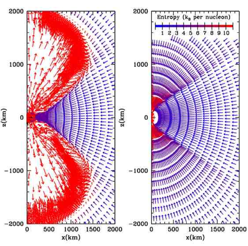
Figure 3: Particle position from our 2-dimensional smooth particle hydrodynamics calculations shaded by entropy. The direction and length of the vectors denote velocity magnitude and direction. The left panel shwos the results at 0.15 s from our standard neutron star “NS2” model. The shocked, high-entropy, material rises and drives an outflow. The right panel shows the absorbing boundary “BH2” model at the same time. Note that the angular momentum alters the flow, but does not slow the material in the equator enough to produce enough viscous heating to drive outflows.

Before we discuss the neutrino fluxes from this suite of calculations, let’s compare the dynamics in the accretion. We expect material to shock as it hits the proto-neutron star, and some of this shocked material will begin to rise, driving convection. These simulations are 2-dimensional. Even without angular momentum, perturbations along our symmetry axis would allow the instability to develop stronger along this axis. But we have studied this in some detail in core-collapse calculations and have minimized this effect (see, for example, Fryer & Heger 2000). However, the fact that the angular momentum axis also lies along the symmetry axis drives convection along our axis of symmetry. The growth of convective instabilities is stabilized by angular momentum gradients and the deceleration of material (along with the fact that our initial condition has an angular momentum gradient which is strongest along the equator), the convection initially grows strongest in the poles. Figure 3 shows the results of our standard calculation showing this outflow. This figure shows the evolution at 0.15 s. The right panel shows the evolution of the corresponding “black hole” simulation with the absorptive boundary. The true innermost stable circular orbit for a slowly rotatign 3 M_⊙ black hole is closer to 20 km, so our 100 km absorption radius understimates the activity from a real black hole. However, we can see that although the angular momentum alters the inflow, it is insufficient to stop it, and the material continues to accrete directly onto the black hole.

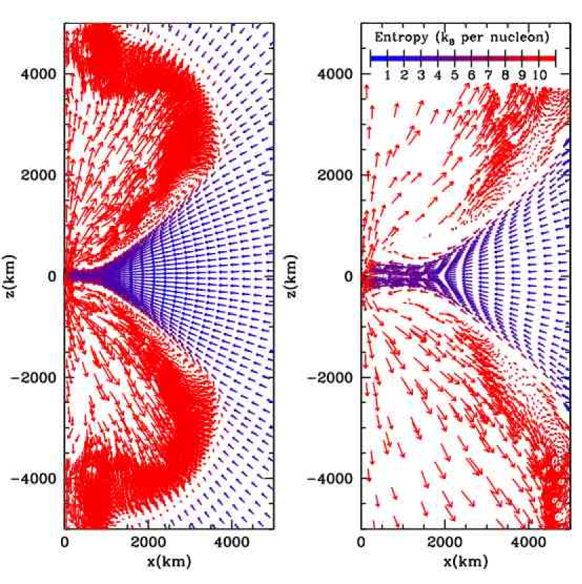
Figure 4: Same as Fig. 3 but for the standard NS2 model 0.3 and 0.45 s from the start of the simulation. Note that the axis has been extended to show the extent of the outflow.

As our neutron star model evolves the outflow expands, constraining the accretion to a funnel roughly $45^{\circ}$ from the plane. Figure 4 shows the evolution of our standard model to 0.3 and 0.45 s. Over half of the inflowing material is ultimately ejected. Not only does the ejected material not contribute to the energy available for neutrino emission, some of the energy of that accreted material goes toward accelerating this ejecta.

Such outflows have been studied for over a decade in supermassive black hole systems such as active galactic nuclei (see Blandford & Begelman 1999) for a review. The amount of potential energy released in the accretion of material onto a compact object is enormous. If this energy is tapped (either by viscous forces or neutrino emission), it can drive an explosion. Rockefeller et al. (2007) and Fryer et al. (2006) have recently applied this physics to stellar-massed compact objects to better understand their simulations of accreting systems. In rotating black hole systems, material hangs up in a disk. Viscous forces that transport out angular momentum also transport energy, driving outflows. What prevents this ejection is cooling (either via photon radiation in the case of supermassive black holes or neutrinos in the case of most collapsing systems). Of course, for black hole systems that do not have a hard surface preventing the inflow of material, high angular momentum is required to prevent the energy from all flowing directly into the black hole. In neutron star systems, outflows (or at least vigorous convection) have been expected for more than a decade (Chevalier 1989; Fryer et al. 1996).

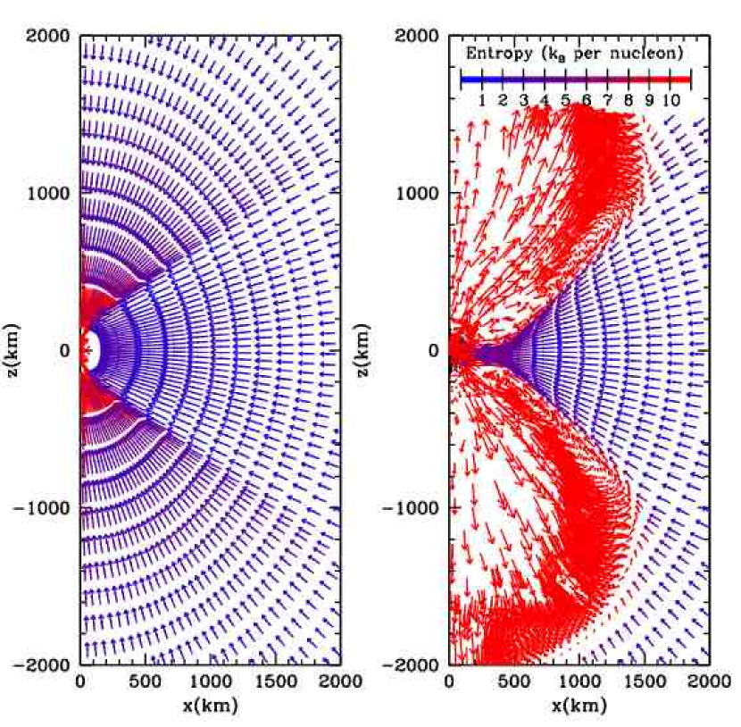
Figure 5: Same as Fig. 3 but for the two faster-rotating models: BH2-Rot10 (left panel) and NS2-Rot2 (right panel). A factor of 10 increase in the square of the specific angular momentum ($j^{2}$) is insufficient to form a disk in our models and the dynamics is not changed significantly.

If the angular momentum were high enough, the infalling material would hang up in a disk. This is most important in the black hole systems. We ran a series of models increasing the specific angular momentum ($j$) a factor of 3 and, for our black hole models, a factor of 10. MacFadyen & Woosley (1999) found that the specific angular momentum must be at least $\sim 10^{17}{\rm cm^{2}s^{-1}}$ (a factor of 1000 higher than our standard $j^{2}$ value). As we can see from Figure 5, our factor of 10 increase in $j$ is not enough to change the fate of material falling back on our “black hole” simulation with its large absorptive boundary. In a true black hole system, the angular momentum available would increase as we move beyond 3 M_⊙ (well above the angular momenta shown in Fig. 2). This is one reason why the collapsar GRB model argues for systems where the black hole mass exceeds 3 M_⊙ when the angular momentum in the star is sufficient to produce an accretion disk. Neutrinos from these systems have been considered in detail elsewhere (MacFadyen & Woosley 1999, Hungerford et al. 2006, Rockefeller et al. 2007) and we do not study them in this paper.

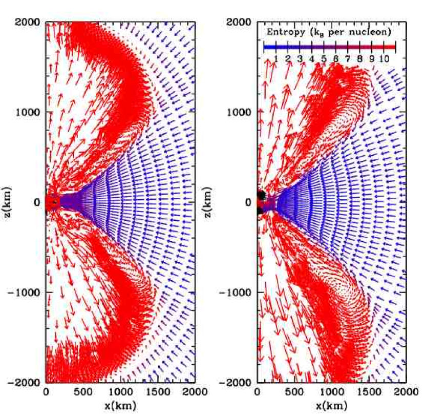
Figure 6: Same as Fig. 3 but for two of our models using hot neutron stars: NS2-Hot1, NS2-Hot2. The dynamics of these simulations is very similar to our cold neutron star runs, but the explosions are slightly stronger.

If the neutron star is still hot and emitting neutrinos, it can also alter the inflow of fallback. Figure 6 shows two simulations with varying amounts of neutrino energy (18 and 36$\times 10^{51}{\rm ergs\,s^{-1}}$) arising off the neutron star surface. The effect on the dynamics is minimal, although a slight increase in the velocity (and hence position at a given time) can be seen. As we shall see below, the neutrinos emanating from the proto-neutron star surface will dominate the total neutrino flux in such cases. But we don’t expect these high luminosities at 10 s and the accretion luminosity will dominate at these later times. But at early times, the modification of the downflow on the neutrino opacities is the dominant effect.

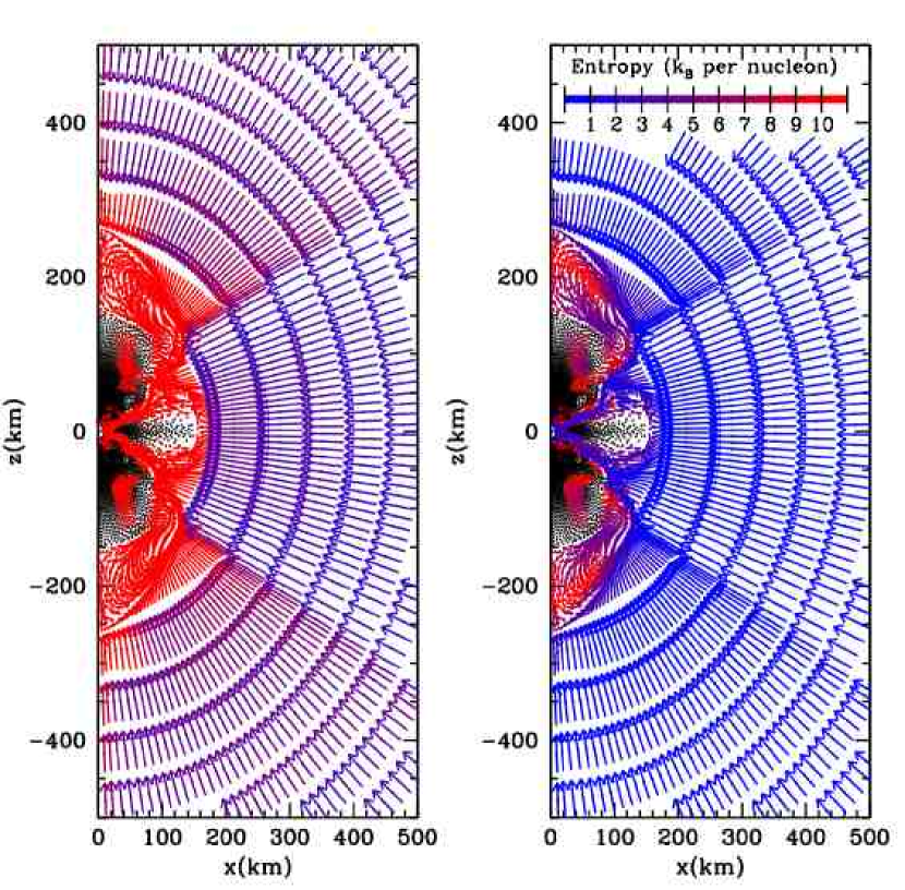
Figure 7: Same as Fig. 3 but for a neutron star models with accretion rates of 0.001 and 0.1 M_⊙ s^-1.

Finally, we have varied the infall rate from 0.001 to 0.1 M_⊙ s^-1. The effect this has on the dynamics is shown in Figure 7. As with many of our models, the nature of the dynamics is not altered significantly by these changes. But we shall see that the neutrino flux very much depends on the accretion rate.

3.3 Neutrino Emission

We found in the last section that the dynamical behavior of the fallback was relatively insensitive to both uncertainties in the numerics as well as uncertainties initial conditions: e.g. fallback rate and rotation. But what about the neutrino luminosity? First let’s study the uncertainties in the numerics. Fig 8 shows the neutrino luminosity and mean energy for 3 different models studying the numerical effects (both the artificial viscosity and the treatment of the inner boundary) on the calculation. The variations in the viscosity and the inner boundary lead to differences that are less than a factor of 2 in the neutrino luminosity and 5% variations in the neutrino mean energy. Many of these errors could be dominated by the explicit transport scheme used in these calculations and it is possible that these errors can be significantly diminished with implicit schemes that are more stable.

Figure 8 also shows the results for a fast rotating NS model (NS-Rot2). With the low angular momenta in our calculations based on the rotation velocities in the inner core material of massive stars (Fig. 2), rotation does not alter the neutrino luminosity noticeably. Black hole systems depend more sensitively on the rotation because it is the angular momentum that prevents the material from accreting directly into our black hole. But as we expected from the fact that our angular momentum is too low to produce accretion disks, the neutrino emission from our black hole systems is negligible (Fig. 9). In such low-angular momentum systems, we expect essentially no emission after the collapse of the neutron star down to a black hole. Contrast this to typical collapsar conditions, where the material falling back onto the black hole has enough angular momentum to hang up in a disk and its falback accretion rate is high enough to produce high-density, high-temperature structures. In this case, the neutrino emission from a black hole can be quite large - with luminosities on par with the neutrino burst of the original collapse (MacFadyen & Woosley 1999; Hungerford et al. 2006; Rockefeller et al. 2007).

In our models, the $\mu$ and $\tau$ neutrinos tend to be an order of magnitude lower than the corresponding electron neutrino fluxes. So our assumption that most of the neutrinos are emitted as electron or anti-electron neutrinos is reasonably valid. Hungerford et al. (2006) and Rockefeller et al. (2007) found that for collapsar models, the $\mu$ and $\tau$ neutrinos make up a sizable fraction of the total emission. At higher accretion rates (and higher angular momentum in the infalling material), the fraction of the luminosity emitted in $\mu$ and $\tau$ neutrinos will likely increase.

The strongest dependency on our initial conditions in the mass accretion rate. Figure 10 shows the neutrino emission from 3 different accretion rates onto our neutron star surface. Our basic potential energy released estimate would argue that the neutrino luminosity scales with the accretion rate. And this trend is basically true for our simulations. However, note that the electron and anti-electron neutrinos for our highest accretion rate (0.1 M_⊙ s^-1) case are not quite an order of magnitude higher than our standard accretion rate (0.01 M_⊙ s^-1). This is because the electron neutrinos become trapped in this highest accretion rate case, lowering the escaping luminosity. The $\mu$ and $\tau$ remain nearly an order of magnitude higher as they are not trapped in any of our simulations.

Figure 11 shows the neutrino emission for 3 different “hot” neutron star models. Fallback contributes an additional 10-20% of the luminosity on average for the NS2-hot2 model, 20-40% to the NS2-hot1 model, and over 50% to the NS1-hot model. The neutrino energy is also altered by an amount comparable to the change in the luminosity. Although a hot neutron star may dominate the neutrino luminosity, fallback clearly can contribute a sizable fraction of the observed neutrino flux.

Finally, note that in general, our predicted fallback neutrino energies are high. The most notable exception is that the mean neutrino energy is 5-10 MeV cooler for our low accretion-rate simulations. As the accretion rate decreases, so too will the mean energy of the emitted neutrinos.

4 Conclusions

Fallback (of at least 0.1 M_⊙) is likely to occur in normal ($10^{51}$ erg) supernova explosions from stars with initial masses of 12 M_⊙ or greater. With energy-injected (more realistic than piston-driven) explosion calculations, this fallback occurs quickly, generally in the first 15 s and peak accretion rates in the 0.01-0.1 M_⊙ s^-1 range should be expected. If the engine stays active long after the launch of the supernova shock, the total fallback will be lower. But neutrino engines weaken significantly quickly after the shock is launched and the material above the neutrinosphere (absorbing the energy) is ejected. Magnetic-driven explosions could be very different. The mechanism for this fallback is essentially that proposed by Colgate (1971) whereby the outflowing material decelerates as it pushes against the material above it, ultimately decreasing its velocity below the escape velocity and causing it to fall back onto the proto-neutron star. This means that the bulk of the fallback is fairly insensitive to the structure on the outer envelope of the star (so fallback is roughly the same whether or not the star is in a binary).

Our multi-dimensional simulations of this fallback suggest that not all of this fallback material is actually incorporated into the proto-neutron star. Some of it flows out of the system. The corresponding neutrino luminosity is also lower, both because less material is accreted and some of the energy released goes toward driving outflows. But the neutrinos from fallback could still dominate the neutrino emission from a proto-neutron star 10 s into the explosion.

At this time, observations of neutrinos from supernovae are limited to those of supernova 1987A (Hirata et al. 1987, Bionta et al. 1987). With only 20 neutrinos over $\sim$15 s, it is difficult to place many constraints on the fallback. Some authors have claimed that claimed that the late-time neutrinos could not be easily explained by a cooling neutron star (e.g. Suzuki & Sato 1987), but others have argued that the observed neutrino signal is consistent with neutrinos diffusing out of a hot proto-neutron star (Burrows & Lattimer 1987; Bruenn 1987) . In our neutron-star forming models, fallback ends within the first 10-15 s, comparable to the duration of the observed neutrino burst and the flux is consistent with our more standard accretion rates. The observations are consistent with fallback, but could easily be explained by a neutron star without any fallback. Given that the progenitor star is believed to be greater than 15 M_⊙, fallback is likely to have occured. But with the current errors in the time-dependent luminosity, it is difficult to determine whether or not accretion is taking place.

If we assume fallback accretion did occur, the fact that the mean neutrino energy appears to be dropping with time in the observations suggests that the accretion rate is dropping at 10 s. But neutrinos are still observed at 10 s. Unless the fallback material has considerable angular momentum, the compact remnant is not a black hole at 10 s. In addition, because the accretion rate is dropping dramatically at this time, it is unlikely that the remnant will accrete much additional mass. It will remain a neutron star. In our fallback calculations, systems that accrete enough material to form a black hole are either already a black hole at 10 s or still accreting rapidly at 10 s, neither of which is supported by the observations. But we really need a better neutrino signal to say anything definitive.

With such high accretion rates, fallback can easily dominate the neutrino luminosity after a few seconds, more than doubling the emission from the neutron star at thearly times. If we wish to study neutrino opacities in the supernova explosion, we will have to be able to calculate this fallback. It may be possible to estimate the fallback rate from detailed study of supernova light-curves. Fortunately, any system that is detected in neutrinos will have a wealth of data in photons of all wavelengths.

If the fallback rate is high, the infalling material will alter the position of the neutrinosphere, and the problem becomes nearly as complex as the supernova explosion modeling itself. We have only touched the surface on the difficulties in modeling such systems. In this paper, we have not addressed the production or feedback of magnetic fields, which may definitely alter the fate of the fallback. We have also not discussed the nuclear yields from the ejecta (a first paper on this is by Fryer et al. 2007 and we plan future projects studying this nucleosynthesis). However, note that the old “wind” r-process picture will not work in any system with fallback (stars more massive than $\sim 12$M_⊙). The matter trajectories just can’t be explained by the wind solution in the cases where fallback dominates the motion near the neutron star. We also have not studied the actual accretion onto the neutron star in detail. Note that the final neutron star masses in Table 1 assumed no mass ejecta. But as we have found in this study, over half of the fallback material may be ejected, leading to smaller neutron star masses and a narrower mass range for these neutron stars.

Table 1: Fallback Results

Progenitor	Explosion	Fallback	Neutron Star	Peak Accretion	Energy
Mass (M⊙)	Energy (1051 erg)	Mass (M⊙)	Mass (M⊙)	Rate (M${}_{\odot}{\rm s^{-1}}$)	Released (1051 erg)
12
	0.55	0.33	1.64	$>$0.02	120
	0.92	0.23	1.54	$>$0.01	86
	2.4	0.030	1.34	$>$0.003	11
	3.6	0.015	1.33	$>$0.001	5.6
15
	0.9	0.34	1.75	$>$0.05	130
	1.65	0.25	1.66	$>$0.05	93
	7.0	0.11	1.52	$>$0.02	41
	17	0.08	1.49	$>$0.01	30
23
	1.25	2.2	3.9	$>$0.15	820
	2.0	1.75	3.45	$>$0.1	650
	2.5	0.86	2.56	$>$0.1	320
	6.6	0.02	1.72	$>$0.01	7.5

Table 2: 2-D Simulations

Model	Accretion	Boundary	Angular	Neutron Star	Other
Name	Rate (M⊙ s-1)	Condition	Momentum	Luminosity ($10^{51}{\rm ergs^{-1}}$)
NS3	$10^{-3}$	$\rho>10^{10},Y_{e}<0.3$	$3\times 10^{15}{\rm cm^{2}s^{-1}}$	0.
BH3	$10^{-3}$	$r<100$ km	$3\times 10^{15}{\rm cm^{2}s^{-1}}$	0.
NS2	$10^{-2}$	$\rho>10^{10},Y_{e}<0.3$	$3\times 10^{15}{\rm cm^{2}s^{-1}}$	0.
NS2-Rot2	$10^{-2}$	$\rho>10^{10},Y_{e}<0.3$	$10^{16}{\rm cm^{2}s^{-1}}$	0.
NS2-Hot1	$10^{-2}$	$\rho>10^{10},Y_{e}<0.3$	$3\times 10^{15}{\rm cm^{2}s^{-1}}$	18.
NS2-Hot2	$10^{-2}$	$\rho>10^{10},Y_{e}<0.3$	$3\times 10^{15}{\rm cm^{2}s^{-1}}$	36.
NS2alpha	$10^{-2}$	$\rho>10^{10},Y_{e}<0.3$	$3\times 10^{15}{\rm cm^{2}s^{-1}}$	0.	$2\times\alpha$
NS2bound	$10^{-2}$	$\rho>10^{11},Y_{e}<0.1$	$3\times 10^{15}{\rm cm^{2}s^{-1}}$	0.	$2\times\alpha$
BH2	$10^{-2}$	$r<100\,km$	$3\times 10^{15}{\rm cm^{2}s^{-1}}$	0.
BH2-Rot0	$10^{-2}$	$r<100\,km$	0.	0.
BH2-Rot2	$10^{-2}$	$r<100\,km$	$10^{16}{\rm cm^{2}s^{-1}}$	0.
BH2-Rot10	$10^{-2}$	$r<100\,km$	$3\times 10^{16}{\rm cm^{2}s^{-1}}$	0.
NS1	$10^{-1}$	$\rho>10^{10},Y_{e}<0.3$	$3\times 10^{15}{\rm cm^{2}s^{-1}}$	0.
NS1hot	$10^{-1}$	$\rho>10^{10},Y_{e}<0.3$	$3\times 10^{15}{\rm cm^{2}s^{-1}}$	36.
BH1	$10^{-1}$	$r<100\,km$	$3\times 10^{15}{\rm cm^{2}s^{-1}}$	0.

Figure 1: Fallback mass as a function of time from the launch of the explosion for 3 different progenitor masses (one progenitor for each panel) and a range of explosion energies (1 foe = $10^{51}{\rm erg}$). Most of the fallback is finished after 15 s. Note that for a given explosion energy, the more massive the progenitor, the more fallback that occurs. But also note that for a standard “1 foe” explosion, our 12 M_⊙ model still accretes 0.2 M_⊙ in roughly 10 s corresponding to an accretion rate of 0.02 M${}_{\odot}{\rm s^{-1}}$.

Figure 2: Angular momentum versus enclosed mass for 6 different stellar models: standard 20 M_⊙ model (solid), standard 12 M_⊙ model (dotted), standard 35 M_⊙ model (dashed), 20 M_⊙, $N^{2}_{\mu}=0.1$ model (short-dot dashed), 20 M_⊙ $B_{\mu},B_{\phi}=0.1$ model (long-dot dashed), and a 100 km s^-1 model with no magnetic braking. The first 5 models are from Heger et al. (2005), the last model is from Heger et al. (2000). The angular momenta used in our simulations is shown by the circle (standard) and square dots.

Figure 8: Neutrino Luminosity (left panel) and energy (right panel) versus time for electron, anti-electron and $\mu,\tau$ neutrinos as a function of time for 3 different models: NS2-Rot2, our fast rotating NS model (solid line), NS2bound, the simulation with more restrictive accretion criteria (dotted line), and NS2alpha, the simulation with the enhanced values for viscosity (dashed line). Not that all models agree to within a factor of 2 in the lumosity and 5% in neutrino energy at all times.

Figure 9: Neutrino Luminosity (left panel) and energy (right panel) versus time for electron, anti-electron and $\mu,\tau$ neutrinos as a function of time for 3 different black hole models: BH2 (solid), BH2-Rot0 (dotted),. BH2-Rot10 (dashed). These results confirm that the accreting material with such low angular momenta falls directly onto the black hole without any appreciable neutrino emission.

Figure 10: Neutrino Luminosity (left panel) and energy (right panel) versus time for electron, anti-electron and $\mu,\tau$ neutrinos as a function of time for 3 different accretion rates: 0.001-NS3 (dashed), NS2 0.01 (solid), and NS1 0.1 (dashed)  M_⊙ s^-1. Here the results depend nearly linearly on the accretion rate and for the highest accretion rates, the neutrino luminosity is roughly $10^{52}$ ergs s^-1.

Figure 11: Neutrino Luminosity (left panel) and energy (right panel) versus time for electron, anti-electron and $\mu,\tau$ neutrinos as a function of time for 3 different neutron star models with emitting neutron stars: NS2-hot1 (dotted), NS2-hot2 (solid), NS1-hot (dashed). Fallback contributes an additional 10-20% of the luminosity on average for the NS2-hot2 model, 20-40% to the NS2-hot1 model, and over 50% to the NS1-hot model. The neutrino energy is also altered by an amount comparable to the change in the luminosity. Although a hot neutron star may dominate the neutrino luminosity, fallback clearly can contribute a sizable fraction of the observed neutrino flux.

References

- Arnett (1971) Arnett, W.D. 1971, ApJ, 163, 11
- Bionta et al. (1987) Bionta, R.M. et al. 1987, PRL, 58, 1494
- Blandford & Begelman (1999) Blandford, R.D. & Begelman, M.C. 1999, MNRAS, 303, L1
- Bruenn (1987) Bruenn, S.W. 1987, PRL, 59, 938
- Burrows & Lattimer (1987) Burrows, A., & Lattimer, J.M. 1987, ApJ, 318, L63
- Bisnovatyi-Kogan & Lamzin (1984) Bisnovatyi-Kogan, G.S., & Lamzin, S.A. 1984, Soviet Astron., 28, 187
- Chevalier (1989) hevalier, R.A. 1989, ApJ, 346, 847
- Colgate (1971) Colgate, S.A. 1971, ApJ, 163, 221
- Frölich et al. (2006) Frölich, C. et al. 2006, ApJ, 637, 415
- Fryer et al. (1996) Fryer, C.L., Benz, W., & Herant, M. 1996, ApJ, 460, 801
- Fryer et al. (1999) Fryer, C.L., Colgate, S.A., & Pinto, P.A. 1999, ApJ, 511, 885
- Fryer & Heger (2000) Fryer, C.L., & Heger, A. ApJ, 541, 1033
- Fryer & Kalogera (2001) Fryer,. C.L., & Kalogera, V. 2001, ApJ, 554, 548
- Fryer (2003) Fryer, C.L. 2003, IJMPD, 12, 1795
- Fryer et al. (2006) Fryer, C.L., Herwig, F., Hungerford, A., Timmes, F.X. 2006, ApJ, 646, L131
- Fryer & Young (2007) Fryer, C.L., & Young, P.A. 2007, ApJ, 659, 1438
- Heger et al. (2000) Heger, A., Langer, N., & Woosley, S.E. 2000, ApJ, 528, 368
- Heger et al. (2000) Heger, A., Woosley, S.E. & Spruit, H.C., 2005, ApJ, 626, 350
- Herant et al. (1994) Herant, M., Benz, W., Hix, W.R., Fryer, C.L., & Colgate, S.A. 1994, ApJ, 435, 339
- Hirata et al. (1987) Hirata, K. et al. 1987, PRL, 58, 1490
- Hungerford et al. (2006) Hungerford, A.L., Rockefeller, G., & Fryer, C.L. 2006, Il Nuovo Cimento, 121, 1327
- Keil et al. (1996) Keil, W., Janka, H.-Th., Müller, E. 1996, ApJ, 473, L111
- MacFadyen et al. (1999) MacFadyen, A.I., & Woosley, S.E. 1999, ApJ, 524, 262
- MacFadyen et al. (2001) MacFadyen, A.I., Woosley, S.E., & Heger, A. 2001, ApJ, 550, 410
- Reddy et al. (1999) Reddy, S., Prakash, M., Lattimer, J.M., & Pons, J.A. 1999, Phys. Rev. C, 59, 2888
- Rockefeller et al. (2007) Rockefeller, G., Fryer, C.L., & Li, H. submitted to ApJ, astro-ph/0608028
- (27) Suzuki, H., & Sato, K. 1987, PASJ, 39, 521
- Woosley (1989) Woosley, S.E., 1989, NY Acad. Sci. Ann., 571, 397
- Young et al. (2006) Young, P.A., Fryer, C.L., Hungerford, A., Arnett, D., Rockefeller, G., Timmes, F.X., Voit, B., Meakin, C., & Eriksen, K.A. 2006, ApJ, 640, 891
- Young & Fryer (2007) Young, P.A., & Fryer, C.L. 2007, ApJ, 664, 1033
- Young et al. (2008) Young, P.A. et al. 2008, in preparation