Torque magnetometry study of metamagnetic transitions in single-crystal HoNi₂B₂C at $\textbf{{T}}\approx$ 1.9 K

Abstract

Metamagnetic transitions in single-crystal rare-earth nickel borocarbide HoNi₂B₂C have been studied at $T\approx$ 1.9 K with a Quantum Design torque magnetometer. This compound is highly anisotropic with a variety of metamagnetic states at low temperature which includes antiferromagnetic, ferrimagnetic, non-collinear and ferromagnetic-like (saturated paramagnet) states. The critical fields of the transitions depend crucially on the angle $\theta$ between applied field and the easy axis [110]. Measurements of torque along the $c$-axis have been made while changing the angular direction of the magnetic field (parallel to basal tetragonal $ab$-planes) and with changing field at fixed angle over a wide angular range. Two new phase boundaries in the region of the non-collinear phase have been observed, and the direction of the magnetization in this phase has been precisely determined. At low field the antiferromagnetic phase is observed to be multidomain. In the angular range very close to the hard axis [100] ($-6^{\circ}\lesssim\phi\lesssim 6^{\circ}$, where $\phi$ is the angle between field and the hard axis) the magnetic behavior is found to be “frustrated” with a mixture of phases with different directions of the magnetization.

I Introduction

The rare-earth nickel borocarbides (RNi₂B₂C where R is a rare-earth element) have attracted considerable interest in the last decade because of their unique superconducting and/or magnetic properties (see reviews don1 ; muller ; thal ; gupta ). The crystal structure of RNi₂B₂C is a body-centered tetragonal with space group $I4/mmm$ muller ; thal ; gupta ; sieg ; lynn , a layered structure in which Ni₂B₂ layers are separated by R-C planes stacked along the $c$-axis. The R ions are situated at the corners and in the center of the crystal unit cell. Conducting (and superconducting) properties are determined mainly by Ni $3d$ electrons, while magnetic properties are dictated by localized electrons in the R $4f$-shell. Long-range magnetic order is thought to result from the indirect RKKY interaction, mediated through conducting electrons. This gives rise to different types of antiferromagnetic (AFM) order of the $4f$-ions at low temperatures muller ; thal ; gupta ; lynn . Borocarbides with R = Tm, Er, Ho, Dy show coexistence of superconductivity and long-range magnetic order.

Although the borocarbides were studied quite intensively, certain important issues remain open. We report a torque magnetometry study of metamagnetic transitions at low temperature ($T\approx 1.9$ K) in a single-crystal magnetic superconductor HoNi₂B₂C. Torque magnetometry is sensitive only to the component of the magnetization normal to both the applied field and the torque and is thus useful in the study of magnetic anisotropy. The choice of the subject was determined by its interesting magnetic properties, which cannot be considered as fully understood to date, and by the circumstance, that torque magnetometry was applied to the borocarbides so far only in limited cases winzer2 ; canf . The magnetic properties of HoNi₂B₂C, a superconductor with critical temperature T${}_{c}\approx 8.7$ K, are characterized by (i) large anisotropy and (ii) availability of different field-induced magnetic phases at low temperatures don1 ; muller ; thal ; gupta ; lynn ; daya ; canf ; kalats ; amici ; salamon . Three magnetic transitions occur in a narrow temperature interval, when moving from the paramagnetic state in low field below $T_{c}\approx 8.7$ K. The first two transitions (at 6.0 K and 5.5 K) result in two incommensurate AFM phases, described in detail in muller ; thal ; lynn . Below $T_{N}\approx 5.2$ K, the transition to a commensurate AFM phase occurs. This AFM phase is a $c$-axis modulated magnetic structure consisting of Ho-moments ferromagnetically aligned in the tetragonal basal $(ab)$ planes along the [110] axis and stacked antiferromagnetically in the $c$-direction. The easy magnetic axis [110] was found experimentally and supported by theory thal ; lynn ; canf ; kalats ; amici . In a tetragonal lattice four equivalent easy directions $\langle 110\rangle$ are expected. The four $\langle 100\rangle$ axes are hard directions. No appreciable magnetization was found in the direction perpendicular to the $ab$-planes (along the $c$-axis) in fields up to 6 T canf , so it is commonly assumed that the Ho magnetic moments always lie in the $ab$-planes roughly parallel to one of the $\langle 110\rangle$ axes.

In the temperature range below $T\approx$ 4 K, several metamagnetic transitions (of first order) were found, depending on the magnitude of the magnetic field applied parallel to the $ab$-planes and the angle $\theta$ between the field and the nearest easy axis $\langle 110\rangle$. Below a critical field $H_{m1}$, the commensurate AFM phase, characterized by alternating ferromagnetically ordered $ab$-planes with the Ho moments in neighboring planes in opposite directions, is stable. This phase can be symbolized by ($\uparrow\downarrow$) canf ; kalats ; amici , which means that the Ho moments are parallel to one of the easy directions (say, [110]) in one half of the $ab$ planes and parallel to the opposite direction (that is, to 1̄1̄0) in the other half.

With increasing field, at $H=H_{m1}$ a transition to a collinear ferrimagnetic phase takes place. This phase can be symbolized as ($\uparrow\uparrow\downarrow$). Spins in two thirds of the $ab$-planes are parallel to one easy axis, while those in the remaining one third are antiparallel. It yields one third of the maximum possible magnetization that the Ho ions can provide. The next metamagnetic transition at higher field $H=H_{m2}>H_{m1}$ results in the non-collinear phase ($\uparrow\uparrow\rightarrow$) canf . It was assumed in the existing theories kalats ; amici in this case that two thirds of the spins are parallel to one of the easy axes (as in the preceding ferrimagnetic phase), but the remaining one third is perpendicular to that axis. In this model the net magnetization is thus predicted to make an angle $\Phi=26.6^{\circ}$ with the easy axis. The nature of this non-collinear phase turns out to be, however, not so simple muller ; thal ; camp ; detlef ; schneider . In particular, the models kalats ; amici assume a magnetic structure modulated along the $c$-axis ($q=2/3$ $c^{*}$); whereas, neutron diffraction studies show that this phase is modulated along the $a(b)$-axis ($q\approx 0.58$ $a^{*}$) camp ; detlef ; schneider . Finally, at the field $H_{m3}$, a transition to the ($\uparrow\uparrow$) phase, the saturated paramagnetic state in which the spins are aligned ferromagnetically parallel to the $\langle 110\rangle$ axis nearest to the direction of the applied field, occurs. According to Ref. canf , if the field is directed along or rather close to a $\langle 110\rangle$ axis, within the angular region $-6^{\circ}\lesssim\theta\lesssim 6^{\circ}$, the ($\uparrow\downarrow$)–($\uparrow\uparrow\downarrow$)–($\uparrow\uparrow$) sequence of transitions takes place. For larger $\theta$ (outside this range, greater than $6^{\circ}$ and less than $45^{\circ}$ from the same $\langle 110\rangle$ axis) the whole sequence of possible transitions [($\uparrow\downarrow$)–($\uparrow\uparrow\downarrow$)–($\uparrow\uparrow\rightarrow$)–($\uparrow\uparrow$)] would be observed. The suggested $H$-$\theta$ diagram of metamagnetic transitions in HoNi₂B₂C at $T=2$ K based on longitudinal magnetization measurements canf is shown by the solid lines in Fig. 1.

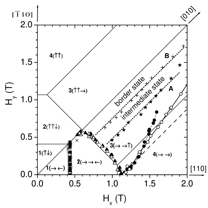
Figure 1: The phase diagram for metamagnetic transitions in single crystal HoNi₂B₂C at low temperature. Symbols of different magnetic states are defined in the main text of the paper. The phase-boundary lines (in the angular range between an easy $\langle 110\rangle$ and a hard $\langle 010\rangle$ axis) indicated by the filled and empty squares, triangles and circles represent results of measurements at $T\approx 1.9$ K (LM and HM torque chips, respectively) from this study. The lines A and B, formed by stars and crosses, are new boundaries of metamagnetic states revealed in this study. Solid lines represent boundaries reported canf from longitudinal magnetization measurements at $T\approx 2$ K. The dashed line represents the fit for data of this study to Eq. (3) with $H_{m3}=0.79$ T at small $\theta$. The data points $\times$ is indicative of the extent of frustration in the ($\rightarrow\rightarrow\leftarrow$) ferrimagnetic state.

Since magnetic anisotropy tends to align the Ho magnetic moments along the $\langle 110\rangle$ axis, it is clear that angular dependence of the critical fields ($H_{m1}$, $H_{m2}$, and $H_{m3}$) must be periodic with a period of $90^{\circ}$ if the four easy axes are equivalent. The angular dependences of the critical fields in the $ab$-plane were previously studied mainly with a standard magnetometer canf which measures the magnetization along the applied field (the longitudinal magnetization). For those studies, the magnetic field was rotated away from an easy axis [110] in the plane perpendicular to the $c$-axis. Measurements were taken mainly in the range $-45^{\circ}\lesssim\theta\lesssim 45^{\circ}$. The results for the collinear phases [($\uparrow\downarrow$), ($\uparrow\uparrow\downarrow$), ($\uparrow\uparrow$)] were reasonably well explained by theoretical models kalats ; amici which considered the interactions between moments in an $ab$-plane to be only ferromagnetic. Since neutron scattering camp ; detlef ; schneider shows that the non-collinear phase ($\uparrow\uparrow\rightarrow$) is, however, not modulated in the $c$-direction, that phase should be described by a much more complicated model.

Torque magnetometry has some distinct advantages as compared with longitudinal magnetometry in studies of magnetically anisotropic compounds like HoNi₂B₂C. A magnetometer of this type measures the torque $\vec{\tau}=\vec{M}\times\vec{H}$, so that $\tau=MH\sin(\beta)$, where $\beta$ is the angle between external magnetic field and magnetization. This allows precise determination of the direction of the net magnetization in each phase. When the magnetization in a material does not align with the applied magnetic field vector, the torque on the sample is actually a measure of the magnetic anisotropy energy. The torque is determined by both, magnitude and direction of the magnetization. Thus, changes in magnetization direction (or rotation of the magnetization) at metamagnetic transitions are easily seen with torque magnetometry, but the standard longitudinal magnetometry is much less sensitive, particularly near the hard axis for this borocarbide.

Three specific problems concerning low-temperature magnetic states of HoNi₂B₂C have been targeted in this study. First is the precise determination of the magnetization direction in the non-collinear phase and its dependence on magnitude of the field. The second is connected with the four possible equivalent easy direction $\langle 110\rangle$ axes. Under these conditions, if a sample is cooled in zero field, some kind of frustrated or multidomain (or, at least, two-domain) state can be expected as has been pointed out in studies winzer1 ; winzer2 of the related magnetic borocarbide DyNi₂B₂C. The third question is whether different easy $\langle 110\rangle$ axes are really equivalent in light of the magnetoelastic tetragonal-to-orthorhombic distortions where the unit cell is shortened about 0.19 % along the [110] direction, in which the long-range ordered Ho moments are aligned kreysig as compared to its length in the perpendicular [$\bar{1}10$] direction at low temperature (1.5 K). Analysis of the torque behavior in a wide angular range of magnetic field directions can answer this question.

Results of this study reveal some important new features of the metamagnetic phases in HoNi₂B₂C and transitions between them, including two new phase boundaries. Presentation and discussion of results proceed as follows: 1) the angular phase diagram of metamagnetic transitions reported here are compared with the only previous detailed study canf and with the main theoretical models kalats ; amici ; 2) some new important peculiarities of these states and the transitions between them are discussed.

II Experimental

The PPMS Model 550 Torque Magnetometer (Quantum Design) with piezoresistive cantilever was used in this study. The HoNi₂B₂C single crystal was grown by Canfield ming . The crystal was carefully cut to provide a sample weighing in the range 0.1–0.15 mg in the form of a plate ($0.4\times 0.32\times 0.26$ mm³) with the $c$-axis perpendicular to the plate surface and $a$, $b$ axes parallel to the edges. The sample was mounted on the torque chip in a PPMS rotator so that the torque measured was along the $c$-axis of the crystal. During rotation of the sample the $c$-axis was almost precisely perpendicular to the applied field at all times. This crystal was used previously in our studies of the magnetic phase diagram of HoNi₂B₂C daya . Those measurements were reproduced on several different single crystals from Canfield’s lab. We also made torque measurements at representative fields and angles on another sample cut from a single crystal from a different batch of Canfield’s crystals and obtained similar results. Thus, we expect that the results presented here are fully representative of Canfield’s crystals, which seem to set the standard for work on this family of compounds.

Two types of the PPMS torque chips are used in this study: 1) Low Moment (LM) (two-leg) chip with RMS torque noise level about $1\times 10^{-9}$ Nm and maximum allowable torque about $5\times 10^{-5}$ Nm; and 2) High Moment (HM) (three-leg) chip with RMS torque noise level about $2\times 10^{-8}$ Nm and maximum allowable torque about $1\times 10^{-4}$ Nm. The maximal applied fields for LM and HM chips were limited to 2 T and 3.5 T, respectively, to reduce breakage.

It is known wille (but usually not taken into account) that at large torque the orientation change of the sample due to twisting of the cantilever itself is no longer negligible. This can cause an error in angular position of the high-field metamagnetic transitions. The angular coefficient factor for a silicon piezoresistive cantilever of microscopic size (about 0.2 mm in width) can be about $(0.3-0.5)^{\circ}/\mu$Nm wille . For the HM chip of the PPMS device this coefficient is about $0.3^{\circ}/\mu$Nm quantum . Thus, for higher torque ($\tau>1\times 10^{-5}$ Nm) the angular error for critical fields due to twisting of the cantilever can be several degrees. It is also evident that twisting of the cantilever can induce apparent angular asymmetry of metamagnetic transitions for high magnitudes of field and torque. We have observed this effect for the critical field $H_{m3}$, but this asymmetry appears to be rather small (about $1^{\circ}$) even for the highest fields and torques in this study.

In addition to the error due to twisting of the cantilever, another important contribution to total error is non-linearity, when the torque is rather close to the maximum allowable value. This can cause underestimation of the measured torque (and magnetization) and, thus, the magnitude of the critical field $H_{m3}(\theta)$. This particular error should be higher for the LM chip in comparison to the HM chip. In this study both the LM and HM chips gave practically the same numerical results for the torque and angular dependence of the metamagnetic transitions below 1.5 T (this field region includes the first two metamagnetic transitions for any angular position of the field, and the third transition to a saturated paramagnetic ($\uparrow\uparrow$) phase for angular positions not too far from the easy axis). For the higher field range (1.5–2.0 T), however, the HM chip gave systematically higher values of the measured torque than the LM chip. The difference increases with field, so that at $H=2.0$ T the ratio of the torque values measured by the HM and LM chips is about 1.5. It is clear that above 1.5 T (where the torque was close to or even larger than $1\times 10^{-5}$ Nm) the HM chip measures more precisely than the LM one.

In general, we believe that the results of this study obtained below 1.5 T can be considered as reliable with accuracy for the angle values for magnetic transitions being about $\pm 1^{\circ}$. For higher field, $H\gtrsim 2$ T, where the torque of the sample was close to maximum allowable values, the precision is far less. For precise measurements in higher fields, a sample with smaller mass (and dimensions) should be used, but we were not able to prepare and orient a significantly smaller sample. Although the sample studied was mounted carefully with the $c$-axis perpendicular to the applied field, some misalignment cannot be excluded. It is estimated that this tilting is no more than $5^{\circ}$, which would produce less than a 1 % error in the measured magnitudes of the critical fields of the metamagnetic transitions. For samples with smaller dimensions this error can be far larger. We have estimated demagnetization fields to be no more than 30-40 mT at the highest fields which would affect the accuracy of angular measurements of at most $1-2^{\circ}$. Torque measurements were made by changing the magnetic field for different constant angles and by sweeping the angle for different fixed values of magnetic field at one temperature $T\approx$ 1.9 K only.

III Results and discussion

During discussion of the results obtained, the angular position of the applied magnetic field will be described by different but related angles shown in Fig. 2. The first is the angle, $\theta_{r}$, the rotator position of the torque magnetometer. The second is the angle $\theta$ between the applied field and the nearest easy axis $\langle 110\rangle$. In some cases it is more convenient to use the angle $\phi$ between the field and the nearest hard axis $\langle 100\rangle$. Finally, the angle $\beta$ between the external magnetic field and the magnetization (which does not coincide with angle $\theta$ for some metamagnetic phases studied) is also very important for understanding the torque results.

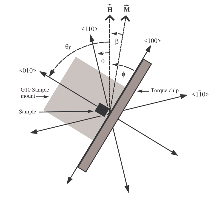
Figure 2: Angles used in the discussion. When mounted on the rotator with $\theta_{r}=0$ the applied field $\vec{H}$ lies along the $\langle 010\rangle$ crystal axis. The sample is rotated $\theta_{r}$ (indicated by the PPMS rotator) with the field remaining fixed. The angle $\theta$ is between the nearest $\langle 110\rangle$ crystal axis (easy axis) and the applied field, and $\phi$ is the angle between the nearest $\langle 100\rangle$ crystal axis (hard axis). The angle between $\vec{M}$ and $\vec{H}$ is $\beta$.

After the sample is mounted in the torque magnetometer, the easy axes $\langle 110\rangle$ (or hard axes $\langle 100\rangle$) in terms of the angular position of the rotator, $\theta_{r}$, are initially known only approximately (within a few degrees). But their location is determined rather precisely from measured angular dependences of the torque, which are found to be periodic to a good approximation with a period of $90^{\circ}$, as expected. The angles $\theta_{r}=45^{\circ}$, $135^{\circ}$ and $225^{\circ}$ correspond within one degree accuracy to the $\langle 110\rangle$ easy axes. Similarly, $\theta_{r}=0^{\circ}$, $90^{\circ}$, and $180^{\circ}$ correspond to $\langle 100\rangle$ hard axes.

III.1 Angular phase diagram

The angular dependences of the critical fields for all metamagnetic transitions found in this study are summarized in Fig. 3 for the whole angular range studied. They represent results obtained from the field dependence of the torque recorded for different angles and angular dependence of the torque recorded for different fields (see examples in Figs. 4 and 5). The transitions manifest themselves as sharp changes or even jumps of the torque at the critical fields or angles. The critical fields ($H_{m1}$, $H_{m2}$, and $H_{m3}$) for a given angle are defined by the inflection point in the corresponding $\tau(H)$ transition curves with increasing applied magnetic field (Fig. 4). Angles of the transitions for different applied fields are defined in a similar way (Fig. 5). The first ($\uparrow\downarrow$)–($\uparrow\uparrow\downarrow$) (AFM–ferrimagnetic) transition manifests itself clearly for all angles, as do other transitions (see Figs. 4 and 5). For angles rather close to the easy $\langle 110\rangle$ or hard $\langle 100\rangle$ axes some of the metamagnetic transitions show specific unusual features outlined further below. The first transition has considerable hysteresis (Fig.4). For the other two transitions, the field hysteresis is small. Some angular hysteresis is also observed when measuring for increasing and decreasing angle (Fig. 5). For the most part, this hysteresis is not large (1–1.5 degree) and is isotropic. We believe that it is mainly due to the backlash in the rotator. For the angular positions of the field near the hard axis we found an increased angular hysteresis (up to $4^{\circ}$). For this reason, critical angles of the metamagnetic transitions recorded for fixed values of the magnetic field were determined for increasing angle. For some angles the transitions at $H_{m2}$, ($\uparrow\uparrow\downarrow$)–($\uparrow\uparrow\rightarrow$), and at $H_{m3}$, ($\uparrow\uparrow\rightarrow$)–($\uparrow\uparrow$), show a change of sign of the torque (Fig. 4), which clearly indicates a change of direction of the net magnetization from one side of the applied field to the other. The phase-boundary lines determined in this study are compared (Fig. 1) with the phase diagram determined from longitudinal magnetization measurements canf .

In order to compare the first two transitions with previous measurements, they are presented in Fig. 6 on an enlarged scale. The first ($\uparrow\downarrow$)–($\uparrow\uparrow\downarrow$) metamagnetic transition is described well by the angular relation

$$H_{m1}(\theta)=H_{m1}(0)/\cos(\theta)$$ (1)

[with $H_{m1}(0)=0.437$ T], shown by the solid curve in Fig. 6 (see also the corresponding straight phase-boundary line in Fig. 1). This is consistent with that found from measurements of the longitudinal magnetization for increasing field canf , except that $H_{m1}(0)\approx 0.41$ T in canf , which was fitted with theoretical models kalats ; amici . A pronounced hysteresis is found for this transition (Fig. 4) with $H_{m1}$ obtained for decreasing field about 0.04 T below that for increasing field. This angular dependence (1) is understood in terms of the Ho moments remaining aligned along the [110] axis when the magnetic field is rotated from it in the $ab$-plane, as long as the angle of rotation does not exceed $45^{\circ}$. Thus, only the projection of the field on the [110] axis is important (see the phase diagram in Fig. 1).

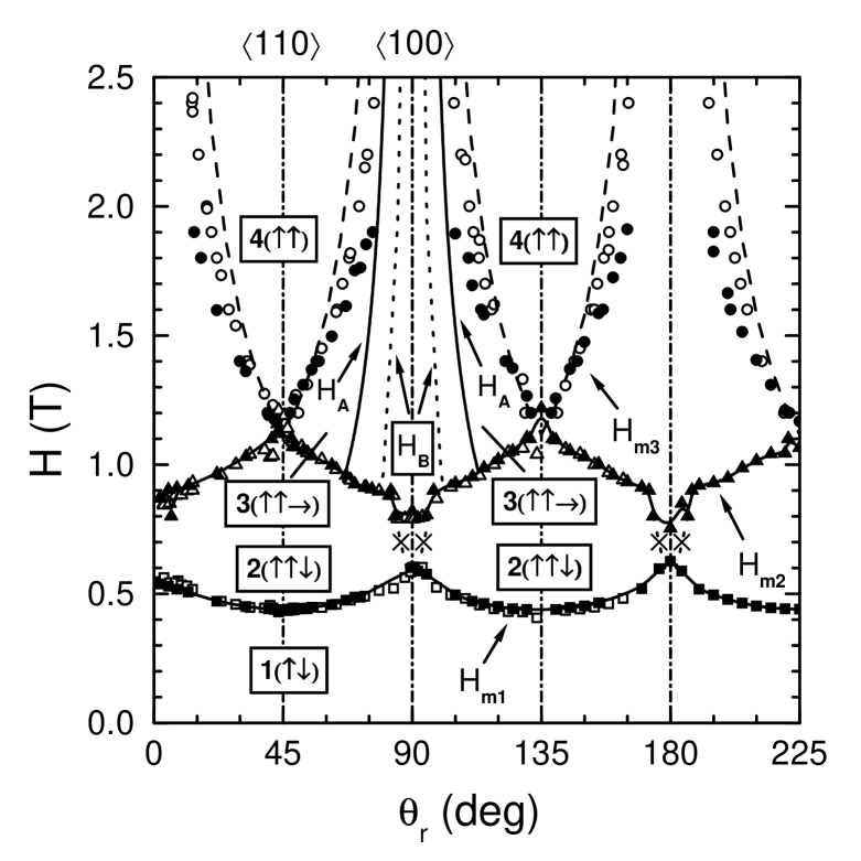
Figure 3: The angular phase diagram of metamagnetic states in HoNi₂B₂C at $T=1.9$ K from torque measurements (increasing field data). $\theta_{r}$ is the angle on the sample rotator. $\theta_{r}=45^{\circ}$, $135^{\circ}$ and $225^{\circ}$ correspond to different $\langle 110\rangle$ easy axes to one degree accuracy. Symbols for different magnetic states are the same as in Fig. 1. $H_{m1}$, $H_{m2}$ and $H_{m3}$ are critical magnetic fields for transitions between different phases. Easy $\langle 110\rangle$ and hard $\langle 100\rangle$ axes are marked in one quadrant. Dashed lines in the upper part represent the theoretical $H_{m3}(\theta)$ dependence (Eq. (3) according to Refs. kalats ; amici ). Solid lines through data for $H_{m1}$ and $H_{m2}$ are guides to the eye. Filled and empty points are obtained with the LM and HM torque chips, respectively. Data points $\times$ represent the extent of frustration region in the ferrimagnetic phase estimated from Fig. 11. Solid and dotted lines ($H_{A}$ and $H_{B}$) shown in only one quadrant correspond to new phase boundaries revealed here (the straight lines A and B in Fig. 1)

.

For the second metamagnetic transition, the models kalats ; amici give the following angular dependence

$$H_{m2}(\phi)=H_{m2}(0)/\cos(\phi),$$ (2)

where $\phi$ is the angle between the field and the nearest hard axis $\langle 100\rangle$ (the line perpendicular to [010] in Fig. 1 represents this relation). In the previous longitudinal magnetization study canf , good agreement with Eq. (2) was found with $H_{m2}(0)=0.84$ T. It also provides a good fit to the data in Fig. 6 (with $H_{m2}(0)=0.88$ T), but only for angles not too close to the hard axis $\langle 100\rangle$, which is the reference axis for this particular transition (see also the corresponding phase-boundary line representing this data in Fig. 1). The peculiar behavior of $H_{m2}$ in the range $-6^{\circ}\lesssim\phi\lesssim 6^{\circ}$ near the hard axis (Fig. 6) will be discussed further below. This contrasts with Ref. canf where good agreement with Eq. (2) was found for all angles except near the easy axis.

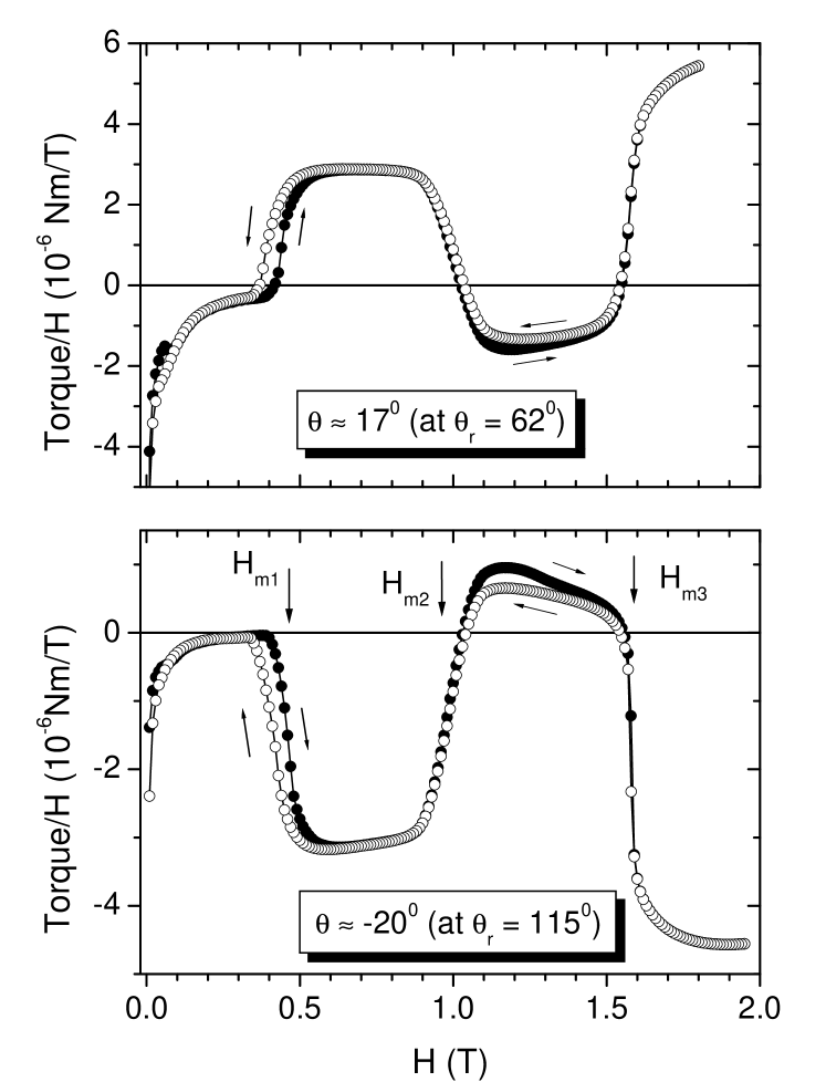
Figure 4: $\tau(H)/H$ curves for angles $\theta\approx 17^{\circ}$ (upper panel) and $\theta\approx-20^{\circ}$ (lower panel) relative to a closest $\langle 110\rangle$ axis (rotator positions in parentheses). Data was recorded for increasing and decreasing magnetic field (arrows) using the LM torque chip. Three metamagnetic transitions ($H_{m1}$, $H_{m2}$ and $H_{m3}$) are marked.

It is emphasized that experimental angular dependences of critical fields for the first two transitions, $H_{m1}(\theta)$ and $H_{m2}(\theta)$, obtained with the LM and HM torque chips are essentially the same (see Figs. 3 and 6). A marked difference between the readings of the LM and HM chips appears only for fields above 1.5 T when the transition to the saturated paramagnetic (ferromagnetic-like) phase at the critical field $H_{m3}$ takes place (Figs. 1 and 3). For this transition the models kalats ; amici give the expression

$$H_{m3}(\phi)=H_{m3}(0)/\sin(\phi).$$ (3)

In Ref. canf a rather good fit to this expression with $H_{m3}(0)=0.66$ T was found (the two solid lines parallel to $\langle 010\rangle$ in Fig. 1). The dashed lines in the upper part of Fig. 3 (drawn for $H_{m3}(0)=0.79$ T) and that in Fig. 1 represent a fit of our data to this equation. It is seen that the agreement can be considered to be satisfactory only for angular positions close to the easy axis (low field region). For angular positions closer to the hard axis, the experimental points deviate more strongly from the prediction of Eq. (3). It is seen that for the HM chip this deviation is much less than for the LM chip in the range 1.5–2.0 T, but above 2 T data from the HM chip deviate significantly as well. This is thought to be mainly due to rotation of the sample and non-linear effects of the cantilever (Sec. II) where angular error can be several degrees. The deviation from the dashed lines in Fig. 1 and Fig. 3 at higher field is to a large extent, but probably not totally, due to these errors.

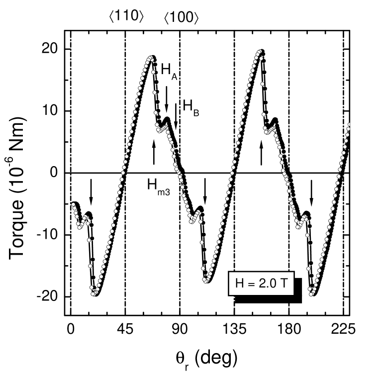
Figure 5: Angular dependence of torque at $H=2.0$ T (HM torque chip). $\theta_{r}$ is the angle on the sample rotator. Easy $\langle 110\rangle$ and hard $\langle 100\rangle$ axes are shown in one quadrant. Filled and empty circles correspond to data for increasing and decreasing angle, respectively. Arrows show angular positions of $H_{m3}$ (transition between ($\uparrow\uparrow\rightarrow$) and ($\uparrow\uparrow$) phases) and fields $H_{A}$ and $H_{B}$ (in one quadrant) for two new phase boundaries (see also Fig.3).

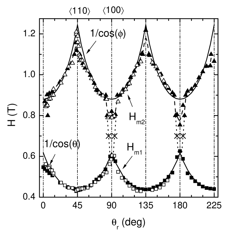
Figure 6: Enlarged portion of Fig. 3 presenting the first two transitions. Solid curve $H_{m1}$ represents $H_{m1}(\theta)=H_{m1}(0)/\cos(\theta)$ with $H_{m1}(0)=0.437$ T for the [($\uparrow\downarrow$)–($\uparrow\uparrow\downarrow$)] transition ($\theta$ is the angle between the field and the nearest easy axis). Curve $H_{m2}$ represents $H_{m2}(\theta)=H_{m2}(0)/\cos(\phi)$ with $H_{m2}(0)=0.88$ T for the [($\uparrow\uparrow\downarrow$)–($\uparrow\uparrow\rightarrow$)] transition ($\phi$ is the angle between field and nearest hard axis). Symbols are the same as in Fig. 3.

Some general comments regarding the angular phase diagram for metamagnetic states in HoNi₂B₂C obtained in this study can be made. First, the diagram in Fig. 3 appears to be quite periodic (with a period of $90^{\circ}$). This implies, that low-temperature orthorhombic distortions of the tetragonal lattice of HoNi₂B₂C, found in Ref. kreysig , do not cause an appreciable disturbance of angular symmetry of the metamagnetic transitions. It cannot be ruled out, however, that the orthorhombic distortions can cause corresponding distortions in magnetic order of the metamagnetic states muller ; kreysig . Possible indications of these effects in the results obtained will be considered in more detail below in the discussion of particular features of the metamagnetic states (Sec. III.2). Second, according to Ref. canf , for magnetic field directions close to a $\langle 110\rangle$ axis ($-6^{\circ}\lesssim\theta\lesssim 6^{\circ}$), solely the ($\uparrow\downarrow$)–($\uparrow\uparrow\downarrow$)–($\uparrow\uparrow$) sequence with only two transitions ($H_{m1}$, $H_{m2}$) is observed (see solid lines in Fig. 1). In this sequence, the transition to the non-collinear ($\uparrow\uparrow\rightarrow$) phase is not present. In contrast, one model amici indicates that this sequence of two transitions is possible at $\theta=0$ only. Analysis of the magnetic-field dependences of the torque for different angles, including angles close to $\theta=0$, indicates that the angular range for this sequence of only two metamagnetic transitions ($H_{m1}$, $H_{m2}$) is only $|\theta|<1^{\circ}$, far less than that indicated in canf (compare the phase boundaries from data of the two studies in Fig. 1), i.e., the torque measurements for the angles $|\theta|\geq 1^{\circ}$ showed three transitions $H_{m1}$, $H_{m2}$ and $H_{m3}$. Thus, torque results support the assertion in amici that the sequence of transitions ($\uparrow\downarrow$)–($\uparrow\uparrow\downarrow$)–($\uparrow\uparrow$) occurs only for $\theta=0$.

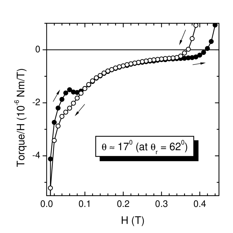
Figure 7: $\tau(H)/H$ dependence at $\theta\approx 17^{\circ}$ ($\theta_{r}=62^{\circ}$). Filled and empty circles indicate increasing and decreasing field, respectively.

III.2 Remarkable features of the metamagnetic states

In this subsection some surprising features of the metamagnetic states and transitions in HoNi₂B₂C are considered. First, the net magnetization of the AFM phase must be equal to zero, and the same should be expected for the torque (magnetic field less than $H_{m1}$). The experimental evidence is inconsistent with this. In Fig. 4, the magnetic-field dependence of the torque (divided by field), $\tau(H)/H=M\sin(\beta)$, is shown for two angles $\theta_{r}$. A blow-up for one of the angles is shown in Fig. 7. The $\tau(H)/H$ magnitude is non-zero below $H_{m1}$, but approaches zero just below $H_{m1}$. Also, $\tau(H)/H$ is hysteretic in the region $H<0.1$ T, but above this up to $H_{m1}$ the curves for increasing and decreasing field coincide. Such dependences, with $\tau(H)/H$ being negative below $H_{m1}$, are found for most of the angular range for angles $\theta$ of either sign (compare $\tau(H)/H$ curves in Fig. 4 for $\theta\approx 17^{\circ}$ and $\theta\approx-20^{\circ}$). Only on the margins of the range investigated ($0\lesssim\theta_{r}\lesssim 25^{\circ}$ and $180^{\circ}\lesssim\theta_{r}\lesssim 230^{\circ}$) are the $\tau(H)/H$ values positive below $H_{m1}$ (see upper panel of Fig. 8), but all other features are the same. Generally, the modulus of $\tau(H)/H$ approaches zero with increasing field before the first transition starts (Figs. 4, 7 and 8). Opposite signs for $\tau(H)/H$ in different angular ranges may be an indication of non-equivalence of easy axes $\langle 110\rangle$ (at least for the AFM state).

The non-zero absolute value of $\tau(H)/H=M\sin(\beta)$ implies that $M\neq 0$ as well. This may be possible for the AFM state if a multidomain AFM structure exists. This can be justified by availability of four (or at least two) equivalent easy $\langle 110\rangle$ directions in HoNi₂B₂C, as described above. In such case, on cooling below the Néel temperature domains can easily appear morrish . The low-temperature orthorhombic distortions facilitate this process since a shortening of the crystal lattice can take place along the $\langle 110\rangle$ directions in which the moments align kreysig . When a multidomain (or, most likely, two-domain) AFM structure exists, the magnetic moments of the domains may not be completely compensated, and the torque may be non-zero. The decrease of torque to nearly zero with increasing field suggests a transformation to a one-domain state.

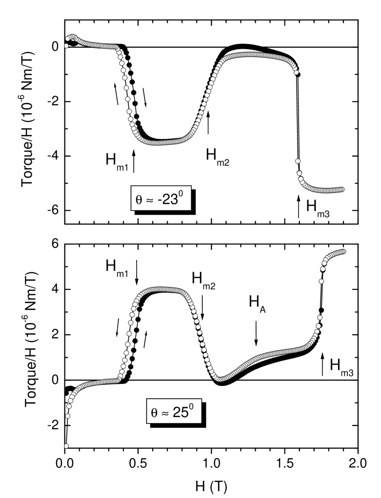
Figure 8: The magnetic-field dependence of torque (divided by field) for angles close to predicted direction for magnetization in the $\uparrow\uparrow\rightarrow$ phase $\theta\approx-23^{\circ}$ (upper panel) and $\theta\approx 25^{\circ}$ (lower panel) relative to the closest $\langle 110\rangle$ axis (rotator angle in parentheses). Data for increasing and decreasing field (arrows) was taken with the LM piezoresistive chip. Critical fields $H_{m1}$, $H_{m2}$, $H_{m3}$ and $H_{A}$ are indicated by arrows.

It should be mentioned that the upper critical field $H_{c2}$ for HoNi₂B₂C is about 0.3 T at $T=2$ K daya ; lin . Thus, the torque hysteresis in the AFM phase is in the superconducting state. Therefore, the non-zero torque and hysteresis in the low-field range of the AFM state (Fig. 7) may also be related to trapped flux generated on passing through the critical field, both as $H$ is increased and decreased. (Note: data is taken as the field is increased and decreased at a fixed angle. The angle is then changed to the next value at approximately zero field, still at 1.9 K.) In Ref. lin , a noticeable hysteresis in the magnetization at $T=2$ K in polycrystalline HoNi₂B₂C was found at $H<0.1$ T, which is consistent with the torque behavior found in this study. Recent Bitter decoration experiments vinnik indicate the possibility that pinned vortex structures could be important in the AFM phase. They suggest that the pinning may arise from AFM twin magnetic grain boundaries which supports the argument that multidomain effects explain these low field non-zero torques in the AFM phase.

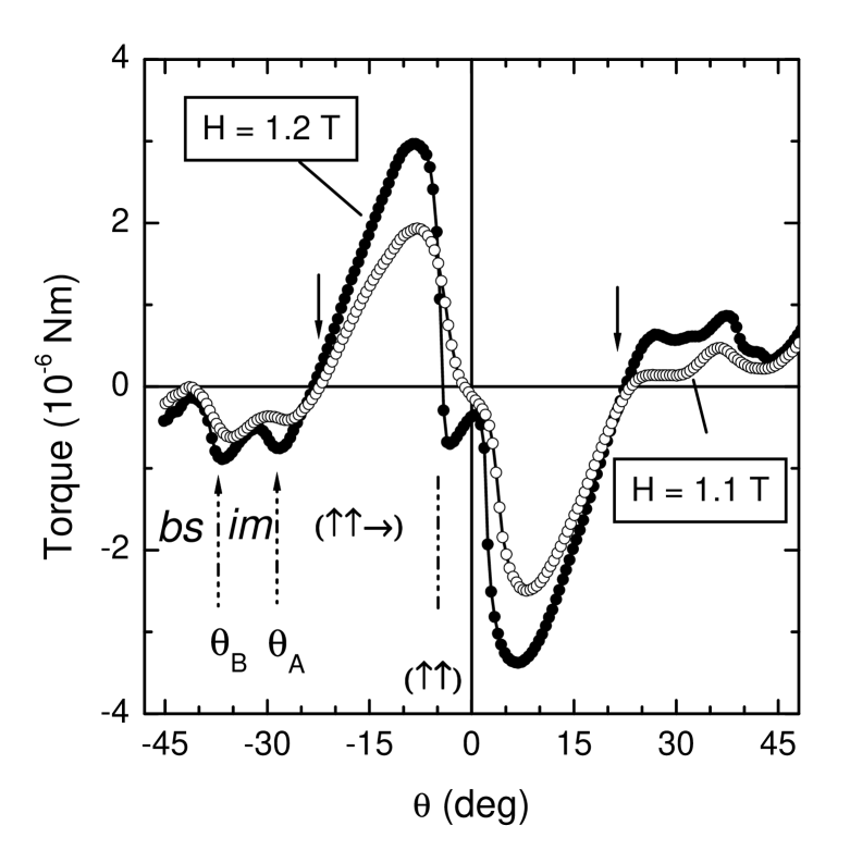
Figure 9: Angular dependence (increasing angle) of the torque at $H=1.1$ T and $H=1.2$ T with the LM chip. With increasing $\theta$ (angle to a closest $\langle 110\rangle$ axis) torque changes abruptly for the metamagnetic transition between the ($\uparrow\uparrow\rightarrow$) and ($\uparrow\uparrow$) phases (near $\theta\approx 3^{\circ}$ and $\theta\approx-3^{\circ}$ for $H=1.2$ T). Generally, with increasing $\theta$ the sequence of transitions, ($\uparrow\uparrow$)–($\uparrow\uparrow\rightarrow$)–(intermediate state)–(border state), occurs (symbols $\it im$ and $\it bs$ represent the last two phases discussed in the main text). Zero crossing of torque at $|\theta|\approx 23^{\circ}$ (vertical arrows) indicates the direction of $\vec{M}$ in the non-collinear ($\uparrow\uparrow\rightarrow$) phase.

The transition, from the ferrimagnetic ($\uparrow\uparrow\downarrow$) to the non-collinear ($\uparrow\uparrow\rightarrow$) state, at $H=H_{m2}$ is rather broad, but with negligible hysteresis (Figs. 4 and 8). According to the model kalats , the magnetization in the phase ($\uparrow\uparrow\rightarrow$) is tilted by an angle $\Phi=\arctan(1/2)\approx 26.6^{\circ}$ to the easy $\langle 110\rangle$ axis closest to the magnetic field, and its absolute value is equal to $\approx 0.745$ of the easy-axis saturation value. Thus, not only does a change in magnetization magnitude take place at this transition, but also the angle between the magnetization and applied field changes. For the torque $\vec{\tau}=\vec{M}\times\vec{H}$ with the modulus $\tau=MH\sin(\beta)$, this implies that the angle $\beta$ will be changed $26.6^{\circ}$ at this transition. The angles $\beta$ and $\theta$ can be taken as identical in the ferrimagnetic phase. Thus relation $\beta=\theta-\Phi$ should hold after transition to the non-collinear phase. This is verified very well in this torque study. A change in sign of the torque at the transition is expected for field directions, for which $|\theta|<\Phi$ and is found (Fig. 4). Also the torque must be close to zero after the transition for $\theta\approx\Phi$. This specific case is also confirmed (Fig. 8). Since the torque changes sign as $\beta$ changes sign when $\theta=\Phi$ in the field range for existence of the ($\uparrow\uparrow\rightarrow$) phase, $\Phi$ can be precisely determined from the angular dependence of the torque. Figure 9 presents such dependences for fields 1.1 T and 1.2 T. For both fields a change in sign of the torque occurs at $\theta\approx 23^{\circ}$, which is close to but smaller than the theoretical value of $\Phi$. For fields $H=1.4$ T and 1.5 T this angle is about $22^{\circ}$ and $20^{\circ}$, respectively, suggesting that $\Phi$ depends on the applied field.

As mentioned above, it is possible, using the angles $\beta$ for each phase as described above, to calculate the magnetization magnitude for different metamagnetic states of the sample by dividing the torque measured in the range of each phase by $H\sin(\beta)$. The results are: 1) $M_{\uparrow\uparrow\downarrow}=(0.9-0.95)\times 10^{-2}$ emu (for the ferrimagnetic phase); 2) $M_{\uparrow\uparrow\rightarrow}\simeq 1.8\times 10^{-2}$ emu (for the non-collinear phase at $H=1.6$ T); 3) $M_{\uparrow\uparrow}\simeq 2.8\times 10^{-2}$ emu (for the ferromagnetic-like phase at $H=1.6$ T). It is seen that $M_{\uparrow\uparrow}/M_{\uparrow\uparrow\downarrow}\approx 3$ in line with the model kalats . The ratio $M_{\uparrow\uparrow\rightarrow}/M_{\uparrow\uparrow}$ is about 0.64 according to our estimates. This is somewhat less than that (0.745) predicted by the model kalats . It should be noted, however, that 0.745 is expected only together with $\Phi=26.6^{\circ}$. For a smaller $\Phi$, the magnetization of the non-collinear phase should be smaller, so that a somewhat diminished ratio $M_{\uparrow\uparrow\rightarrow}/M_{\uparrow\uparrow}$ is quite expected. Furthermore, there is no reason to expect that the simple model kalats ; amici which assumes only ferromagnetic coupling of the $ab$-planes would predict $\Phi$ (or $M_{\uparrow\uparrow\rightarrow}$) precisely when the modulation vector measured by neutron scattering camp ; detlef ; schneider is $q\approx 0.58$ $a^{*}$, not $q=2/3$ $c^{*}$ as predicted for the ($\uparrow\uparrow\rightarrow$) phase kalats ; amici .

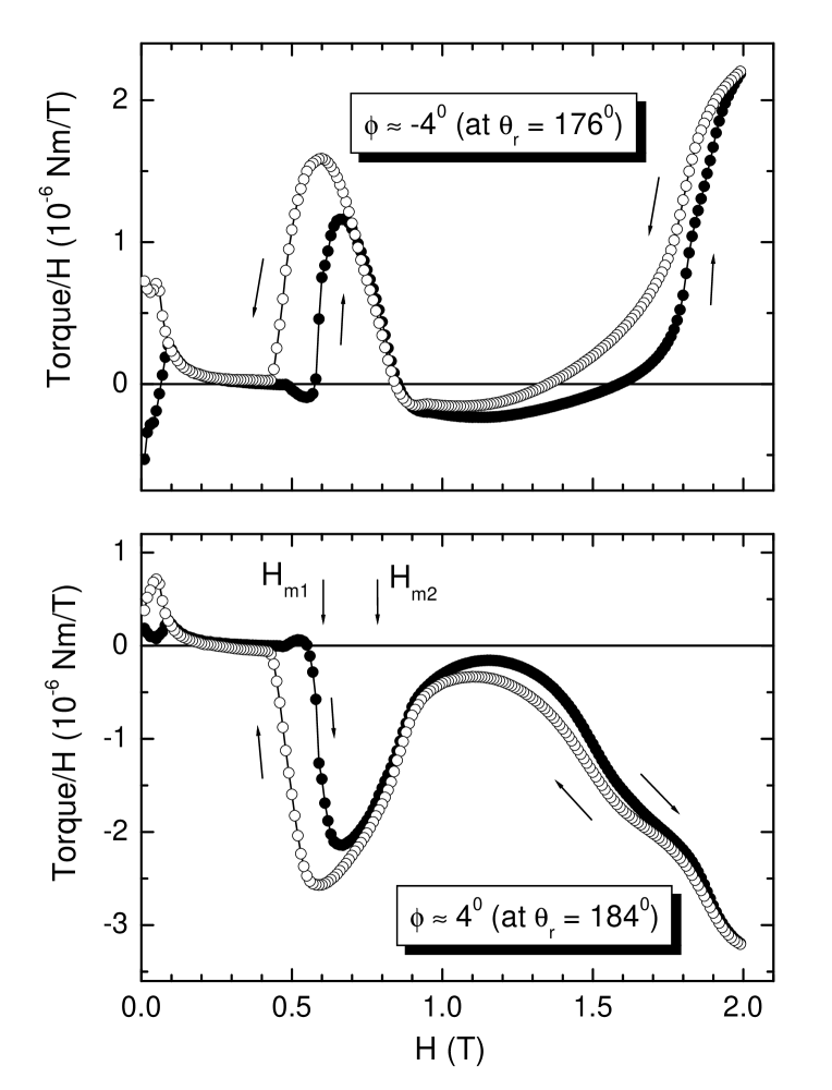
Figure 10: Dependences $\tau(H)/H$ for increasing and decreasing field (arrows) for angles $\phi\approx-4^{\circ}$ (upper panel) and $\phi\approx 4^{\circ}$ (lower panel) relative to the closest $\langle 100\rangle$ hard axis (rotator angles in parentheses). The metamagnetic transitions ($\uparrow\downarrow$)–($\uparrow\uparrow\downarrow$) and ($\uparrow\uparrow\downarrow$)–($\uparrow\uparrow\rightarrow$) at $H_{m1}$ and $H_{m2}$ for angles $\phi$ near 0 are quite close together, indicative of frustrated behavior.

As mentioned earlier, the angular behavior of $H_{m2}$ for angles very close to the hard axis $\langle 100\rangle$ ($-6^{\circ}\lesssim\phi\lesssim 6^{\circ}$) deduced from the torque measurements is not described by Eq. (2). The $H_{m2}$ values in this region are far below those predicted by Eq. (2) (Figs. 3 and 6). Behavior of $\tau(H)/H$ for small values of $\phi$ is shown in Fig. 10 to help understand this phenomenon. It can be seen that the magnetic-field behavior of the torque in the AFM state is similar to that for angles $\phi$ far from zero (compare Fig. 10 with Figs. 4, 7, and 8). The first transition to the ferrimagnetic state manifests itself quite clearly, although with larger hysteresis. With a further increase in field the system behaves rather peculiarly: the first ($\uparrow\downarrow$)–($\uparrow\uparrow\downarrow$) and the second ($\uparrow\uparrow\downarrow$)–($\uparrow\uparrow\rightarrow$) metamagnetic transitions are much closer together for small $\phi$ than expected. The phase boundaries may not really be changed, but the system cannot decide which direction its magnetization should point, to the left or to the right of the hard axis. This behavior of the magnetic system studied for small $\phi$ is characteristic of “frustration”.

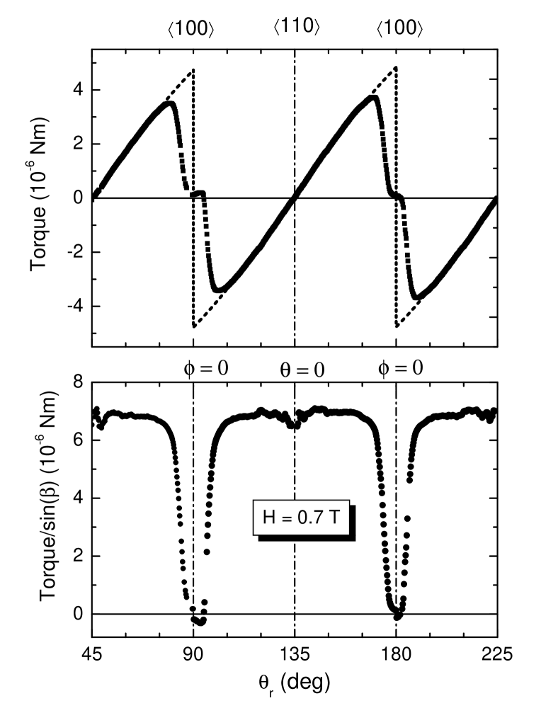
Figure 11: Angular dependence of torque for increasing angle with the LM piezoresistive chip (upper panel) and $\tau/\sin(\beta)$ (lower panel) at $H=0.7$ T where only the ferrimagnetic ($\uparrow\uparrow\downarrow$) phase exists and $\beta=\theta$ ($\theta_{r}$ is angular position of the rotator). Easy $\langle 110\rangle$ and hard $\langle 100\rangle$ axes with the corresponding values $\theta=0$ and $\phi=0$, are shown. The dashed line indicates the expected dependence of torque near $\phi=0$ upon the change from one ferrimagnetic state ($\uparrow\uparrow\downarrow$) to another ($\rightarrow\rightarrow\leftarrow$). The extent of the frustrated region in the ferrimagnetic state is indicated by the region of almost zero torque near $\phi=0$.

Additional important features of “frustration” near $\phi=0$ were found in the angular dependences of the torque. Figures 5, 11 and 12 reveal that the torque goes to zero as the direction of the magnetic field approaches $\phi=0$ from any side in the angular region of the ferrimagnetic ($\uparrow\uparrow\downarrow$) and non-collinear ($\uparrow\uparrow\rightarrow$) phases (see the phase diagram in Fig. 3). This behavior of the torque is in sharp contrast to the simple picture expected from the models kalats ; amici where the component of the magnetization normal to the hard axis changes sign as the field direction crosses $\phi=0$. Therefore, $\sin(\beta)$ is expected to change sign as well on crossing the angle $\phi=0$, producing a very sharp jump in the torque at $\phi=0$ as depicted by dashed lines in Figs. 11 and 12. The experimental picture is far from that (compare the experimental and calculated curves in these figures).

It is possible, in principle, to derive angular dependences of the magnetization (including the “frustrated” region near $\phi=0$) from the corresponding angular dependences of the torque, if the angle $\beta$ is known for all $\theta$. In this case the values of $\tau/\sin(\beta)$, which should be proportional to the magnetization, can be calculated. The angular dependence of $\tau/\sin(\beta)$ for $H=0.7$ T, calculated with the assumption $\beta=\theta$, is shown in Fig. 11. It is seen that $\tau/\sin(\beta)$ goes to zero when approaching $\phi=0$. This takes place approximately in the range $-6^{\circ}\lesssim\phi\lesssim 6^{\circ}$. Outside these regions, $\tau/\sin(\beta)$ is approximately constant as expected for the ($\uparrow\uparrow\downarrow$) phase.

Thus, for the ferrimagnetic phase “frustration” proceeds in a rather narrow angular range $-6^{\circ}\lesssim\phi\lesssim 6^{\circ}$. This range is estimated by the dotted lines through the data points $\times$ in Fig. 6. It can be suggested that, for the ferrimagnetic ($\uparrow\uparrow\downarrow$) phase near the hard axis, a border state develops where $\tau\rightarrow 0$ as $\phi\rightarrow 0$. When the angular position of the field crosses the hard axis, ordered moments change their alignment from one easy axis to another. So that this transition should be accompanied by considerable magnetoelastic deformation or a change in direction of the orthorhombic distortion, therefore, being actually first order. The increased angular hysteresis in the vicinity of a hard axis, mentioned above in Sec. III.1, supports this view.

Although Fig. 11 could be interpreted as $M\rightarrow 0$ as $\phi\rightarrow 0$, that is inconsistent with longitudinal magnetization measurements daya ; schneider . It is more likely that $\sin(\beta)$ goes to zero as the field direction crosses the angle $\phi=0$. In such an event, the magnetization at $\phi=0$ can be non-zero, but the average magnetization of the sample should be directed along the hard axis $\langle 100\rangle$ with $\beta=0$.

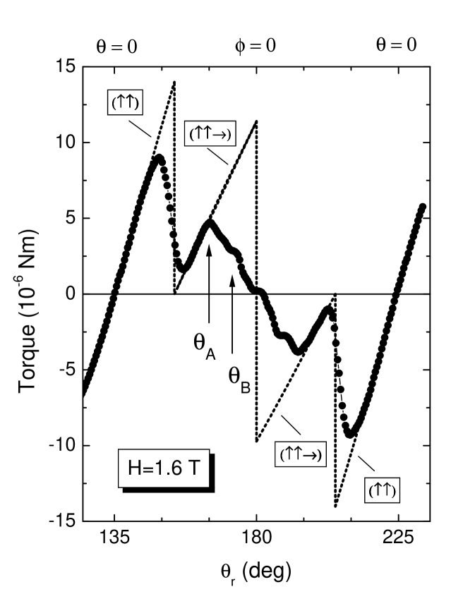
Figure 12: Angular dependence of torque at $H=1.6$ T [HM chip, $\theta_{r}$ rotator angle, easy $\langle 110\rangle$ ($\theta=0$) and hard $\langle 100\rangle$ ($\phi=0$) axes]. Filled and empty circles represent increasing and decreasing angle, respectively. Dashed lines show the expected angular dependence of the torque in the angular areas of the ferromagnetic-like ($\uparrow\uparrow$) and non-collinear ($\uparrow\uparrow\rightarrow$) phases with $\beta=\theta$ for the ($\uparrow\uparrow$) phase and $\beta=\theta-\Phi$ for the ($\uparrow\uparrow\rightarrow$) phase over the predicted range of these phases ($\beta$ is the angle between the field and the magnetization, $\Phi$ is the predicted angle kalats ; amici between magnetization and an easy axis in the $\uparrow\uparrow\rightarrow$ phase). $\theta_{A}$ and $\theta_{B}$ indicate positions of drastic changes in the torque corresponding to two new phase boundaries represented by the lines A and B in Fig. 1. Note increased angular hysteresis near the hard axis in the region of these two phases.

Frustration takes place in two steps in the non-collinear phase. When $\theta$ increases above some specific angle $\theta_{A}$ (defined as a position of the maximum in $\tau(\theta)$ in the region of the ($\uparrow\uparrow\rightarrow$) phase in Fig. 12) the torque decreases rather steeply to a plateau. At somewhat larger angle it decreases rapidly again at $\theta_{B}$ to a second plateau near zero torque. It is significant that deviation of torque behavior from that expected (in line with models kalats ; amici ) for the non-collinear phase begins well away from $\phi=0$ (Fig. 12). So it appears that, in some substantial angular range around the hard axis, the metamagnetic state of the sample is different from the non-collinear phase described in models kalats ; amici . Due to the radical change in angular behavior of the torque at the angle $\theta_{A}$ we can consider this point as an indication of a new metamagnetic transition from the non-collinear ($\uparrow\uparrow\rightarrow$) phase to a different phase which we will call the intermediate state. The critical angle $\theta_{A}$ for this transition is found to be strongly field dependent ranging, when measured from a hard axis, from about $24^{\circ}$ at $H=1.0$ T to about $4^{\circ}$ at $H=3.2$ T. The corresponding phase boundary is represented by a straight line A in Fig. 1 which is parallel to the dashed straight line of the ($\uparrow\uparrow\rightarrow$)-($\uparrow\uparrow$) transition plotted according to models kalats ; amici . Therefore, the critical field $H_{A}$, defined by line A in Fig. 1, has the same $1/sin(\phi)$ angular dependence as that given by Eq. (3). The field $H_{A}(\phi=0)\approx 0.35$ T is roughly one-half of the field $H_{m3}(0)\approx 0.79$ T. The solid line corresponding to this boundary $H_{A}$ is shown also in the angular phase diagram in Fig. 3.

The second specific angle $\theta_{B}$ shown in Fig. 12 is strongly field dependent as well, defining another transition to a new metamagnetic state which will be called the border state. The transition indicated by the angle $\theta_{B}$ is represented by the line B in Fig. 1 and the corresponding critical field $H_{B}$ is also found to be proportional to $1/\sin(\phi)$ as in Eq. (3) with $H_{B}(0)\approx 0.17$ T, almost exactly one-half of $H_{A}(0)$. It can be suggested, therefore, that Figure 12 shows the following sequence of transitions with increasing $\theta$ from 0 to $45^{\circ}$: ($\uparrow\uparrow$)–($\uparrow\uparrow\rightarrow$)–(intermediate state)–(border state). According to the phase diagram in Fig. 1, this sequence of transitions should take place for any field above $\simeq 1.1$ T (but, of course, with other critical angles). Indeed, $\theta_{A}$ and $\theta_{B}$ can be seen in Figs. 5 and 9, too.

The occurrence of the intermediate phase was found at first by means of examination of angular dependences of torque like those shown in Figs. 5, 9 and 12. The resulting phase diagram (Fig. 1) implies, however, that this phase should manifest itself in experimental $\tau(H)$ curves as well for some rather narrow angular range which was estimated to be $24^{\circ}\leq\theta\leq 32^{\circ}$. Within this range the following sequence of metamagnetic transitions is expected with increasing field: ($\uparrow\downarrow$)–($\uparrow\uparrow\downarrow$)–(intermediate phase)–($\uparrow\uparrow\rightarrow$)–($\uparrow\uparrow$). For angles $\theta$ smaller than $\approx 24^{\circ}$ only three transitions should occur: ($\uparrow\downarrow$)–($\uparrow\uparrow\downarrow$)–($\uparrow\uparrow\rightarrow$)–($\uparrow\uparrow$). Both these cases are apparent in Fig. 8. In the upper panel, $\tau(H)/H$ is presented for angle $\theta\approx-23^{\circ}$ (which is equivalent to $\theta\approx 23^{\circ}$ due to the angular symmetry). The magnitude of $\tau(H)/H$ at a constant angle $\theta$ is equal to the normal component of the magnetization. It is seen that when transition with critical field $H=H_{m2}$ is completed for high enough field, the magnetization is nearly constant for $\theta\approx-23^{\circ}$; whereas, for $\theta\approx 25^{\circ}$, the magnetization first increases with increasing field and only for a higher field the magnetization appears to come to a saturated value. This is where the transition between the intermediate and the non-collinear phases is expected according to the line A in Fig. 1. This transition manifests itself more clearly for higher angles $\theta$ (not shown).

We have defined the transition lines A and B in Fig. 1 based on distinct features in the torque vs. $\theta$ curves at constant field, but there is uncertainty in the exact part of the feature that represents the transition. The experimental angular uncertainty is also more important in this small angular range. Nevertheless, the $1/\sin(\phi)$ dependence for $H_{A,B}$ in Figs. 1 and 3 is quite precise, though the “actual” transition could be shifted parallel to the hard axis slightly in Fig. 1. Based on the arguments used by Canfield et al. canf , the $1/\sin(\phi)$ dependence implies that the change in magnetization $\Delta\vec{M}$ at these boundaries (lines A and B) is normal to the nearest hard axis from the field direction. Thus $|\Delta\vec{M}|=\Delta\tau\tan(\phi)/H_{A}(0)$ where $\Delta\tau$ is the change in torque at the boundary A. With $\Delta\tau$ from torque vs. $\theta_{r}$ data at fixed $H=1.3$ T and 1.4 T (not shown, but like that shown in Fig. 9 for $H=1.1$ and 1.2 T and Fig. 12 for $H=1.6$ T), we estimate $|\Delta M|\approx 4\times 10^{-3}$ emu. Under the assumption that $M_{\uparrow\uparrow}\approx 2.8\times 10^{-2}$ emu corresponds to 9.8 $\mu_{B}$ per Ho ion, this $|\Delta M|$ corresponds very roughly to flipping one Ho³⁺ moment in 6 of those aligned along the nearest easy axis to the applied field $\vec{H}$ to the perpendicular easy axis in going from the non-collinear phase ($\uparrow\uparrow\rightarrow$) to the intermediate state. Although the error is much larger since the B line can be intercepted only with $\vec{H}$ less than $10^{\circ}$ from the hard axis, a similar estimate indicates very roughly that an additional 2 in 9 Ho³⁺ moments originally along the dominant easy axis are flipped $90^{\circ}$ in going from the intermediate state to the border state.

Can the available neutron scattering data for HoNi₂B₂C detlef ; camp ; schneider clarify the new results of this torque study, concerning new phase boundaries revealed and “frustration” behavior near a hard axis? Data by Detlefs, et al. detlef at $15^{\circ}$ to the easy axis shows the $q\approx 0.58$ $a^{*}$ modulation vector in the region of the ($\uparrow\uparrow\rightarrow$) phase in Fig. 3 while that by Campbell, et al. camp along the hard axis in the region of the border phase shows a $q\approx 0.61$ $a^{*}$ modulation vector. Measurements by Schneider schneider with increasing field along the hard axis (in the $b^{*}$-direction) at 2 K indicate the presence of a $0.58$ $a^{*}$ propagation vector in the ferrimagnetic phase which switches over to a 0.62 $b^{*}$ propagation vector (parallel to the applied field) in coexistence with a weaker 0.60 $b^{*}$ modulation in the region of our “border” phase. He suggests, based on the argument detlef that the $a^{*}$, $b^{*}$ modulations may only develop from non-collinear phases, that the 0.58 $a^{*}$ modulation in the ferrimagnetic phase region may be associated with the C6 non-collinear phase $(\uparrow\downarrow\uparrow\rightarrow\leftarrow\rightarrow)$ predicted by Amici and Thalmeier amici . We note that this phase with magnetization along the hard axis might possibly develop in the very narrow frustration region near the hard axis in the ferrimagnetic phase (see Fig. 11), but we did not see any evidence of a phase boundary in the entire ferrimagnetic region corresponding to that predicted for C6 amici , and the torque measurements outside of the frustration region were completely consistent with the ($\uparrow\uparrow\rightarrow$) phase, as were longitudinal magnetization measurements daya ; schneider . We note that the boundary between our “intermediate” phase and the non-collinear phase is in the general vicinity of the F2 phase ($\uparrow\rightarrow$) predicted by Amici and Thalmeier amici , but the field-angle dependence is quite different. We can only speculate that the $b^{*}$-modulations observed by Schneider may be related to the “border” and “intermediate” phases observed here.

It is also possible that the “frustration” behavior results from a two-domain state when two possible directions of orthorhombic distortions are realized simultaneously when the field is directed close enough to the hard axis (so that there is some mixed state around the hard axis rather than a single phase). The magnetization that determines the torque is the total magnetization which, in that scenario, can lie close to $\phi=0$, though the Ho moments lie only along easy directions locally. We have found, that in these two new (intermediate and border) phases, the net magnetization appears to rotate in steps toward the hard axis as the applied field is rotated toward that direction, suggesting that they may both be states consisting of mixture of two or more phases in a ratio that changes with applied field. The discovery of “frustration” in the magnetic phases of HoNi₂B₂C for the field direction along the hard axis $\langle 100\rangle$ is an important new result of the present study.

The new phenomena found in this study raises the question: why were they not revealed in the longitudinal magnetization measurements canf ? Obvious reasons may be insensitivity to the component of $\vec{M}$ normal to the field and the rather large error bars for orientation of the field in the $ab$-plane of HoNi₂B₂C crystal lattice, which in Ref. canf were about $\pm 4^{\circ}$. In the present study this error is far less ($\pm 1^{\circ}$), but the main advantages of torque magnetometry are that the relative angular accuracy (when rotating a sample consistently in only one direction) is very high and that it is very sensitive to the normal component of $\vec{M}$ which is subject to fluctuations near $\phi=0$. The data obtained show quite consistent, not random changes in the torque magnitude for angle variations about 0.25^∘ or even less. As a result, the angular torque dependences consist of hundreds of points that allow detection of important features of the torque angular behavior.

IV Conclusions

These torque measurements provide not only a check of the known results and refinement of the angular diagram for metamagnetic transitions in HoNi₂B₂C, but also clarify some important features of these metamagnetic states and, moreover, indicate new states. Indications of a magnetically inhomogeneous state of the AFM phase at low magnetic field, which is likely determined by a combined influence of multidomain magnetic structure and flux trapping in the superconducting state were found. The first precise determination of the magnetization direction in the ($\uparrow\uparrow\rightarrow$) phase was made. This direction varies with the magnitude of the applied field which does not agree with model predictions kalats ; amici . Two new phase boundaries parallel to the hard axis in the $ab$-plane polar field plot (Fig. 1) were indicated in a region previously ascribed to the non-collinear ($a^{*}$ or $b^{*}$ modulated) phase. “Frustration” was observed when the direction of magnetic field is close to the hard axis $\langle 100\rangle$ ($-6^{\circ}\lesssim\theta\lesssim 6^{\circ}$) and tentatively explained by a mixed (two-domain) state of the system with moments aligned along different equivalent easy axes. These torque magnetometry measurements indicate a more complicated magnetic behavior and suggest important parts of the phase diagram where more detailed neutron scattering measurements should be focussed.

- (1) D. G. Naugle, K. D. D. Rathnayaka, and A. K. Bhatnagar, in Studies of High Temperature Superconductors, edited by A. Narlikar (Nova Science Publishers, Commack, NY, 1999), Vol. 28, pp. 199-239.
- (2) K.-H. Müller and V. N. Narozhnyi, Rep. Progr. Phys. 64, 943 (2001).
- (3) P. Thalmeier and G. Zwicknagl, in ”Handbook on the Physics and Chemistry of Rare Earths” edited by Karl A. Gschneidner (Elsevier, Amsterdam, 2005), Vol. 34, Chap. 219, p. 135; also in preprint cond-mat/0312540.
- (4) L. C. Gupta, Adv. Phys. 55, 691 (2006).
- (5) T. Siegrist, H. W. Zandbergen, R. J. Cava, J. J. Kraevski, and W. F. Peck, Jr., Nature 67, 254 (1994).
- (6) J. W. Lynn, S. Skanthakumar, Q. Huang, S. K. Sinha, Z. Hossain, L. C. Gupta, R. Nagarajan, and C. Godart, Phys. Rev. B 55, 6584 (1997).
- (7) K. Winzer, K. Krug, and Z. Q. Peng, J. Magn. Magn. Mater. 226-230, 321 (2001).
- (8) P. C. Canfield, S. L. Bud’ko, B. K. Cho, A. Lacerda, D. Farrell, E. Johnston-Halperin, V. A. Kalatsky, and V. L. Pokrovsky, Phys. Rev. B 55, 970 (1997).
- (9) K. D. D. Rathnayaka, D. G. Naugle, B. K. Cho, and P. C. Canfield, Phys. Rev. B 53, 5688 (1996).
- (10) V. A. Kalatsky and V. L. Pokrovsky, Phys. Rev. B 57, 5485 (1998).
- (11) A. Amici and P. Thalmeier, Phys. Rev. B 57, 10684 (1998).
- (12) Tuson Park, M. B. Salamon, Eun Mi Choi, Heon Jung Kim, and Sung-Ik Lee, Phys. Rev. B 69, 054505 (2004).
- (13) A. J. Campbell, D. McK. Paul, and G. J. McIntyre, Phys. Rev. B 61, 5872 (2000)
- (14) C. Detlefs, F. Bourdarot, P. Burlet, P. Dervenagas, S. L. Bud’ko, and P. C. Canfield, Phys. Rev. B 61, R14916 (2000).
- (15) M. Schneider, Ph. D. thesis, Swiss Federal Institute of Technology, Zurich, 2006. Available at http://e-collection.ethbib.ethz.ch/show?type=diss&nr=16493.
- (16) C. Sierks, M. Doerr, A. Kreysig, M. Loewenhaupt, Z. Q. Peng, and K. Winzer, J. Magn. Magn. Mater. 192, 473 (1999).
- (17) A. Kreyssig, M. Loewenhaupt, J. Freudenberger, K.-H. Müller, and C. Ritter, J. Appl. Phys. 85, 6058 (1999).
- (18) Ming Xu, P. C. Canfield, J. E. Ostenson, D. K. Finnemore, B. K. Cho, Z. R. Wang, D. C. Johnston, Physica C 227, 321 (1994).
- (19) M. Willemin, C. Rossel, J. Brugger, M. H. Despont, H. Rothuizen, P. Vettiger, J. Hofer, and H. Keller, J. Appl. Phys. 83, 1163 (1998).
- (20) Neil Dilley (Quantum Design), private communication.
- (21) Allan H. Morrish, “The Physical Principles of Magnetism” (John Wiley & Sons, NY, 1965).
- (22) M. S. Lin, J. H. Shieh, Y. B. You, W. Y. Guan, H. C. Ku, H. D. Yang, and J. C. Ho, Phys. Rev. B 52, 1181 (1995).
- (23) L. Ya. Vinnikov, J. Anderegg, S. L. Bud’ko, P. C. Canfield, and V. G. Kogan, Phys. Rev. B 71, 224513 (2005).