The Thermal Composite Supernova Remnant Kesteven 27 as Viewed by CHANDRA: Shock Reflection from a Cavity Wall

Abstract

We present a spatially resolved spectroscopic study of the thermal composite supernova remnant Kes 27 with Chandra. The X-ray spectrum of Kes 27 is characterized by K lines from Mg, Si, S, Ar, and Ca. The X-ray–emitting gas is found to be enriched in sulfur and calcium. The broadband and tricolor images show two incomplete shell-like features in the northeastern half and brightness fading with increasing radius to the southwest. There are over 30 unresolved sources within the remnant. None shows characteristics typical of a young neutron star. The maximum diffuse X-ray intensity coincides with a radio-bright region along the eastern border. In general, gas in the inner region is at higher temperature, and the emission is brighter, than that in the outer region. The gas in the remnant appears to be near ionization equilibrium. The overall morphology can be explained by the evolution of the remnant in an ambient medium with a density enhancement from west to east. We suggest that the remnant was born in a preexisting cavity and that the bright inner emission is due to the reflection of the initial shock from the dense cavity wall. This scenario may provide a new candidate mechanism to explain the X-ray morphology of other thermal composite supernova remnants.

1. Introduction

Massive stars evolve rapidly and can explode not far from the dense clouds that were their birthplaces. The resulting supernova remnants (SNRs) thus are expected to be in the vicinity of, and to interact with, molecular and/or H I clouds. Such interactions may account for the characteristics of the thermal composite (or mixed-morphology) SNRs, which radiate bright thermal X-ray emission interior to their radio shells and have faint X-ray rims (Green et al. 1997; Rho & Petre 1998; Yusef-Zadeh et al. 2003). Several mechanisms have been proposed to interpret the X-ray morphology of the thermal composites. These include (1) a radiatively cooled rim and a hot interior (e.g., Harrus et al. 1997; Rho & Petre 1998), (2) a hot interior with density increased by thermal conduction (Cox et al. 1999; Shelton et al. 1999), (3) an increase in internal gas density due to evaporation of the engulfed cloudlets (White & Long 1991), and (4) shock interaction at the edge of a cloud but seen brightened in the projected interior (Petruk 2001; as summarized in, e.g., Chen et al. 2004). Recently, Shelton et al. (2004) have explained the X-ray properties of SNR W44 by invoking thermal conduction and bright metal emission due to dust destruction and ejecta enrichment in the interior. Also, a study based on ionization states of hot interior plasma suggests that the thermal composite (or mixed-morphology) phenomenon may be an evolutionary state of SNRs due to thermal conduction (Kawasaki et al. 2005). The sample comprised six thermal composites including Kes 27, which is the subject of this paper.

In none of these mechanisms has the influence of the supernova progenitor on the surrounding medium been considered. Massive stars may sculpt a cavity with their energetic stellar winds and ionizing radiation before they explode as core-collapse supernovae. The observational effect of the SNR’s blast wave impacting the cavity wall should be of particular interest. After almost free expansion in the cavity, the blast wave will “reflect” from the cavity wall and a strong reverse shock will heat the interior material. Thus, a particularly X-ray bright interior may be expected in this scenario, as we will outline for the case of Kes 27.

Kesteven 27 (G327.4$+$0.4) is one of the archetypical thermal composite SNRs (Rho & Petre 1998; Enoguchi et al. 2002). As seen in X-rays with Einstein (Seward 1990), ROSAT (Seward et al. 1996), and ASCA (Enoguchi et al. 2002), it appears prominently brightened in the center, especially along an inner, broken ring. This is different from most other thermal composites, which are centrally-peaked in X-rays. In the radio band (Kesteven & Caswell 1987; Whiteoak & Green 1996) there is a clear-cut rim, except in the southwest. The radio emission is brightest in the east, with the surface brightness peaking near the southeastern border, where the blast wave may be striking a dense cloud. The radio emission gradually fades toward the southwest, where the remnant seems to break out to a lower density region. It was noted that the radio image displays multiple arcs centered on the eastern half, from which a series of arclike shells may have emanated (Milne et al. 1989).

Although OH masers, which usually mark shock interaction with molecular clouds, are not detected in Kes 27 (unlike other thermal composites such as 3C 391, W28, and W44) (Green et al. 1997), this SNR is found to be embedded in an H I cloud complex at a local standard of rest velocity of $70\,{\rm km}\,{\rm s}^{-1}$. There is an H I ridge or shell just exterior to the rim, delineated by the radio continuum contours, except on the west and southwest sides (McClure-Griffiths et al. 2001). McClure-Griffiths et al. suggest that this confirms that the remnant shock is impacting a density enhancement from the inner void. The H I observation provides a dynamical distance estimate of $\sim 4.3\,{\rm kpc}$, on the far side of the Scutum-Crux arm. In this paper, we take this value as a reference for the distance: $d=4.3d_{4.3}\,{\rm kpc}$.

We present a spatially resolved X-ray spectroscopic study of the remnant using a Chandra ACIS-I observation. In § 2, we briefly describe the observation and data calibration and present our analysis and results. The physical properties of the thermal X-ray emission are discussed in § 3. We summarize our results in § 4. Statistical errors are all presented at the 90% confidence level.

2. Observations and Data Analysis

Kes 27 was observed with the Advanced CCD Imaging Spectrometer (ACIS) on board the Chandra X-Ray Observatory on 2003 June 21 (ObsID 3852) for 39 ks. The target center (${15}^{{\rm h}}{48}^{{\rm m}}{31.5}^{{\rm s}}$, ${-53}^{\circ}{46}^{\prime}{20}^{\prime\prime}$; J2000) was placed for optimal coverage of the X-ray–bright region of the remnant (see Fig. 1) on the four ACIS-I CCD chips. We reprocessed the event files (from level 1 to level 2) using the Chandra Interactive Analysis of Observations (CIAO) data processing software (ver. 3.2.2) to remove pixel randomization and to correct for CCD charge transfer inefficiencies. After removing flares with count rates greater than 1.2 times the mean light-curve value, a net exposure of 37 ks remained and was used for analysis.

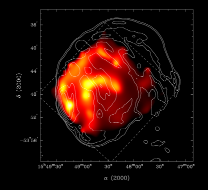
Figure 1.— Broadband (0.3–7 keV) diffuse X-ray image (on a square root scale between $64$ and $480$ photons$\,{\rm cm}^{-2}\,{\rm s}^{-1}\,\mbox{sr}^{-1}$) overlaid with MOST 843 MHz radio contours (at square root scale levels 0.01, 0.02, 0.05, 0.10, 0.17, 0.25, and 0.36 ${\rm~{}Jy~{}beam^{-1}}$; from Whiteoak & Green 1996). The X-ray image is exposure-corrected and was adaptively smoothed to achieve a S/N of 4 (using the CIAO program csmooth). The dashed box denotes the field of view of ACIS-I.

2.1. Source Identification and Optical Counterparts

A major goal of this observation was to search for an internal compact object. There is obviously no bright Crab-like pulsar or pulsar wind nebula (PWN) within Kes 27. However, less energetic PSR/PWN examples have been observed in many other remnants, for example, IC 443 (1.5 kpc distant) and the Vela SNR (0.25 kpc distant) (Olbert et al. 2001; Helfand et al. 2001). Upper limits can be set for these types of PWNe.

If moved to the more distant Kes 27, the IC 443 PWN ($L_{x}=3\times 10^{33}$ ergs s^-1, $2^{\prime}\times 1^{\prime}$ in extent) would appear as a $0.7^{\prime}\times 0.35^{\prime}$ patch in the 2–8 keV X-ray band, with strength $\approx 20$ counts ks^-1. We can set an upper limit of 1 count ks^-1 for an object of this size in the interior of Kes 27, so $L_{x}\leq 1.5\times 10^{32}$ ergs s^-1. Similar reasoning for the Vela PWN ($1.6^{\prime}$ in diameter, $L_{x}=7\times 10^{32}\,{\rm ergs}\,{\rm s}^{-1}$) predicts 7 counts ks^-1 from a $6^{\prime\prime}$ region. In this case we can set an upper limit of 0.5 counts ks^-1, corresponding to $L_{x}\leq 0.5\times 10^{32}$ ergs s^-1. Note that an upper limit depends strongly on the size of the object. Leahy (2004) has suggested that the PSR/PWN within the IC 443 boundary is really associated with the nearer remnant G189.6+3.3. Although this would reduce its luminosity to about one-quarter of that quoted above, our upper limit does not change.

The thermal composite remnant Kes 79 (7 kpc distant) contains an unresolved central compact object (CCO) with $L_{x}=7\times 10^{33}$ ergs s^-1 (Seward et al. 2003). The spectrum is soft, but since absorption is comparable in the two remnants, if this object were in Kes 27, we would expect 40 counts ks^-1, twice as bright as the brightest observed unresolved source. The hardness ratio (defined in the notes to Table 1) should be $\approx 0.5$, and no variation or optical counterpart is expected. As described below, we searched for such an object and did not find one. An upper limit of 0.8 counts ks^-1 yields $L_{x}\leq 1.4\times 10^{32}$ ergs s^-1 for any CCO in Kes 27.

Table 1Chandra Source List

Source	CXOU Name	Count rate $({\rm~{}cts~{}ks}^{-1})$	HR	$J$	$H$	$K$	$B$	$R$	$I$	Comments
(1)	(2)	(3)	(4)	(5)	(6)	(7)	(8)	(9)	(10)	(11)
1	J154722.45–534552.6	0.81$\pm$0.18	0.80$\pm$0.18	14.07	13.54	13.45	17.42	16.05	15.27	?
2	J154737.93–534639.6	2.55$\pm$0.29	-0.10$\pm$0.12	$\cdots$	$\cdots$	$\cdots$	$\cdots$	$\cdots$	$\cdots$	star?, varies
3	J154802.08–534549.3	1.53$\pm$0.23	-0.19$\pm$0.16	12.16	11.44	11.17	16.75	14.77	14.02	star
4	J154805.52–534050.5	0.75$\pm$0.17	-0.64$\pm$0.21	11.50	11.23	11.17	$\cdots$	$\cdots$	$\cdots$	star
5	J154805.67–534018.7	0.67$\pm$0.16	-0.44$\pm$0.25	13.23	12.77	12.71	16.01	14.63	14.28	star
6	J154808.11–534128.1	1.07$\pm$0.20	-0.70$\pm$0.16	10.84	10.67	10.61	11.69	11.59	11.56	star
7	J154816.79–534125.5	7.03$\pm$0.46	0.95$\pm$0.03	$\cdots$	$\cdots$	$\cdots$	$\cdots$	$\cdots$	$\cdots$	AGN
8	J154817.90–535654.4	0.86$\pm$0.18	-0.44$\pm$0.21	13.30	11.66	10.81	15.58	14.26	13.99	star
9	J154819.85–534618.3	2.17$\pm$0.27	0.28$\pm$0.13	10.83	9.74	9.31	19.49	15.63	13.95	star
10	J154820.19–535447.9	1.05$\pm$0.20	-0.54$\pm$0.18	14.86	14.11	13.95	18.08	16.43	15.37	star
11	J154820.78–534222.4	1.07$\pm$0.20	0.15$\pm$0.20	14.01	13.04	12.65	20.61	18.54	17.11	star
12	J154822.10–535548.0	0.83$\pm$0.18	-0.29$\pm$0.22	12.88	12.34	12.21	16.02	14.64	14.05	star
13	J154826.38–534940.0	2.63$\pm$0.29	-0.37$\pm$0.11	13.42	12.70	12.47	17.56	14.87	14.28	star
14	J154829.60–534627.1	3.57$\pm$0.34	-0.53$\pm$0.09	13.24	12.66	12.44	$\cdots$	$\cdots$	$\cdots$	star, flare x10
15	J154832.21–533736.3	1.80$\pm$0.25	0.64$\pm$0.12	$\cdots$	$\cdots$	$\cdots$	$\cdots$	$\cdots$	$\cdots$	AGN?
16	J154832.24–534028.0	0.97$\pm$0.19	0.89$\pm$0.14	$\cdots$	$\cdots$	$\cdots$	$\cdots$	$\cdots$	$\cdots$	AGN?
17	J154832.37–533916.8	57.55$\pm$1.27	-0.55$\pm$0.02	10.24	9.86	9.75	12.20	11.28	10.90	star, varies x2
18	J154832.96–535249.7	0.78$\pm$0.17	-0.52$\pm$0.22	$\cdots$	$\cdots$	$\cdots$	20.02	18.70	16.68	star, varies x3
19	J154837.83–534955.7	2.47$\pm$0.29	-0.52$\pm$0.11	10.59	9.93	9.67	14.18	12.77	11.36	star
20	J154839.05–534316.1	0.72$\pm$0.17	-0.19$\pm$0.25	10.77	9.99	9.66	17.01	14.36	12.92	star
21	J154839.32–534527.1	0.97$\pm$0.19	-0.28$\pm$0.20	11.57	11.30	11.20	13.43	12.41	11.09	star
22	J154840.21–534043.6	13.20$\pm$0.62	-0.71$\pm$0.0	11.50	10.87	10.64	$\cdots$	$\cdots$	$\cdots$	star, varies x3
23	J154840.68–534635.9	0.67$\pm$0.16	-0.44$\pm$0.25	12.52	12.16	12.08	14.57	14.06	13.69	star
24	J154841.14–534005.2	0.78$\pm$0.17	-0.03$\pm$0.24	13.74	13.22	13.01	17.27	15.55	14.91	star
25	J154842.55–535610.1	0.83$\pm$0.18	0.81$\pm$0.18	16.14	15.13	14.56	$\cdots$	$\cdots$	$\cdots$	?
26	J154842.77–535213.4	0.83$\pm$0.18	-0.36$\pm$0.22	13.71	13.27	13.16	16.88	15.32	14.96	star
27	J154853.11–534806.2	1.50$\pm$0.23	-0.43$\pm$0.15	13.76	13.37	13.30	16.79	15.31	14.82	star
28	J154915.48–534407.8	1.34$\pm$0.22	0.72$\pm$0.14	15.91	14.97	14.34	$\cdots$	$\cdots$	$\cdots$	?
29	J154916.18–534244.9	1.34$\pm$0.22	0.80$\pm$0.13	$\cdots$	$\cdots$	$\cdots$	$\cdots$	$\cdots$	$\cdots$	AGN?
30	J154932.56–535026.4	0.59$\pm$0.16	0.00$\pm$0.29	11.55	10.80	10.49	16.40	14.86	13.89	star

Note. — Col. (1): Generic source number. Col. (2): Chandra X-Ray Observatory (unregistered) source name, following the Chandra naming convention and the IAU Recommendation for Nomenclature (e.g., http://cdsweb.u-strasbg.fr/iau-spec.html). Col. (3): On-axis source broad-band count rate. Col. (4): The hardness ratio defined as ${\rm HR}=({\cal H}-{\cal S})/({\cal H}+{\cal S})$, where ${\cal S}$ and ${\cal H}$ are the source count rates in the 0.3–1.5 and 1.5–7 keV bands, respectively. This table only lists sources with individual signal-to-noise ratios greater than 4 in the broad band (${\cal S}+{\cal H}$), with an exception made for source 30, which has a S/N of 3.8 but is obviously discernible in the tricolor image (Fig.3). Cols. (5)–(7): $JHK$ magnitudes from the 2MASS catalog (Skrutskie et al. 2006). Cols. (8)–(10): $BRI$ magnitudes from the USNO-B1.0 catalog (Monet et al. 2003).

We first searched for pointlike sources in the broad band (0.3–7.0 keV) with a wavelet source detection algorithm. Thirty sources with a signal-to-noise ratio S/N$\mbox{\hskip 1.99997pt\raisebox{2.15277pt}{$>$}\raisebox{-2.15277pt}{$\sim$}\hskip 1.99997pt}4$ in the field of view (the range of the four ACIS-I chips) are listed in Table 1 and identified in Figure 2. The spectrum of each source is characterized by a hardness ratio. This is useful in identifying red stars and active galactic nuclei (AGNs). The count rates listed were taken from Chandra automatic processing. Optical data were taken from the Two Micron All Sky Survey (2MASS) catalog (Skrutskie et al. 2006; $JHK$) and the USNO-B1.0 catalog (Monet et al. 2003; $BRI$). If no cataloged source was within $1^{\prime\prime}$ of the X-ray position, no optical data are listed. Most Table 1 sources have soft X-ray spectra and optical counterparts with $0.0<J-H<0.8$ and $0.0<H-K<0.4$. These are identified as stars and are probably of spectral type K or M (Tokunaga 2000). The X-ray spectra of these clearly show less absorption than that of Kes 27, so these are certainly foreground objects — as well they should be. Sources 9 and 11, with harder spectra, are probably highly reddened stars. Even though not many photons were collected, the X-ray flux from some sources is quite variable. The approximate variation is listed.

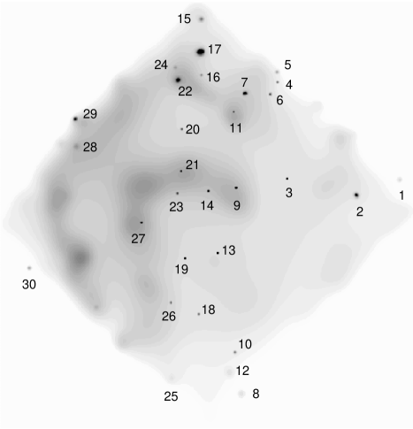
Figure 2.— Identification of the unresolved sources listed in Table 1, showing the adaptively smoothed 0.3–7 keV emission in logarithmic gray scale.

The bright source No.7 is quite hard, is strongly absorbed, and has no counterpart. This is probably a background AGN. Sources 15, 16, and 29 are also hard with no counterparts and are likely to be AGNs. The question marks in Table 1 for these sources indicate classification based on hardness ratio. There were not enough events to determine a spectral shape. A typical AGN with strength of 1 count ks^-1 and with extinction corresponding to at least $2\times 10^{22}\,{\rm cm}^{-2}$, the column density along the path to Kes 27, would have a hardness ratio $\geq 0.7$ with $B\sim 27$, $R\sim 21$, and $H\sim 13$ mag (Seward 2000; NASA/IPAC Extragalactic Database ). There might be a counterpart in the infrared ($JHK$), but not in the optical bands ($BR$). Sources 1, 25, and 28 are hard, with apparent counterparts. Since these three are far from the focal point, the X-ray location is not as accurate as for the more central sources, and there is a higher probability that the counterparts listed are accidental. Sources 25 and 28, with infrared counterparts only, could be AGNs. Sources 2 and 18 are soft, with no 2MASS counterpart. They are classified as stars because they were observed to vary.

The brightest unresolved source, No.17, produced enough counts to derive spectral parameters. The spectrum can best be fitted with a thermal gas plus power law model (see Fig. 3). This source is weakly absorbed [$N_{\scriptscriptstyle\rm H}\sim(6\pm 4)\times 10^{20}\,{\rm cm}^{-2}\,{\rm s}^{-1}$], with power-law photon index $\Gamma\sim 2.9\pm 0.2$, gas temperature $kT\sim 0.77^{+0.07}_{-0.13}\,{\rm keV}$, probably overabundant Ne ([Ne/H]$\sim 3.4^{+3.0}_{-2.3}$), and an unabsorbed 0.5–10 keV flux $F_{x}\sim 5.9\times 10^{-13}\,{\rm ergs}\,{\rm cm}^{-2}\,{\rm s}^{-1}$ ($\chi^{2}=63.3$ with 73 degrees of freedom [dof]). The spectrum of the second brightest unresolved source, No.22, can be fitted with a double thermal gas model [$N_{\scriptscriptstyle\rm H}\sim(6\pm 1)\times 10^{21}\,{\rm cm}^{-2}$, $kT_{1}\sim 0.2^{+0.05}_{-0.02}\,{\rm keV}$, $kT_{2}\sim 1.3^{+1.4}_{-0.6}\,{\rm keV}$, $F_{x}\sim 1.7\times 10^{-12}\,{\rm ergs}\,{\rm cm}^{-2}\,{\rm s}^{-1}$, $\chi^{2}/{\rm dof}=14.3/17$]. These spectra and column densities are quite consistent with the identification as foreground stars.

Figure 3.— Spectrum of the northern hot spot (source 17), fitted with a vmekal+powerlaw model. The source spectrum was extracted from within a 3 $\sigma$ region, and an area of twice the 3 $\sigma$ size surrounding the source region was used as the background. The net count rate is $(5.63\pm 0.12)\times 10^{-2}\,{\rm s}^{-1}$. The spectrum has been adaptively binned to achieve a background-subtracted S/N of 4.

Photons were sparse for most Table 1 sources. A few sources were not easy to classify. Source 2 is soft and has no optical counterpart, but it does not exhibit enough interstellar absorption to be at the distance of the remnant. Source 15 has no counterpart, and the hardness ratio is close to the 0.5 expected from a CCO. Since it is at the limb of the remnant, an AGN identification is more likely.

Two interior sources in the previous ROSAT image, Nos. 2 and 4, were identified as possible PSR/PWN candidates (Seward et al. 1996). These correspond respectively to Chandra sources 14 and 19, which are identified here as foreground stars.

2.2. Spatial Analysis

Figure 1 presents the Chandra image of diffuse emission in the $0.3--7.0\,{\rm keV}$ broad band. Point sources were subtracted, and the pixel values in source regions were replaced with values interpolated from the surrounding area. The X-ray image was then exposure-corrected and adaptively smoothed to achieve a S/N of 4 (using the CIAO program csmooth). Contours of the Molonglo Observatory Synthesis Telescope (MOST) 843 MHz radio emission observation of the remnant (Whiteoak & Green 1996) are superposed on the X-ray image.

To demonstrate the energy dependence of the SNR morphology and the point sources, we also created a tricolor image in three energy bands, as shown in Figure 4: 0.3–1.5 keV (red), 1.5–2.2 keV (green), and 2.2–7.0 keV (blue). These three bands respectively contain the Mg, Si, and S lines, which dominate the remnant’s thermal emission (see §2.3), and have comparable photon fluxes. We first produced exposure maps in the three bands and used these for flat-fielding, accounting for bad-pixel removal, correcting for telescope vignetting, and correcting for variations in quantum efficiency across the detector. The images in the three bands were then smoothed with an adaptive filter (using program csmooth) to achieve a broadband (0.3–7 keV) S/N of 4.

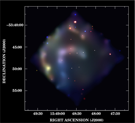
Figure 4.— Tricolor ACIS-I image of Kes 27. The X-ray intensities in the 0.3–1.5, 1.5–2.2, and 2.2–7.0 keV bands are coded red, green, and blue, respectively, and are scaled logarithmically in the ranges 19–170, 19–290, and 27–270 photons$\,{\rm cm}^{-2}\,{\rm s}^{-1}\,\mbox{sr}^{-1}$. The exposure-corrected X-ray maps were adaptively smoothed to achieve a broadband (0.3–7 keV) S/N of 4 (using the CIAO program csmooth).

Figures 1 and 4 show that the X-ray–emitting gas occupies a volume of linear size $\geq 17^{\prime}$ (the size of the ACIS-I CCD chips) and that the centroid of the X-ray emission lies in the eastern half of the remnant. The bright X-ray interior previously seen is now resolved into two semicircular arcs in the northeastern half of the remnant. The emission from the inner arc is harder than that from the outer arc (see Fig. 4). Apart from this bright, hard arc, there is an incomplete, soft arc along the northeastern outskirt. This outer arc is interior to the radio border. The X-ray surface brightness peaks near the southeastern border, where there is a bright X-ray knot (region E1 in Fig. 5) just inside the peak radio emission. This phenomenon is very similar to that seen on the western rim of SNR 3C 391, where the blast wave has been suggested to be propagating into a small, dense region, causing drastic shock deceleration or magnetic field compression and amplification (Chen et al. 2004). The soft, bright, bar-like part of the outer arc in the north appears coincident with a radio arc (Fig. 1). The surface brightness radial profiles are plotted in Figure 6. The two peaks in the northeast profile correspond to the two X-ray arcs, with mean radii of $2.5^{\prime}$ and $6^{\prime}$. The southwest profile shows that the X-ray emission fades with increasing radius, and no shell-like structure can be discerned.

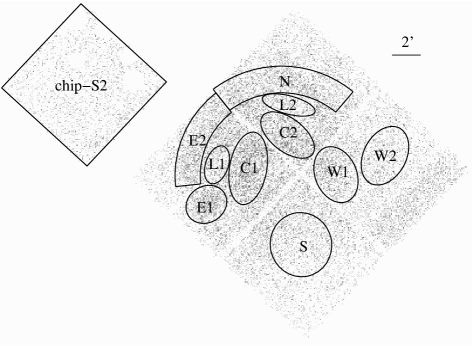
Figure 5.— Raw image of the ACIS observation (with point-like sources removed). The labeled regions are used for spectrum extraction.

Figure 6.— Exposure-corrected radial X-ray (0.3–7 keV) surface profiles for the northeast and southwest parts, centered at R.A.=${15}^{{\rm h}}{48}^{{\rm m}}{37.9}^{{\rm s}}$, decl.=${-53}^{\circ}{48}^{\prime}{01}^{\prime\prime}.9$. The NE part is from position angle $-46.8^{\circ}$ to $133.2^{\circ}$ and the SW part is from $133.2^{\circ}$ to $313.2^{\circ}$. A blank-sky exposure on the ACIS-I chips has been used for background. The dotted lines are plotted according to the White & Long (1991) model, relatively scaled to match the maximum brightness, with parameters $(\tau,C)=(10,50)$ for the left panel and $(\tau,C)=(20,56)$ for the right (see text).

2.3. Spectral Analysis of the Diffuse Emission

After removal of point sources, we extracted the overall spectrum of the diffuse emission from the whole area of the four ACIS-I chips (excluding the peripheral edge) and other on-SNR spectra from 10 substructures marked in the raw-counts image shown in Figure 5. Because the field of view of the four ACIS-I chips is almost entirely covered by the remnant, a local background cannot be obtained from these chips, and hence a double background subtraction method was used. We extracted an off-SNR source-free spectrum from the ACIS-S2 chip (excluding the peripheral edge again; Fig. 5). The respective blank-sky background contributions estimated from the same regions and scaled by the flux at 9.5–12 keV were subtracted from the on- and off-SNR spectra. Individual on-SNR spectra were adaptively binned to achieve a background-subtracted signal-to-noise ratio of 4 and the off-SNR spectrum was binned using a ratio of 3. Each on-SNR spectrum was jointly fitted together with the off-SNR spectrum (Fig. 7). The on-SNR sky background was determined by scaling the off-SNR emission according to the region sizes (Fig. 7, green lines) and is phenomenologically well described by a power law with photon index $\sim 0.7$. Because of the poor signal-to-noise ratio of the off-SNR spectrum below 1.2 keV, the counts below 1.2 keV in all the on-SNR spectra were ignored so as to match the off-SNR one. The XSPEC spectral fitting package (ver. 11.3) was used throughout. For the foreground absorption, the cross sections from Morrison & McCammon (1983) were used, and solar abundances were assumed.

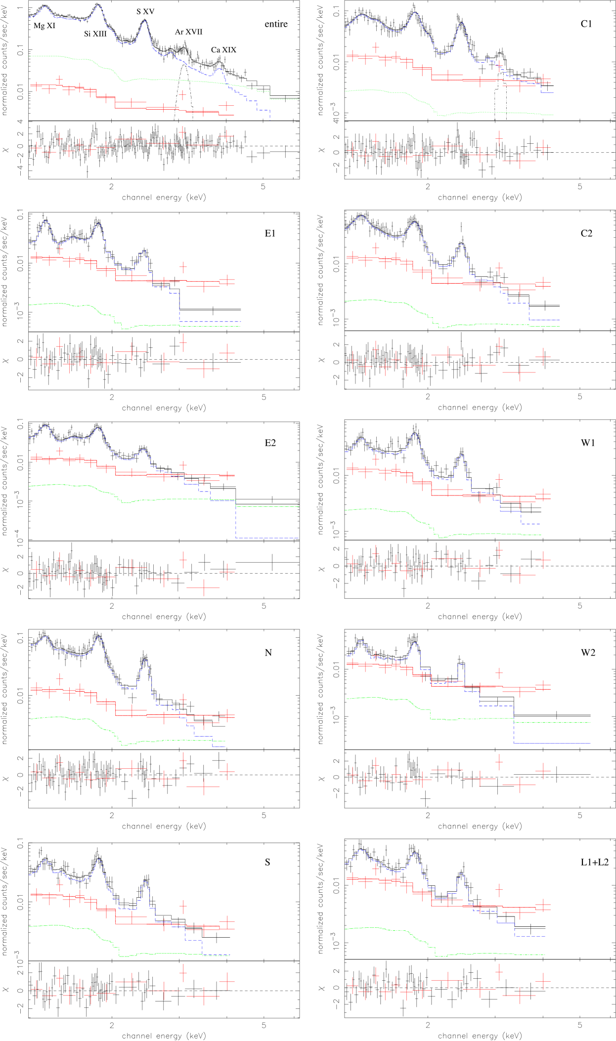
Figure 7.— ACIS spectra of the entire remnant and the small regions shown in Fig. 5. The on-SNR spectra (black solid lines) were rebinned to achieve a background-subtracted S/N of 4, and the off-SNR one (red) was rebinned using a ratio of 3. The net on-SNR spectra (blue) are fitted with an absorbed vpshock model, except for the spectrum of the entire remnant, for which an absorbed vsedov model is used. The sky backgrounds (green) are scaled from the off-SNR spectrum, which is mimicked by a power-law model. The dot-dashed lines around 3.12 keV for the spectral fits of the entire remnant and region C1 are Gaussians accounting for the Ar XVII line.

2.3.1 Overall Spectral Properties

The spectrum of the entire remnant (Fig. 7, top left) shows distinct K$\alpha$ emission line features of metal elements: Mg XI ($\sim 1.34\,{\rm keV}$), Si XIII ($\sim 1.84\,{\rm keV}$), S XV ($\sim 2.43\,{\rm keV}$), Ar XVII ($\sim 3.12\,{\rm keV}$), and Ca XIX ($\sim 3.86\,{\rm keV}$), confirming the thermal origin of the emission. We fitted the net on-SNR spectrum with two absorbed non-equilibrium ionization (NEI) thermal plasma models, vpshock and vsedov (Borkowski et al. 2001; see Table 2). The former model characterizes the plasma parameters of a plane-parallel shock, typified by a constant electron temperature and the shock ionization timescale (the product of the electron density and the time since passage of the shock). The latter is based on Sedov (1959) dynamics, typified by the mean and the electron temperatures immediately behind the shock and by the ionization timescale (the product of the electron density immediately behind the shock and the remnant’s age). Because the NEI models do not include emission from argon, we added a Gaussian at 3.12 keV for the Ar line. Since this spectrum comprises contributions from various regions with different physical properties, it is not expected to be well fitted by a model with a single thermal component. However, it helps to sketch the overall properties of the hot gas interior to the remnant. The two models produce similar physical parameters, but from comparison of the statistical goodness, the vsedov model seems to better fit the spectrum than vpshock. Both models produce elevated abundances of S ($\sim 1.9$–2.8 times solar) and Ca ($\sim$2.8–6.8), indicating that the plasma is metal-enriched. The postblast shock temperature $kT_{s}\sim 0.37$–$0.51\,{\rm keV}$ derived with the vsedov model corresponds to a mean gas temperature $\approx 1.27kT_{s}\sim 0.47$–$0.65\,{\rm keV}$ for the Sedov (1959) case, comparable to the mean temperature $\sim 0.62$–$0.66\,{\rm keV}$ derived with the vpshock model. The mean ionization timescale is $\mbox{\hskip 1.99997pt\raisebox{2.15277pt}{$<$}\raisebox{-2.15277pt}{$\sim$}\hskip 1.99997pt}10^{12}\,{\rm cm}^{-3}\,\mbox{s}$, which indicates that the remnant as a whole is close to, but has not completely reached, ionization equilibrium. The unabsorbed fluxes (0.5–$10\,{\rm keV}$) in the field of view inferred from the two models are (2.3–$2.7)\times 10^{-10}$ and (5.4–$8.6)\times 10^{-10}\,{\rm ergs}\,{\rm cm}^{-2}\,{\rm s}^{-1}$, corresponding to X-ray luminosities of (5.1–$6.0)\times 10^{35}d_{4.3}^{2}$ and (1.2–$1.9)\times 10^{36}d_{4.3}^{2}\,{\rm ergs}\,{\rm s}^{-1}$, respectively.

Table 2Spectral Fitting Results for the Entire Remnant and Estimates of the Das Density

Parameters	vpshock	vsedov
$\chi_{\nu}^{2}$ (dof)	1.89 (162)	1.57 (161)
$N_{\scriptscriptstyle\rm H}$ ($10^{22}\,{\rm cm}^{-2}$)	$2.3\pm 0.1$	$2.3\pm 0.1$
Temperature ($\,{\rm keV}$)	$kT_{x}=0.63^{+0.03}_{-0.01}$${}^{\,\,\rm a}$	$kT_{s}=0.41^{+0.10}_{-0.04}$${}^{\,\,\rm b}$
		$kT_{e}=0.41^{+0.04}_{-0.03}$${}^{\,\,\rm b}$
Ion. Timescale ($10^{11}\,{\rm cm}^{-3}\,{\rm s}$)c	$12.0^{+2.7}_{-4.8}$	$4.19^{+1.15}_{-0.83}$
$fn_{e}n_{\scriptscriptstyle\rm H}V/d_{4.3}^{2}$ ($10^{58}\,{\rm cm}^{-3}$)d	$2.01^{+0.10}_{-0.19}$	$3.36^{+0.85}_{-0.72}$
[Mg/H]	$0.85^{+0.09}_{-0.08}$	$0.63^{+0.08}_{-0.07}$
[Si/H]	$1.00^{+0.07}_{-0.06}$	$1.13^{+0.12}_{-0.09}$
[S/H]	$2.10^{+0.20}_{-0.22}$	$2.47^{+0.36}_{-0.28}$
[Ca/H]	$4.87^{+1.92}_{-1.77}$	$4.45^{+1.84}_{-1.66}$
Flux ($10^{-10}\,{\rm ergs}\,{\rm cm}^{-2}\,{\rm s}^{-1}$)	$2.56^{+0.12}_{-0.25}$	$6.88^{+1.74}_{-1.47}$
$n_{\scriptscriptstyle\rm H}/f^{-1/2}d_{4.3}^{-1/2}$ ($\,{\rm cm}^{-3}$) e	$0.34^{+0.01}_{-0.02}$	$0.44^{+0.06}_{-0.05}$

Note. — The unabsorbed fluxes are in the 0.5–$10\,{\rm keV}$ band. The net count rates of the on- and off-source spectra are $(8.52\pm 0.06)\times 10^{-1}$ and $(1.86\pm 0.14)\times 10^{-2}$ cts$\,{\rm s}^{-1}$, respectively. Confidence ranges are at the 90% level.

The spatial distribution of the relative strength of the S He$\alpha$ emission is shown in the equivalent width (EW) image of this line in Figure 8. This image was constructed using a method similar to those of Hwang et al. (2000) and Park et al. (2002). A major difference of our method from theirs is that we rebin the data using an adaptive mesh, with each bin in each narrow-band image including at least 10 counts (see Warren et al. 2003 for similar binning). The image shows that the S line emission is distributed over a broad region but is strongest in the bright eastern portion of the inner arc. The Ca line is very weak, and we did not produce a Ca EW image.

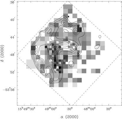
Figure 8.— Equivalent width image of the S He$\alpha$ ($\sim 2.46\,{\rm keV}$) line on a square root scale overlaid with the broadband (0.3–7 keV) diffuse X-ray contours (at seven logarithmic scale levels between 120 and 400 photons$\,{\rm cm}^{-2}\,{\rm s}^{-1}\,\mbox{sr}^{-1}$). The energy range used to extract the S line image is 2.28–2.70 keV, while the low- and high-energy ranges around the S line used to estimate the underlying continuum are 2.07–2.28 and 3.30–3.70 keV. The dashed box denotes the field of view of ACIS-I.

2.3.2 Small-Scale Properties

The spectra of the 10 substructures all show distinct emission lines, indicating optically thin thermal plasma. They were fitted with the vpshock model, and the spectral fit parameters are summarized in Table 3. A Gaussian at $\sim 3.1\,{\rm keV}$ is added to account for the Ar XVII line in the region C1 spectrum. The model fits allow the abundances of key line-producing elements to vary while leaving other abundances fixed to the solar value. Estimates of the hydrogen number densities ($n_{\scriptscriptstyle\rm H}$) inferred from the volume emission measures ($fn_{e}n_{\scriptscriptstyle\rm H}V$, where $f$ is the filling factor of the hot gas and $n_{e}\sim 1.2n_{\scriptscriptstyle\rm H}$ is assumed) are also given in Table 3 (and Table 2 for the entire remnant). In the derivation of the densities we have assumed that the three-dimentional shapes of the elliptical regions (E1, C1, C2, W1, W2, S, L1, and L2) are ellipsoids, those of the arclike regions (E2 and N) are projections of spherical segments, and that of the entire X-ray–emitting volume is a sphere of diameter $17^{\prime}$. Deviations from these assumptions and the nonuniformity of the X-ray–emitting plasma are consolidated into the factors $f$ of the individual regions. The regions show significant spectral variation. The gas temperatures ($\sim 1\,{\rm keV}$) along the inner semicircular arc (regions C1 and C2) are higher than those ($\sim 0.4$–$0.7\,{\rm keV}$) along the softer outer X-ray arc (regions E1, E2, and N). The densest gas in the eastern region E1 is consistent with the suggestion, based on the radio and X-ray brightness peaks, that the forward shock encounters a small dense region there (§ 2.2). The gas density of the low surface brightness regions (L1 and L2) between the two arcs is lower than that in the two bright arcs. The ionization timescales for the small-scale regions (except E1 and E2) are around $10^{12}\,{\rm cm}^{-3}\mbox{s}$ or even higher, and so they may be close to ionization equilibrium, but the ionization timescales for regions E1 and E2 (along the eastern outer shell) are relatively low [(0.6–$3.0)\times 10^{11}\,{\rm cm}^{-3}\mbox{s}$], indicating that the plasma is far from ionization equilibrium. The sulfur abundance in most of the small-scale regions aside from E2 is somewhat higher than solar and seems to peak in region C1, the eastern portion of the inner arc, as shown in the S He$\alpha$ line distribution in the EW map.

Table 3vpshock Fitting Results and Estimates of the Gas Density

Regions	Net Count Rate	$\chi^{2}_{\nu}$ (d.o.f.)	$N_{\scriptscriptstyle\rm H}$	$kT_{x}$	$n_{e}t$	$fn_{e}n_{\scriptscriptstyle\rm H}V/d_{4.3}^{2}$ a	[Mg/H]	[Si/H]	[S/H]	$n_{\scriptscriptstyle\rm H}/f^{-1/2}d_{4.3}^{-1/2}$ b
	($10^{-2}$ cts$\,{\rm s}^{-1}$)		($10^{22}\,{\rm cm}^{-2}$)	(keV)	($10^{11}\,{\rm cm}^{-3}\,{\rm s}$)	($10^{56}\,{\rm cm}^{-3}$)				(cm-3)
E1	$4.00\pm 0.11$	1.07 (54)	$2.7\pm 0.2$	$0.47\pm 0.04$	$1.68^{+1.36}_{-0.42}$	$36.2^{+14.3}_{-11.1}$	$0.74^{+0.28}_{-0.20}$	$0.86^{+0.25}_{-0.19}$	$1.86^{+0.82}_{-0.63}$	$2.1^{+0.4}_{-0.3}$
E2	$6.05\pm 0.14$	0.92 (69)	$2.5^{+0.1}_{-0.2}$	$0.60^{+0.07}_{-0.06}$	$0.89^{+0.76}_{-0.34}$	$29.1^{+10.2}_{-4.6}$	$0.68^{+0.22}_{-0.17}$	$0.74^{+0.21}_{-0.08}$	$1.29^{+0.52}_{-0.45}$	$0.73^{+0.13}_{-0.06}$
N	$7.58\pm 0.15$	1.02 (75)	$1.9\pm 0.2$	$0.60^{+0.04}_{-0.02}$	18.9 ($>5.6$)	$16.7^{+3.4}_{-4.2}$	$0.67^{+0.14}_{-0.21}$	$1.06^{+0.27}_{-0.22}$	$2.48^{+0.94}_{-0.66}$	$0.43^{+0.04}_{-0.05}$
S	$4.18\pm 0.12$	0.98 (54)	$2.3\pm 0.2$	$0.72^{+0.07}_{-0.05}$	12.7 ($>3.8$)	$7.2^{+1.9}_{-1.0}$	$1^{\rm c}$	$1^{\rm c}$	$1.73^{+0.73}_{-0.55}$	$0.25^{+0.03}_{-0.02}$
C1	$8.19\pm 0.16$	1.26 (90)	$1.8\pm 0.6$	$1.21^{+0.45}_{-0.39}$	$3.7^{+22.6}_{-1.6}$	$4.7^{+6.2}_{-1.3}$	$0.83^{+0.52}_{-0.38}$	$1.44^{+0.43}_{-0.32}$	$2.97^{+0.39}_{-0.55}$	$0.43^{+0.28}_{-0.06}$
C2	$5.13\pm 0.13$	0.85 (68)	$2.1^{+0.2}_{-0.3}$	$0.76^{+0.25}_{-0.09}$	$7.2^{+31.8}_{-5.0}$	$6.7^{+2.4}_{-2.0}$	$1.22^{+0.69}_{-0.45}$	$1.10^{+0.40}_{-0.28}$	$1.92^{+0.88}_{-0.59}$	$0.63^{+0.11}_{-0.09}$
W1	$4.12\pm 0.11$	1.00 (54)	$2.6^{+0.3}_{-0.2}$	$0.69^{+0.05}_{-0.04}$	$7.6^{+72.2}_{-5.2}$	$9.8\pm 2.7$	$0.84^{+0.47}_{-0.40}$	$1.05^{+0.38}_{-0.29}$	$1.79^{+0.78}_{-0.56}$	$0.37\pm 0.05$
W2	$2.73\pm 0.10$	1.15 (39)	$2.3^{+0.3}_{-0.4}$	$0.62^{+0.05}_{-0.07}$	7.3 ($>2.0$)	$6.7^{+3.8}_{-2.0}$	$1^{\rm c}$	$1^{\rm c}$	$1.92^{+1.15}_{-0.81}$	$0.30^{+0.09}_{-0.04}$
L1+L2	$3.21\pm 0.10$	1.17 (47)	$2.2^{+0.2}_{-0.3}$	$0.89\pm 0.06$	$5.2^{+13.6}_{-2.8}$	$3.9\pm 1.3$	$1^{\rm c}$	$1^{\rm c}$	$1.60^{+0.60}_{-0.54}$	$0.26\pm 0.04$

Note. — The net count rates of the on-source spectra are listed in the second column; that of the off-source spectrum is $(1.86\pm 0.14)\times 10^{-2}$ cts$\,{\rm s}^{-1}$. Confidence ranges are at the 90% level.

3. Discussion

Kes 27 has been classified as a thermal composite (or mixed-morphology) remnant. It is unusual in that the diffuse thermal X-ray emission peaks not in the center, but along two concentric semicircular arcs. The centroid of the X-ray emission lies in the eastern half of the remnant, and the emission of the inner arc is harder than that of the outer region.

The thermal properties of Kes 27, as inferred from § 2.3, suggest that the X-ray–emitting gas is essentially close to equilibrium of ionization (except along the eastern rim) and enriched with sulfur and calcium. If we adopt $n_{\scriptscriptstyle\rm H}\sim 0.4f^{-1/2}d_{4.3}^{-1/2}\,{\rm cm}^{-3}$ as the mean gas density, then the mass of hot gas is $M=1.4n_{\scriptscriptstyle\rm H}m_{\scriptscriptstyle\rm H}fV\sim 110f^{1/2}d_{4.3}^{5/2}D_{20}^{3}M_{\odot}$, where $m_{\scriptscriptstyle\rm H}$ is the hydrogen atomic mass and $D_{20}$ is the remnant’s diameter $D$ scaled by the radio size, $\sim 20^{\prime}$ (thus $D\approx 25D_{20}d_{4.3}\,{\rm pc}$). The thermal energy contained in the remnant is $E_{th}=(3/2)2.3n_{\scriptscriptstyle\rm H}kTfV\sim 3\times 10^{50}f^{1/2}d_{4.3}^{5/2}D_{20}^{3}\,{\rm ergs}$, where a mean temperature $kT\sim 0.6\,{\rm keV}$ for the hot gas is used. With a shock temperature $kT_{s}\sim 0.4\,{\rm keV}$, the shock velocity would be $v_{s}=(16kT_{s}/3\bar{\mu}m_{\scriptscriptstyle\rm H})^{1/2}\sim 580\,{\rm km}\,{\rm s}^{-1}$, where the mean atomic weight $\bar{\mu}=0.61$. The dynamical age of the remnant, $\sim D/5v_{s}\sim 8.4\times 10^{3}d_{4.3}D_{20}\,{\rm yr}$, is derived with the Sedov (1959) solution, which, because of the unusual morphology and complicated gas components, is only an approximation. The age estimate ($\sim 3.5\times 10^{3}\,{\rm yr}$) based on the ROSAT X-ray observation used a gas temperature ($3.2\,{\rm keV}$) that was too high (Seward et al. 1996). The Sedov model fit yields an ionization timescale $\tau_{\rm Sedov}\sim 4.2\times 10^{11}\,{\rm cm}^{-3}\,\mbox{s}$, which implies a dynamical age $t\approx\tau_{\rm Sedov}/(1.2\times 4n_{\scriptscriptstyle\rm H})\sim 7\times 10^{3}f^{1/2}d_{4.3}^{1/2}\,{\rm yr}$ (where we have assumed that the preshock density is similar to the mean interior density $n_{\scriptscriptstyle\rm H}$). This is similar to the above Sedov age. On the other hand, the upper limit on the mean ionization timescale derived with the vpshock model (Table 2) gives an age $\sim 9\times 10^{4}f^{1/2}d_{4.3}^{1/2}\,{\rm yr}$. This is similar to the ionization age ($>8\times 10^{4}\,{\rm yr}$) found in the ASCA X-ray study (Enoguchi et al. 2002) and is comparable to the remnant’s radiative cooling timescale, $t_{\rm cool}\sim 4\times 10^{4}E_{51}^{0.24}[n_{0}/(0.4\,{\rm cm}^{-3})]^{-0.52}\,{\rm yr}$, where $E_{51}$ is the SNR’s explosion energy in units of $10^{51}\,{\rm ergs}$ and $n_{0}$ is the preshock density (Falle 1981). In this case the postshock temperature would be $\mbox{\hskip 1.99997pt\raisebox{2.15277pt}{$<$}\raisebox{-2.15277pt}{$\sim$}\hskip 1.99997pt}1\times 10^{6}\,{\rm K}$ and thus the gas would be X-ray–faint. This does not agree with the postshock temperatures derived from the spectral fits and the fact that the eastern rim of the SNR is X-ray–bright. A possibility to reconcile the different estimates might be for the X-ray emitting gas to have a very low filling factor, $f\mbox{\hskip 1.99997pt\raisebox{2.15277pt}{$<$}\raisebox{-2.15277pt}{$\sim$}\hskip 1.99997pt}1\times 10^{-2}D_{20}^{2}d_{4.3}$, but this seems unlikely.

The mass of the X-ray–emitting gas, $\sim 10^{2}f^{1/2}M_{\odot}$, suggests that the SNR is not in the free-expansion phase and is probably dominated by the swept-up ambient medium. Even so, Kes 27 appears to be enriched in S and Ca, and this is not a unique case. One sample of 23 thermal composite (or mixed-morphology) SNRs showed that 10 of them to be detected as metal-enhanced (Lazendic & Slane 2006). The contribution of supernova ejecta has been suggested to be the cause of both the elevated metal abundances and the X-ray brightening in the central regions. For example, the overabundant Mg, Si, and (possibly) S in thermal composite SNR G290.1$-$0.8 (Slane et al. 2002) and the Ne, Si, and S enhancement in W44 are ascribed to supernova ejecta (Shelton et al. 2004).

Environments of nonuniform density are often seen around SNRs, especially those adjacent to dense clouds. This sometimes is consistent with systematic variation of the intervening hydrogen column density along the line of sight to the SNR, as for 3C 391 (Chen et al. 2004) and 3C 397 (Safi-Harb et al. 2005). Kes 27’s HI density enhancement is found to the east of the remnant (McClure-Griffiths et al. 2001), and the Spitzer IRAC 8 $\mu$m observation (Reach et al. 2006) shows a large-scale environment with a density gradient increasing from west to east. However, our X-ray study of Kes 27 does not show a clear trend of $N_{\scriptscriptstyle\rm H}$ (and spectral) variations along the density gradient (although E1 is the only region showing a significantly higher value; Table 3). This may indicate that the environmental hydrogen column density may take only a very low fraction in the intervening interstellar column ($\sim 2\times 10^{22}\,{\rm cm}^{-2}$), either because the cloud complex in the vicinity is not very compact or bacause it is not very large.

The double X-ray rings are not expected in either the cloud evaporation or the thermal conduction model. In the latter (Cox et al. 1999; Shelton et al. 1999), thermal conduction in the remnant smooths out the temperature gradient from the hot interior to the cooler shell and increases the central density, resulting in luminous X-rays in the interior; this effect is dominant in the radiative stage. This model predicts a centrally peaked X-ray surface brightness for the SNR and, usually, a high ionization timescale for the hot gas, inconsistent with our observation. The cloud evaporation model (White & Long 1991) suggests that when an SNR expands in an inhomogeneous interstellar medium whose mass is mostly contained in small clouds, the clouds engulfed by the blast wave can be evaporated to slowly increase the density of the interior hot gas; as a result, the SNR appears internally X-ray–brightened. This model can reproduce an X-ray–bright inner ring like that in the northeastern half of Kes 27 and can also reproduce a fading-out radial surface brightness profile like that in the southwestern half (see Fig.‘6). A representative fit to the inner ring’s brightness profile using the cloud evaporation model requires the ratio of the cloud evaporation timescale to the SNR’s age to be $\tau=10$ and the ratio of the mass of the cloudlets to the mass of the intercloud medium to be $C=50$. The fit is not unique, and combinations of $\tau=8$–12 and $C=40$–60 produce similar profiles (relatively scaled to match the maximum brightness). A representative fit to the southwest radial brightness profile would need $\tau=20$ (15–25) and $C=56$ (45–70). However, the generally higher inner gas temperature as compared with the outer region is not expected for such high $\tau$- and $C$-values in the evaporation model. Moreover, this model overestimates the surface brightness inside the inner ring and cannot reproduce the outer X-ray ring in the northeast. It also cannot naturally explain why the physical conditions exemplified by the parameters $\tau$ and $C$ should be different in the two halves and why there are not two rings in the southwestern half, in contrast to the northeastern.

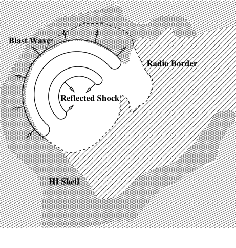
Figure 9.— Diagram showing the structure and environment of the Kes 27 remnant.

Another scenario is required to account for the unusual X-ray morphology of Kes 27, which is different from that of other thermal composite remnants. Actually, the explanation must be consistent with the following facts: (1) The large-scale environment around Kes 27 has a density gradient increasing from west to east, as revealed in the infrared (Reach et al. 2006). (2) As sketched in Figure 9, the remnant is surrounded by a “crocodile’s mouth”–like H I shell (McClure-Griffiths et al. 2001). (3) In X-rays, the remnant is brightened in the northeastern half and fades out to the southwestern low-density region. (4) The inner and outer X-ray arcs are both located in the northeastern half, where the ambient medium is denser than in the southwest. (5) The outer arc is in contact with the H I shell. (6) The inner arc is hotter than the outer arc. (7) As noted by Enoguchi et al. (2002), the radio polarization observed by Milne et al. (1989) is strong in both the eastern rim and the center.

We suggest that both the outer and inner arcs represent shock waves, propagating outward and inward, respectively. The observed polarization in the eastern rim and the center is due to shocked and compressed matter in the two arcs. The present inward shock is not the initial reverse shock caused by expansion into low-density circumstellar material. The remnant is middle-aged, and this has long passed (McKee 1974). The present inward shock is a reverse shock due to the distant HI shell.

A comprehensive scenario is as follows: The massive progenitor exploded in a cavity excavated by the strong stellar wind and ionizing radiation. Because of the density gradient in the environmental medium, the wind cavity had a small radius in the east and a large radius in the west, or may even not have been confined in the west. After the supernova explosion, in the west and southwest, the blast wave propagated into a low-density medium, and the X-ray emission is faint. In the north and east, the blast wave has hit the cavity wall. A transmitted shock is now propagating into the dense wall, and a reflected shock is traveling back toward the remnant’s center, shocking the supernova ejecta to higher temperature. The outer arc contains gas heated by the transmitted shock, and the inner arc is the interior metal-enriched gas heated by the reflected shock (see again Fig. 9). Shock-heated S atoms in the compressed inner arc emit a strong He$\alpha$ line.

Chen et al. (2003) considered a thin-shell model for a blast shock hitting a wind-cavity wall but did not include shock reflections. Dwarkadas (2005, 2007) simulated shocks reflected back from a cavity wall, and a picture of shock reflection and transmission similar to what is seen in Kes 27 was predicted. To capture the essential physics essence, we use the theory of reflected shocks described by Sgro (1975) to estimate some relevant parameters. For a shock reflected by a dense wall, the temperature ratio between the post–reflected-shock gas and post–transmitted-shock gas is given by

$$\frac{T_{r}}{T_{t}}=\frac{A}{A_{r}},$$ (1)

where $A_{r}$ is the density contrast between the post–reflected-shock gas and post–incident-shock gas and $A$ is the wall-to-cavity density contrast, which is related to $A_{r}$ as

$$A=\frac{3A_{r}(4A_{r}-1)}{\{[3A_{r}(4-A_{r})]^{1/2}-\sqrt{5}(A_{r}-1)\}^{2}}.$$ (2)

The pressure ratio of the post–transmitted-shock gas to the post–incident-shock gas is

$$\beta=\frac{4A_{r}-1}{4-A_{r}}.$$ (3)

Using these equations, we plot the functional relations of $T_{r}/T_{t}$, $A_{r}$, and $\beta$ with $A$ in Figure 10. Regions E2 versus C1 and N versus C2 represent two pairs of transmitted versus reflected shocks. The ranges of the temperature ratios obtained from Table 3 are shown in Figure 10. Because there is a large scatter in the fitted temperatures, there are large uncertainties in the wall-to-cavity density $A$, which seems to be $\sim$ 2. The density contrast between the post–reflected-shock gas and postincident shock gas $A_{r}$ is around 1.3. If regions W1, W2, and S can be taken as roughly indicative of a post–incident-shock gas density $\sim(0.2-0.4)f^{1/2}d_{4.3}^{1/2}\,{\rm cm}^{-3}$ (Table 3), then the post–reflected shock density $0.4-0.6f^{1/2}d_{4.3}^{1/2}\,{\rm cm}^{-3}$ in C1 and C2 is consistent with the values of $A_{r}$ (although this estimate is crude, because the filling factor $f$ may vary from region to region).

Figure 10.— Parameters for the reflected shock. The large box represents the value ranges for region pair E2 and C1, and the small box is for region pair N and C2 (see text).

Such a reflected shock launched from the cavity wall is consistent with the observed properties of Kes 27. As the remnant continues to age, the transmitted shock in the dense medium will become fainter in X-rays, while the reflected shock will converge in the center, producing a truly centrally X-ray–brightened morphology. The reflection of shocks is thus another mechanism that may produce thermal composite remnants.

4. Summary

We have observed the thermal composite SNR Kes 27 with the ACIS-I detectors on Chandra and performed a spatially resolved spectroscopic study of the remnant. The main results are summarized as follows.

1. We have detected 30 pointlike X-ray sources superposed on the remnant, with S/N$\mbox{\hskip 1.99997pt\raisebox{2.15277pt}{$>$}\raisebox{-2.15277pt}{$\sim$}\hskip 1.99997pt}4$. Most are foreground stars, and some are probably background AGNs. None has the properties expected from a central compact stellar remnant. The upper limit to the luminosity of a CCO or a diffuse PWN is $\sim 1.5\times 10^{32}$ ergs s^-1.

2. The X-ray spectrum of Kes 27 is characterized by K lines from ionized Mg, Si, S, Ar, and Ca. Most of the X-ray–emitting regions are found to be enriched in sulfur. Calcium is also over-abundant in the remnant. The hot gas in the remnant is essentially close to ionization equilibrium (except for that along the eastern rim).

3. Images of the remnant show previously unseen double X-ray arc structures. There is an outer X-ray arc and an inner, harder, concentric arc. These two shell-like features are located in the northeastern half of the remnant, and the X-ray surface brightness fades away with increasing radius to the southwest. The X-ray intensity peak coincides with the radio-bright region along the eastern border. The gas in the inner region is at higher temperature.

4. The overall morphology can be explained by the evolution of the remnant in an ambient medium with a density gradient increasing from west to east. The remnant was probably born in a preexisting cavity created by the progenitor star. The outer shock has hit the cavity wall and is now in the denser wall material, and the inner arc indicates gas heated by a reflected shock. This process may explain the X-ray morphology of this and even other thermal composite supernova remnants.

This work was supported by Chandra grant GO3-4074X. Y. C. acknowledges support from National Natural Science Foundation of China grants 10725312, 10673003, and 10221001. F. D. S. thanks Scott Wolk for useful advice on star identification and Y.C. also thanks Jasmina Lazendic and Pat Slane for previous collaboration on issues regarding reflected shock waves. We also thank an anonymous referee for helpful suggestions.

References

- (1) Borkowski, K. J., Lyerly, W. J., & Reynolds, S. P. 2001, ApJ, 548, 820
- (2) Chen, Y., Su, Y., Slane, P. O., & Wang, Q. D. 2004, ApJ, 616, 885
- (3) Chen, Y., Zhang, F., Williams, R. M., & Wang, Q. D. 2003, ApJ, 595, 227
- (4) Cox, D. P., Shelton, R. L., Maciejewski, W., Smith, R. K., Plewa, T., Pawl, A., & Rózyczka, M. 1999, ApJ, 524, 179
- (5) Dwarkadas, V. V. 2005, ApJ, 630, 892
- (6) Dwarkadas, V. V. 2007, ApJ, 667, 226
- (7) Enoguchi, H., Tsunemi, H., Miyata, E., & Yoshita, K. 2002, PASJ, 54, 229
- (8) Falle, S.A.E.G. 1981, MNRAS, 195, 1011
- (9) Green, A. J., Frail, D. A., Goss, W. M., & Otrupcek, R. 1997, AJ, 114, 2058
- (10) Harrus, I. M., Hughes, J. P., Singh, K. P., Koyama, K., & Asaoka, I. 1997, ApJ, 488, 781
- (11) Helfand, D. J., Gotthelf, E. V. & Halpern, J. P., 2001, ApJ, 556, 380
- (12) Hwang, U., Holt, S. S., & Petre, R. 2000, ApJ, 537, L119
- (13) Kawasaki, M., Ozaki, M., Nagase, F., Inoue, H., & Petre, R. 2005, ApJ, 631, 935
- (14) Kesteven, M. J. & Caswell, J. L. 1987, A&A, 183, 118
- (15) Lazendic, J. S. & Slane, P. O. 2006, ApJ, 647, 350
- (16) Leahy, D. 2004, AJ, 127, 2277 (addendum 128, 1478)
- (17) McClure-Griffiths, N. M., Green, A. J., Dickey, J. M., Gaensler, B. M., Haynes, R. F., & Wieringa, M. H. 2001, ApJ, 551, 394
- (18) McKee, C. F. 1974, ApJ, 188, 335
- (19) Milne, D. K., Caswell, J. L., Kesteven, M. J., Haynes, R. F., & Roger, R. S. 1989, PASAu, 8, 187
- (20) Monet,, D. G., et al. 2003, The USNO-B1.0 catalog (Flagstaff: US Nav. Obs.)
- (21) Morrison, R., & McCammon, D., 1983, ApJ, 270, 119
- (22) Olbert, C. M., Clearfield, C. R., Williams, N. E., Keohane, J. W. & Frail, D. A., 2001, ApJ, 554, L205.
- (23) Park, S., Roming, P. W. A., Hughes, J. P., Slane, P. O., Burrows, D. N., Garmire, G. P., & Nousek, J. A., 2002, ApJ, 564, L39
- (24) Petruk, O. 2001, A&A, 371, 267
- (25) Reach, W. T., Rho, J., Tappe, A., Pannuti, T. G., Brogan, C. L., Churchwell, E. B., Meade, M. R., Babler, B., Indebetouw, R., & Whitney, B. A. 2006, AJ, 131, 1479
- (26) Rho, J.H., & Petre, R. 1998, ApJ, 503, L167
- (27) Safi-Harb, S., Dubner, G., Petre, R., Holt, S. S., & Durouchoux, P. 2005, ApJ, 618, 321
- (28) Sedov, L. I. 1959, Similarity and Dimensional Methods in Mechanics (New York: Academic)
- (29) Seward, F.D., 1990, ApJS, 73, 781
- (30) Seward, F.D., 2000, in Allen’s Astrophysical Quantities, ed. A. N. Cox (4th ed.; New York: AIP), Chapter 9, 202.
- (31) Seward, F. D., Kearns, K. E., & Rhode, K. L. 1996, ApJ, 471, 887
- (32) Seward, F. D., Slane, P. O., Smith, R. K. & Sun, M., 2003, ApJ, 584, 414
- (33) Sgro, A. G. 1975, ApJ, 197, 621
- (34) Shelton, R. L., Cox, D. P., Maciejewski, W., Smith, R. K., Plewa, T., Pawl, A., & Rózyczka, M. 1999, ApJ, 524, 192
- (35) Shelton, R. L., Kuntz, K. D., & Petre, R. 2004, ApJ, 611, 906
- (36) Skrutskie, M. F., et al. 2006, AJ, 131, 1163
- (37) Slane, P., Smith, R. K., Hughes, J. P., Petre, R. 2002, ApJ, 564, 284
- (38) Tokunaga, A.T., 1999, in Allen’s Astrophysical Quantities, ed. A. N. Coxs (4th ed.; New York: AIP), Chapter 7, 151.
- (39) Warren, J. S., Hughes, J. P., & Slane, P. O. 2003, ApJ, 583, 260
- (40) White, R. L., & Long, K. S. 1991, ApJ, 373, 543
- (41) Whiteoak, J. B. Z. & Green, A. J. 1996, A&AS, 118, 329
- (42) Yusef-Zadeh, F., Wardle, M., Rho, J., & Sakano, M. 2003, ApJ, 585, 319