Superfluidity and phase transitions in a resonant Bose gas
Abstract
The atomic Bose gas is studied across a Feshbach resonance, mapping out its phase diagram, and computing its thermodynamics and excitation spectra. It is shown that such a degenerate gas admits two distinct atomic and molecular superfluid phases, with the latter distinguished by the absence of atomic off-diagonal long-range order, gapped atomic excitations, and deconfined atomic -vortices. The properties of the molecular superfluid are explored, and it is shown that across a Feshbach resonance it undergoes a quantum Ising transition to the atomic superfluid, where both atoms and molecules are condensed. In addition to its distinct thermodynamic signatures and deconfined half-vortices, in a trap a molecular superfluid should be identifiable by the absence of an atomic condensate peak and the presence of a molecular one.
pacs:
Valid PACS appear hereI Introduction
I.1 Background
Remarkable experimental advances in manipulating degenerate atomic gases have opened a new era in studies of highly coherent, interacting quantum many-body systems. One of the most striking advances is the ability to finely control atomic two-body interactions by tuning with a magnetic field the energy (detuning) of the molecular Feshbach resonance (FR) through the atomic continuum.F62 ; TTHK99 This technique has led to a realization of a long-sought-after s-wave paired superfluidity in bosonicWFHRH00 ; DCTW02 and fermionic atomic gases.J03 ; GRJ04 ; Z04 For fermionic atoms, it also allowed the system to be tuned between the BCSBCS57 regime of weakly-paired, strongly overlapping Cooper pairs (familiar from solid-state superconductors), and the BEC regime of tightly bound, weakly-interacting Bose-condensed diatomic molecules.
Although this crossover has received considerable attention,MRE93 ; TFMK01 ; OG02 ; MKH02 ; AGR04 ; CSL05 ; GR07 because of the absence of qualitative differences between the BCS and BEC s-wave paired fermionic superfluids, their equilibrium properties are already qualitatively well described by early seminal works.E69 ; L80 ; NS85 In fact for a narrow FR (unfortunately not realized by most current experimental systems), the crossover can even be computed quantitatively, as a perturbation series in the ratio of the FR width to the Fermi energy.AGR04 ; GR07 In such narrow FR systems the crossover to BEC takes place when the FR detuning (quasi-molecule’s rest energy) ranges from twice the Fermi energy (when it first becomes favorable to convert a finite fraction of the Fermi-sea into molecules stabilized by Pauli-blocking) down to zero energy, where all the fermions have become bound into Bose-condensed diatomic molecules. The complementary broad resonance regime of most experiments,GRJ05 particularly near a universal unitary pointH04 has been successfully studied using quantum Monte CarloCR05 ; BDM07 ; BPST06 and field theoretic -expansionSon06 ; NS06 and -expansionNS06 ; VSR06 methods borrowed from critical phenomena.
As was recently pointed outRPW04 ; RDSS04 and is the subject of this paper, the phenomenology of resonantly interacting degenerate bosonic atoms contrasts strongly and qualitatively with this picture.Nozieres For a large positive detuning, molecules are strongly energetically suppressed and unpaired atoms (as in any bosonic system at zero temperature) form an atomic superfluid (ASF), exhibiting atomic off-diagonal long-range order (ODLRO).P51 In the opposite extreme of a large negative detuning, free atoms are strongly disfavored (gapped), pairing up into stable bosonic molecules, that then, at , form a diatomic molecular superfluid characterized by a molecular ODLRO. The MSF does not exhibit atomic ODLRO, nor the associated atomic superfluidity. Together with a gapped atomic excitation spectrum and correlation functions (characteristics that extend to finite temperature), these features qualitatively distinguish it from the ASF.

In a trapped, dilute atomic gas the existence of these two qualitatively distinct superfluid phases should be most directly detectable through independent images of atomic and molecular density profiles. As illustrated in Fig. 1(a), the atomic component should exhibit a BEC peak in the ASF phase, that is absent in the MSF phase, shown in Fig. 1(b). Both superfluid phases are distinguished from the normal state by the BEC peak in the molecular density profile, as illustrated in the insets to these figures.
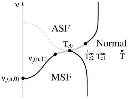
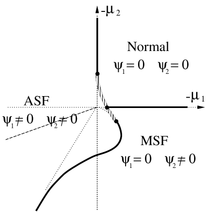
Because of its paired nature, a complementary distinguishing characteristic of a MSF are deconfined (half-) vortices, topological defects that, in contrast, are linearly confined in the ASF state. Consequently, as illustrated in Fig. 2, a thermodynamically sharp quantum phase transition, at an intermediate critical Feshbach resonance detuning , must separate the MSF and ASF phases. Each in turn is also separated by a finite-temperature transition from the “normal” (N) state lacking any order (i.e., breaking no symmetries).
Experimental observations of these and associated predictions have so far been precluded by a short lifetime of the vibrationally hot molecular state.vibration The latter is believed to be limited by 3-body recombination and strongly enhanced atom-molecule scattering near the resonance. In contrast to Fermi systems,J03 ; GRJ04 ; Z04 where Pauli exclusion greatly extends the molecular lifetime for a positive scattering length and stabilizes the Fermi-sea for negative scattering lengths by suppressing multi-body collisions,PSS04 the resonantly interacting bosonic atomic gas is observed to be highly unstable in the negative two-body scattering length regime.D01 ; BM05 Viable proposals for surmounting these problems are currently being investigated. These include use of an adiabatic ramp of the detuning through resonance,G03 or a two-photon Raman transition to transfer the Feshbach molecular states to a lower lying vibrational state.SM04
Although no direct evidence for an equilibrium Bose molecular condensate exists, observed resonant atomic loss in a stimulated Raman transition in 87Rb (Ref. Heinzen00, ) and time domain density oscillations in 85Rb (Ref. DCTW02, ) are consistent with a coherent transfer of population from free bosonic atoms to diatomic molecules.KH02 ; R98 It is not at the moment clear (at least to the present authors) whether current experimental difficulties of stabilizing bosonic atom-molecule mixtures near a FR are fundamental or technical and system specific. One possible fundamental source of instability in bosonic atom systems is the existence of Efimov bound states of bosonic atom triplets.E71 ; GurarieDiscuss At least at a theoretical model level these can be suppressed by a sufficiently strong three-body repulsion. Even in the unfavorable scenario, where such phases of bosons near a FR are indeed metastable (as most states of degenerate atoms ultimately are) one expects that ideas discussed here should be important on sufficiently short time scales and for understanding of the associated nonequilibrium dynamics.
The rest of the paper is organized as follows. The Introduction is concluded with a summary of the main results and their experimental implications. In Section II a microscopic two-channel model, that is believe to accurately describe resonantly-interacting atomic bose gas is introduced. The model is first used to compute the two-body s-wave scattering, showing that it correctly captures the Feshbach resonance phenomenology. Matching the computed scattering amplitude to its measured counterpart allows one to relate parameters appearing in the Hamiltonian to experimental observables. In Section III a general symmetry-based discussion of the expected phases and associated phase transitions in this system is presented. In Section IV, by minimizing the corresponding imaginary-time coherent state action, the generic mean field phase diagram for the system is mapped out. In Sections V and VI, this Landau analysis is supplemented by detailed microscopic calculations of phase boundaries, spectra, condensate depletion and superfluid density for a dilute, weakly-interacting gas. The asymptotic nature of the ASF–MSF phase transition is discussed in Section VII. In Section VIII the mean field and perturbative analyses, performed within a two-channel model, are supplemented with a variational theory of a one-channel model. The latter is a better description of bosons in which the paired state is absent (i.e., there is no long lived metastable paired state with distinct internal quantum numbers) once the two-body attraction becomes too weak to bind atom pairs (which includes, of course, the more familiar regime of two-body repulsion). In Section IX topological defects, vortices and domain walls, in the ASF are studied, and the ASF–MSF and SF-to-normal fluid transitions are characterized in terms of a proliferation of these topological defects. The paper is concluded in Section X.
I.2 Summary of results
In this paper a considerable elaboration and extension of predictions reported in a recent LetterRPW04 are presented. The primary results are summarized by the density profiles in Fig. 1 and the phase diagrams in Figs. 2 and 10, characterizing the phases and phase transitions of a resonant Bose gas. As illustrated there, it is found that Feshbach-resonantly interacting atomic Bose gas, in addition to the normal state exhibits two distinct low-temperature superfluid states. The first, appearing at positive detuning, is the more conventional atomic superfluid, characterized by coexisting atomic and molecular BEC and their associated ODLROs, with finite order parameters and , respectively. The other, more exotic, MSF state, appearing at low temperature and negative detuning, is characterized by superfluidity of diatomic molecules, with a finite molecular condensate order parameter . It is distinguished from the ASF by the absence of atomic ODLRO, i.e., inside the MSF phase .
As illustrated in detail in Sec. IV.2, a finite always implies a finite . In the presence of an atomic condensate, , the Feshbach resonance coupling allows a scattering of two Bose-condensed atoms out of the atomic BEC into the molecular BEC (i.e., ASF is really a superposition of Bose-condensed open-channel atoms and Bose-condensed closed-channel molecules) and therefore acts like an ordering “field” on the molecular order parameter. This implies that a state in which atoms are condensed but molecules are not is forbidden by general symmetry principles.decoupledBEC
As noted above, a vivid signature of two distinct superfluid orders should be detectable via time-of-flight shadow images. In the dilute regime (described by a BEC approximation), the resulting images are schematically illustrated in Fig. 1. At higher densities, where a local density approximation is more appropriate, it is expected that for a range of atom number and detuning, phase boundaries as a function of chemical potential in the bulk system (see e.g., Fig. 10) will translate into shell structureshellsMott1 ; shellsMott2 ; shellsMott3 which should also be observable experimentally in time-of-flight shadow images.
As for any neutral superfluid, ASF and MSF are each characterized by an acoustic (Bogoliubov) “sound” mode, illustrated in Fig. 3, corresponding to long wavelength condensate phase fluctuations, with long wavelength dispersions
| (1) |
where (with ASF or MSF, or equivalently 1 or 2) are the associated sound speeds with given by (149) and given by (166) in terms of the interaction parameters of the model (see Sec. VI.2).
In the ASF state the gapless mode corresponds to in-phase fluctuations of the atomic and molecular condensates. However, as illustrated in Fig. 3, in contrast to ordinary superfluids, ASF and MSF also each exhibit a gapped branch of excitations,
| (2) |
with gaps given explicitly by (151) and (160), while the quadratic corrections may be inferred from the general forms (115) and (138) of the spectra. In the ASF the gap is controlled by out-of-phase fluctuations of the atomic and molecular condensates, and is set by the Feshbach coupling .
In the MSF, gapped excitations are single atom-like quasiparticles akin to Bogoliubov excitations in the paired BCS state, that however do not carry a definite atom number. These single-particle excitations are “squeezed” by the presence of the molecular condensate, offering a mechanism to realize atomic squeezed states.laser_analogy We expect that these gapped, atomic quantum fluctuations associated with the presence of the molecular condensate can be measured by interference experiments, similar to those reported in Ref. Kasevich01, . As detailed below, the low-energy nature of these excitations is guaranteed by the vanishing of the gap at the MSF–ASF transition, , with .

In the dilute weakly interacting limit appropriate to atomic gases, the ASF–N and MSF–N transition temperatures, and , respectively, for a three-dimensional (3d) bulk uniform system are well approximated by
| (3) |
with , , , , and . One sees that , with the asymptotic ratio set by the mass and boson number that both differ by a factor of two between the two phases. When interactions are included, for the asymptotic nature of these thermal transitions is in the well-studied classical 3d XY universality class.
As illustrated in Fig. 2 (see also Figs. 10 and 11), in the vicinity of the critical endpoint , , where the three phases, N, MSF, ASF meet, a coupling of the molecular and atomic superfluid order parameters converts a section (between the tricritical points TC1 and TC2) of the (otherwise) continuous N–ASF and MSF–ASF transitions to first order.BM05 The resulting crossing point at , that terminates a continuous N–MSF transition is a critical endpoint (CEP). In the dilute limit, the CEP temperature is given by
| (4) |
As illustrated in Secs. IV and VII, the appearance of a first order transition (even in mean field theory) near N–MSF continuous boundary, is a generic feature resulting from the coupling of the ASF order parameter to the critical MSF order parameter.RPW04
The corresponding transition temperatures in a trap (here distinguished from bulk quantities by a tilde) are also easily computed and in 3d are given by
| (5) |
with , and . The transition temperatures in the limit of asymptotically large positive () and negative () detuning (), and at the tricritical point (), are given, respectively, by
| (6) | |||||
| (7) |
where is the trap frequency. Comparing the first lines of (3) and (5), note that the latter is now approached linearly with, rather than as the square-root of the reduced detuning from either side.
In the dilute limit the thermodynamics is also easily worked out. In the 3d bulk system, the condensate densities for the atomic and molecular BEC are given, respectively, by
| (8) | |||||
| (9) |
where and is the extended zeta function.GR
As illustrated in Fig. 2 the MSF–ASF transition takes place at a critical value of detuning determined by the strength of atomic and molecular interactions, shifting it away from its noninteracting value of . At zero temperature this is a continuous quantum phase transition that for a -dimensional system is in the -dimensional classical Ising universality classcommentFirstOrder ; FB97 ; LL04 with
| (10) |
where , , and are, respectively, the atom-atom, atom-molecule and molecule-molecule interaction strengths, related in the standard way to the corresponding scattering lengths,GR07 and is the Feshbach resonance coupling. The transition at is characterized, upon approach from the MSF side, by the vanishing of the single-atom excitation gap , and, upon approach from the ASF side, by the disappearance of the atomic condensate . At zero temperature, in the critical region these are predicted to vanish according to
| (11) |
where and are, respectively, the order parameter and correlation length exponents for the -dimensional Ising model. One may hope that when long-lived molecular condensates are produced, nontrivial behavior of and the full excitation spectra, may be observed in Ramsey fringesDCTW02 and in Bragg and RF spectroscopy experiments BraggKetterle ; RFChin ; RFKetterle ; BraggBruunBaym .
At finite temperature, away from the critical endpoint the transition is in the classical -dimensional Ising universality class. Scaling, together with the relevance (in the renormalization group sense) of at the quantum critical point, also implies a universal shape of the low part of the MSF–ASF phase boundary
| (12) |
illustrated in Fig. 2.
The dashed curve, inside the ASF phase of the phase diagram (Figs. 2 and 10) denotes a crossover (that becomes sharp with a vanishing Feshbach resonance coupling ) between ASF regimes with low and high values of the molecular condensate . In the absence of the coupling, the molecules would condense on their own for . For small the weak symmetry breaking field generated by the atomic condensate smears this transition into a ASF-AMSF crossover, and leads to small, but finite, even for .
As for any superfluid, the ASF and MSF phases also exhibit interaction-driven condensate depletion , quantifying the fact that, even at , not all atoms are in the condensate. At these are computed in Sec. VI.4. An interesting feature, illustrated in Fig. 4, is that exhibit a cusp maximum at ,
| (13) |
associated with enhanced role of quantum fluctuations at the MSF–ASF transition. The maximum depletion is given by
| (14) |
where is the molecule-molecule s-wave scattering length. Outside the critical region one expects , crossing over to inside it, where is the -dimensional Ising specific heat exponent.

Another important qualitative distinction between the ASF and MSF phases is the nature of their topological excitations, namely vortices. The paired nature of the MSF allows for (half-) vortices (as in a BCS superconductor), while the ASF, being (from a symmetry point of view) a standard “charge-one” superfluid, admits only standard -vortices. However, pairing correlations present in the ASF lead to an interesting -vortex experimental signature even in the atomic superfluid. Thus, in the ASF phase a seemingly standard -vortex in an atomic condensate, , will generically split into two -vortices (see Fig. 5) confined by a domain wall of length
| (15) |
that diverges as the ASF–MSF phase boundary is approached from the ASF side. Sufficiently close to the transition, it is expected to track the associated correlation length.

This confinement arises because in the large Feshbach coupling limit a -vortex in the atomic condensate induces a -vortex in the molecular condensate. Such a double molecular vortex is unstable to two fundamental molecular vortices that, in 2d, repel logarithmically, but are confined linearly inside the ASF phase. This provides a complementary formulation of the ASF–MSF transition as a confinement-deconfinement transition of (half) atomic vortices.
II Two-channel Feshbach resonant model
The goal here is to model a resonantly interacting atomic Bose gas of the type realized in recent experimentsDCTW02 . A resonant interaction is the key feature special to a select class of atomic (fermionicGRJ04 ; Z04 and bosonicDCTW02 ) systems. A fully microscopic description of such resonant interactions is quite complex, involving a full set of internal nuclear and electronic spin degrees of freedom characterized by hyperfine states, mixed upon scattering by the interatomic exchange interaction. However, in the vicinity of a resonance, two-atom scattering in the “open” channel is dominated by hybridization with a two-atom molecular bound state in the “closed” channel, thereby allowing one to neglect all other off-resonant channels. As illustrated in Fig. 6, the two channels are distinguished by the two-atom electron spins, with the open-channel an approximate spin-triplet and closed-channel an approximate singlet.nuclearspin Consequently they have different Zeeman energies, allowing the center of mass rest energy of the closed-channel molecule (bound state) to be tuned, relative to the open-channel two-atom continuum, via an external magnetic field. This yields an unprecedented tunability of the effective atomic interaction strength by varying a magnetic field.
The two-channel model describing the resonant atom-molecule system is characterized by the following grand-canonical Hamiltonian:
| (16) |
where are bosonic creation and annihilation field operators for atoms () and molecules (). They are described by respective single-particle Hamiltonians
| (17) |
with atomic and molecular masses and and effective chemical potentials and . The (bare) detuning parameter is related to the energy of a (closed-channel) molecule at rest, that can be experimentally controlled with an external magnetic field. In the ensemble of fixed total number of atoms (free and bound into molecules), relevant to trapped atomic gas experiments, the chemical potential is determined by the total atom number equation
| (18) |
The positive local pseudo-potential parameters measure background (nonresonant) repulsive atom-atom, atom-molecule and molecule-molecule interactions, respectively, and in the dilute limit are proportional to corresponding background 2-body s-wave scattering lengths. The Feshbach resonance coupling characterizes the coherent atom-molecule interconversion rate (hyperfine interaction driven hybridization between open and closed channels), encoding the fact that a molecule can decay into two open-channel atomslaser_analogy ; nuclearspin . The external potentials describe the atomic and molecular traps, which for most of the paper will be taken to be a “box”, modeled (for convenience) using periodic boundary conditions.


In principle it is possible to obtain the above Hamiltonian from a microscopic analysis of atoms interacting via a Feshbach resonance.TTHK99 ; GR07 However, its validity is ultimately justified by the fact that for two atoms in a vacuum (for which one takes ) it reproduces the experimentally observed Feshbach-resonance phenomenology. Namely, it predicts an atomic scattering resonance for positive detuning, a true molecular bound state for negative detuning (illustrated in Fig. 7), and an s-wave scattering length of the experimentally observed form
| (19) |
Here, is the background (nonresonant) scattering length, is the experimental width (not to be confused with the width of the Feshbach resonanceGR07 ), and is the value of the magnetic field at which the Feshbach resonance is tuned to zero energy.
These properties follow directly from the s-wave atomic scattering amplitude that for two atoms in a vacuum can be computed exactly.AGR04 ; GR07 ; SRaop Focusing for simplicity on the resonant part of the interaction, (i.e., taking ) the scattering amplitude is given by
| (20) |
with the renormalized (physical) detuning and a parameter measuring the width of the resonance. These are given by
| (21) | |||||
| (22) |
The latter is related to an effective range parameter
| (23) |
The integral in (21) is implicitly cut off by the ultraviolet (uv) scale , set by the inverse of the size of the closed-channel (molecular) bound state [below which the point interaction approximation inherent in the Hamiltonian (16) breaks down], so that
| (24) |
relates the bare and physical detuning.
The s-wave scattering length is then given by
| (25) |
Thus, to reproduce the experimentally observed scattering length variation with magnetic field (19), one fixes the detuning to be , with the approximate Bohr magneton proportionality constant set by the Zeeman energy difference between approximate electronic spin-triplet (open) and spin-singlet (closed) channels. Matching (25) to (19) also allows one to relate the Feshbach resonance coupling to the “width” , giving
| (26) |

Interpretation of the scattering physics in terms of an intermediate molecular bound or quasi-bound state follows from the poles of , together with appropriate constraints arising from boundary conditions on the molecular wavefunction. From (20) the physical pole is given by
| (27) |
where and . For negative detuning, , the pole is purely real and negative, corresponding to a bound state with energy
| (28) |
and infinite lifetime. The corresponding wavevector lies on the positive imaginary axis, and corresponds, as required, to a wavefunction that decays exponentially at infinity. As one has , and the bound state coincides with the bottom of the continuum.
For , one would like to be able to interpret the state created by as a metastable molecule with a finite decay time into two atoms. Such an interpretation makes sense only if the real and imaginary parts of are positive and negative, respectively, and — is called a resonance in this case, with the inequality being the condition that a well defined resonance have a width that is narrower than its energy. However, as seen in Fig. 7, for a range of small positive , rather than moving to positive values, remains real and moves back to negative values. But this does not indicate a restored bound state because now lies on the negative imaginary axis and corresponds to a wavefunction that grows at infinity. Thus, in this range of detuning the pole no longer corresponds to a true bound state and is often referred to as a virtual bound state.LandauQM
Although for , one has , indicating a finite decay time, the real part of remains negative. Only for is , and only for significantly larger than does one obtain a true resonance, with a restored molecular interpretation for the field.
This behavior is summarized in Fig. 7, where is plotted as a function of detuning. It should be emphasized that the issue here is strictly one of physical interpretation of the microscopic scattering states. The model remains well defined, and is a valid description of experiments in the FR regime, over the full parameter range.nonmonopotential . The thermodynamic phases that will be derived in later sections are also well defined for all parameters.
In addition to a gas parameters , corresponding to background scattering lengths associated with couplings , , and (that are constant in the neighborhood of the Feshbach resonance), the two-channel model (16) is characterized by a dimensionless parameter
| (29) |
that measures the effective strength of the Feshbach-resonant interaction relative to the kinetic energy set by the total atomic density . As long as these are all small, i.e., the gas is dilute with respect to background scattering lengths and the Feshbach resonance is narrow, the description of phases (i.e., properties away from any phase transitions) can be accurately given by a perturbative expansion in these dimensionless interaction parameters.AGR04 ; GR07 ; SRaop This will be verified through explicit calculations in Sec. VI.4. Physically, this narrow resonance limit, corresponds to molecules that are predominantly in the closed-channel, i.e., have a long lifetime before decaying into two free, open-channel atoms.
In the opposite, broad resonance () limit the molecular wave function is strongly hybridized with the open-channel, and is characterized by a high density of continuum states above threshold. For such a system, although for negative detuning a bound molecular state still exists, no resonance remains for positive detuning—the physics of this regime can no longer be interpreted in terms of populations of coexisting atoms and (metastable) molecules. In this limit the dispersion of the bare molecular field can be neglected and can be adiabatically eliminated (integrated out, ignoring the subdominant atom-molecule and molecule-molecule density interactions) in favor of two open-channel bosons.GR07 ; SRaop The resulting single-channel broad resonance model Hamiltonian is then given by
| (30) | |||||
where is the effective atom-atom interaction coupling, approximately given by , and a stabilizing (against collapse) three-body interaction has been added, with a coupling . In contrast to the two-channel model, due to the divergence of , the one-channel model is strongly interacting when the resonance is tuned to low energy, , and the s-wave scattering length exceeds the inter-particle spacing, i.e., . Consequently, in this regime predictions derived from a perturbative analysis of the one-channel model can only be qualitatively trustworthy. Moreover, as and increase, quantitative predictive power would require one to include higher than three-body interactions, so (30) really only makes sense when is not too large.
Considered as a function of and , the single channel model (30) also exhibits the same three N, MSF and ASF phases (with MSF requiring ). So long as is not too large (i.e., so long as the associated scattering length obeys ), a variational BCS approach can be used to accurately compute the thermodynamics. This approach is discussed in Sec. VIII.
With the model defined by ,RGpart Eq. (16), the thermodynamics as a function of a chemical potential (or equivalently atom density, ), detuning and temperature can be worked out in a standard way by computing the partition function () and the corresponding free energy . The trace over quantum mechanical states can be conveniently reformulated in terms of an imaginary-time () functional integral over coherent-state atomic () and molecular () fields ,
| (31) |
where the imaginary-time action is given byNegOrl
| (32) |
The total atom number constraint (18) that allows one to eliminate in favor of is then simply given by
| (33) |
III Symmetries, Phases and Phase Transitions
Before delving into detailed calculations it is instructive to first consider the general symmetry-based characterization of phases and transitions between them. Since both atoms () and molecules () are bosonic and can therefore Bose condense, the system’s thermodynamics is determined by two Bose-condensate order parameters, and , respectively. As usual, microscopically, these label thermodynamic averages of the corresponding field operators, or, for weakly interacting system, equivalently, are single-particle wavefunctions into which all bosons (atoms and molecules, respectively) Bose-condense.
The condensate fields , are legitimate order parameters that uniquely characterize the nature of the possible phases. Naively one would expect four phases: (i) Normal (N) (), (ii) (, ), (iii) MSF (, ), and (iv) AMSF (, ), corresponding to four different combinations of vanishing and finite order parameters. However, a finite Feshbach resonance interaction explicitly breaks symmetry of the Hamiltonian down to . Physically, this corresponds to the fact that only the total number of atoms
( is the system volume) is conserved in the presence of Feshbach resonant scattering (break up) of a molecule into two atoms, rather than a separately conserved number of atoms, and a number of molecules, . This is why only a single chemical potential is introduced in , Eq. (16). Consequently, a Feshbach resonant interaction requires a condensation of molecules (ordering of ) whenever atoms are Bose-condensed ( is ordered) and thereby forbids the existence of the state (, ). As a result, the system of resonantly interacting bosonic atoms exhibits only three distinct phases: N, MSF, and AMSF;commentOP since the atom-only condensate is impossible, for brevity of notation the AMSF state will often be referred to as simply ASF, using the two names interchangeably.
In addition to the fully “disordered” normal state that does not break any symmetries, the above distinct thermodynamic phases are associated with different ways that the symmetry is broken.commentOP Bose-condensation of molecules breaks the subgroup and corresponds to a N–MSF transition to the MSF phase. Since it is characterized by ordering of a complex scalar field, , this transition is in an extensively-explored and well-understood XY-model universality classZinnJustin . The low-energy excitations in the MSF phase are gapless Goldstone-mode phase fluctuations of the condensate , associated with the broken symmetry. In addition there are gapped excitations associated with the magnitude fluctuations of .
The breaking of the remaining symmetry is associated with Bose-condensation of atoms, , in the presence of a molecular condensate. As will be shown explicitly in Sec. VII, the corresponding MSF–AMSF transition is associated with the ordering of a real scalar field, and one would therefore expect the MSF–AMSF transition to be in the well-explored Ising universality class. However, as will be seen, a coupling of the scalar order parameter to the strongly-fluctuating Goldstone mode of the MSF phase has a nontrivial effect on the Ising transition, quite likely driving it first order sufficiently close to the transition.FB97 ; LL04
Bose-condensation of atoms (ordering of ) directly from the normal state breaks the full symmmetry and corresponds to a direct, continuous N–AMSF phase transition. Since it is associated with the ordering of a complex scalar field, one expects (and finds) it also to be in the well-studied XY-model universality class, and to exhibit a single Goldstone mode corresponding to common (locked) phase fluctuations of the condensate fields and .
There is an instructive isomorphism of this description, in terms of two complex scalar order parameters and , to that in terms of a two-dimensional rank-1 vector (), together with a rank-2, traceless, symmetric tensor () order parameter. The latter description is well known in the studies of ferroelectric nematic liquid crystals.deGennes There, ordering of describes the isotropic-nematic transition, where the principal axes of mesogenic molecules align macroscopically, breaking the 2d rotational symmetry modulo rotation. The latter remains unbroken in the nematic phase. This is isomorphic to the N–MSF transition discussed above. For polar molecules, at lower temperature this isotropic-nematic transition can be followed by vector ordering (of, e.g., the molecular electric dipole moments) of . In the non-rotationally invariant, quadrupolar environment of the nematic phase, this corresponds to spontaneous breaking of the remaining symmetry. Therefore, the subsequent nematic-polar (ferroelectric) transition corresponds to a spontaneous selection between two equivalent and orientations of relative to the molecular principal axes characterized by the nematic order. Clearly, this latter transition can be identified with the MSF–AMSF transition in the atomic system. The mathematical mapping between the two descriptions is elaborated on in more detail in Appendix A.
IV Mean field theory
The first goal is to determine the nature of the phases and corresponding phase transitions exhibited by the resonant bosonic atom-molecule model introduced above. To this end one must evaluate the free energy, which in the presence of interactions and fluctuations can only be carried out perturbatively. However, away from continuous phase transition boundaries, i.e., well within the ordered phases, fluctuations are small. The functional integral in is then dominated by field configurations that minimize the action , and therefore can be evaluated via a saddle-point approximation. For time-independent solutions that characterize thermodynamic phases, the order parameters equivalently minimize the variational energy functional , in which one substitutes the classical order parameters for the field operators in (16). For the case of a uniform bulk system with (that is the focus of this section) one expects that is minimized by a spatially uniform solution (see however Ref. solitonGurarie, ) . A mean field analysis then reduces to a minimization of the energy density
Total atom number conservation ensures a global symmetry with respect to uniform, -independent phase rotation. The Feshbach resonance interaction
| (36) |
clearly locks atomic and molecular phases together, analogously to two Josephson-coupled superconductors, with the energy minimized by
| (37) |
where without loss of generality is taken to be positive; for , the molecular phase is simply shifted by . The corresponding saddle point equations are given by
For a trapped system with a fixed total number of atoms appropriate to atomic gas experiments, these equations must be supplemented by the total atom number (18)—given by within the mean field approximation—so as to map out the phase diagram as a function of atom number and detuning . However, it is simpler to instead treat the atomic () and molecular () chemical potentials as independent variables and first map out the phase behavior as a function of and .
IV.1 Vanishing Feshbach resonance coupling,
To complete a minimization of it is instructive to first consider a special case of vanishing Feshbach resonance coupling, , for which saddle-point equations reduce to
| (39a) | |||||
| (39b) | |||||
In this special case the model corresponds to an easy-plane (XY-model) limit of two energetically-coupled ferromagnets, a model that has appeared in a broad variety of physical contexts.ChaikinLubensky ; RTtubules
In the limit, the model exhibits four different phases, corresponding to the four different combinations of zero or nonzero order parameters , .
For and , is convex with a unique minimum at
| (40) |
corresponding to the normal state.
For and , the minimum continuously shifts to
| (41) |
corresponding to a continuous transition at
| (42) |
from the normal state to the atomic superfluid (ASF), where atoms are Bose condensed but molecules are not. Substituting this solution into the second saddle-point equation, (39b), one confirms that is indeed a minimum so long as .
In a complementary fashion, for , becomes nonzero, while continues to vanish so long as . Hence the normal state undergoes a transition to the molecular superfluid (MSF) along the line
| (43) |
The MSF phase is characterized by order parameters
| (44) |
i.e., Bose condensed molecules but uncondensed atoms.
Along the transition line
| (45) |
the ASF phase becomes unstable to development of a nonzero molecular Bose condensate. Conversely along the line
| (46) |
the MSF phase becomes unstable to a finite atomic Bose condensate. It is clear that as long as the region defined by above two boundaries is finite and corresponds to atomic-molecular superfluid (AMSF) in which both atoms and molecules are condensed, with
| (47) |
Within this mean field analysis, for this range of parameters all transitions above are second order.
For this fourth AMSF phase is absent because energies of the ASF and MSF minima cross before either becomes locally unstable. Consequently, instead of continuous transition to AMSF, the system undergoes a first order transition between the atomic and molecular superfluids at
| (48) |
where the ASF and MSF minima become degenerate. In this case, the lines and are spinodals, beyond which the phase on the opposite side of the first order line becomes locally, not just globally, unstable. As usual with a first order transition, for a fixed total atom number (relevant to trapped atomic gas experiments), along this first order line corresponds to a coexistence region where the system phase separates into coexisting atomic and molecular superfluids. The two possible phase diagrams for are illustrated in Fig. 8.


IV.2 Finite Feshbach resonance coupling,
As is clear from the Hamiltonian (16), and its mean field form (IV), the full system is characterized by a finite Feshbach resonance coupling . If it is easy to see from (38) that the normal phase remains a local minimum of , and a nonzero does not affect the boundaries of the normal phase, with (42) and (43) remaining valid.
A key physical consequence of a finite is that, in a phase where atoms are condensed, a finite Feshbach coupling [that mathematically acts like an ordering field on the molecular condensates; see (38)] scatters pairs of condensed atoms into a molecular BEC. Equivalently, it hybridizes states of a pair of atoms and a molecule, and as a result a finite molecular condensate is always induced in a state where atoms are condensed. Consequently (much like an external magnetic field eliminates the distinction between the paramagnetic and ferromagnetic states), as anticipated in Sec. III, a finite eliminates the ASF phase, replacing it by the AMSF. A finite Feshbach coupling thereby converts the ASF–AMSF transition into a crossover,
| (49) |
between two regimes of AMSF with low and high density of a molecular condensate, with the quantitative distinction and crossover between these becoming sharp in the small limit. This is illustrated in Fig. 9. For simplicity of notation, from here on, both of these regimes will be referred to as simply ASF.

For small the value of the atomic and molecular condensates throughout the ASF phase can be estimated from the saddle point equations (38). As for the case of , for one has , which (through the atom-molecule repulsion ) acts to shift the effective molecular chemical potential to . Vanishing of defines the ASF crossover line (49). To the left of and above this crossover boundary, the effective molecular chemical potential is negative and the molecular condensate is small. It is induced to be finite, via (38), only by virtue of a finite Feshbach resonance coupling to the atomic condensate. This gives
On the other hand below the crossover line, , a would-be spontaneous (for ) molecular condensate is only weakly modified from its value
In the intermediate regime, in the vicinity of the crossover line itself, one expects still to vanish with , but more slowly than linearly. Thus, if , then (38) becomes . Substituting this into the second term on the right hand side of (38) one obtains to leading order the relation
| (52) |
in which
| (53) |
are the scaled Feshbach coupling and deviation from the crossover line, respectively. The solution may be obtained in the scaling form
| (54) |
in which the scaling function is the solution to the cubic equation
| (55) |
with . Close to the crossover line, where , one sees that is of order . For large positive one enters the linear scaling regime where , which is consistent with (IV.2) so long as the constraint is obeyed. This leads to the condition on the deviation from the crossover line. The crossover behavior is sketched in Fig. 9.
It is clear from (38) that is still a solution, so that the N–MSF transition line (43) is not modified by the Feshbach resonance coupling. Then equation (38) still gives in the MSF phase. However, the subsequent MSF–ASF transition boundary is modified, as a finite shifts the effective chemical potential of the atomic condensate (in addition to the shift due to the atom-molecule repulsion, ) to
| (56) |
with the MSF–ASF transition located by . Using of the MSF one obtains an estimate of the MSF–ASF transition boundary
| (57) |
For small (specifically, ), the second term on the right hand side dominates, and the boundary displays a sharp square-root singularity into negative values of (near the origin preempted by a first order transition: see below) illustrated in the phase diagrams for and in Figs. 10 and 11, respectively. In the opposite limit (), the boundary asymptotes to the phase boundary, (46).

Another important consequence of a finite Feshbach resonance coupling is that for small chemical potentials it drives the N–ASF and MSF–ASF transitions first order. The somewhat technical calculation of the corresponding first order phase boundaries, illustrated in Figs. 10 and 11, are relegated to Appendix B. Here a more approximate, but more transparent, analysis is presented. To this end, one can use an approximation to (38)
| (58) |
valid for sufficiently negative and , to eliminate from in favor of . The resulting energy density in the normal state is well approximated by
| (59) |
Clearly, for and sufficiently large negative effective quartic coupling, a secondary minimum at develops, that can compete with the normal state minimum. It is easy to show that the corresponding ASF state minimum becomes degenerate with the normal state at a critical value ( is the effective coupling), that translates into a first order N–ASF boundary
| (60) |
as illustrated in Figs. 10 and 11. On the other hand, for sufficiently small , the relation between and following from (38) becomes (keeping only the term inside the parentheses on the right hand side),
| (61) |
which, when inserted into , Eq. (IV), determines the first order MSF–ASF phase boundary, in a way detailed in Appendix B.
V Dilute BEC limit
Thus far, the phase diagram in the - plane, has been studied by treating the atomic and molecular chemical potentials as independent tuning parameters. As seen, within a mean field approximation, the temperature then plays no apparent role.
However, to make a direct contact with trapped degenerate atomic gas experiments, where it is the total number of atoms and the detuning that are varied, one needs to eliminate the chemical potentials in favor of the atom density , detuning , and temperature . For an interacting system, this is a nontrivial change of variables that can usually only be carried out perturbatively. However, in the dilute limit, appropriate to atomic gas systems, the transition out of the normal state can be treated by ignoring weak atomic interactions (with corrections in powers of and ), thereby reducing the problem to an easily calculable BEC limit.WRFS The system then reduces to two independent ideal Bose gases, coupled only through the overall constraint of fixed density , Eq. (III).
V.1 Bulk N–ASF and N–MSF BEC transitions
In the noninteracting limit, for a bulk (uniform) system the free energy and atom density in spatial dimensions are easily calculated and are given byZUK77
| (62) | |||||
| (63) | |||||
where (with and ) are the single particle energies, are the fugacities, is the (atomic) thermal de Broglie wavelength, and
| (64) |
is the extended zeta function.
For positive detuning, , atoms (being less energetically costly than molecules) condense first at a critical line , where . The corresponding critical temperature for N–ASF transition is easily determined by the fixed density condition
| (65) |
with . As usual, the transition exists only for . In the far detuned limit, (), the molecular population is exponentially suppressed, the second term in (65) may be neglected and one obtains the standard BEC result
| (66) |
that is approached exponentially as . In the opposite limit, , the expansion ZUK77 ; Erdelyi
| (67) |
may be used to obtain
| (68) |
valid for the range of interest to us, where
| (69) |
is the transition temperature at zero detuning, corresponding to the critical endpoint in Fig. 2.foot:1order
Similarly, for negative detuning, , molecules are energetically less costly and therefore condense first. The corresponding N–MSF critical line, given by , with , using the fixed density condition translates into a , determined implicitly by
| (70) |
In the far detuned limit the N–MSF transition temperature approaches
| (71) |
exponentially as , while in the small detuning limit it approaches according tofoot:1order
| (72) |
The resulting ratios
| (73) |
are noteworthy. The normalized transition temperatures, , give the corresponding phase boundaries (a function of ) displayed in the phase diagram in Fig. 2.
The thermodynamics of this dilute Bose gas mixture above the transition temperature (i.e., inside the normal state) can be obtained by using the atom number constraints (63) to express the chemical potentials , as functions of temperature and detuning. In the neighborhood (above) the N–ASF and N–MSF transitions this can be done analytically using (63) and (67). To leading order, for and one obtains near the N–ASF line:
| (74) |
while in the neighborhood of the N–MSF line, defining , one obtains
| (75) |
Finally, for one finds
| (76) |
Therefore, for , corresponding to , , and , respectively, one obtains
| (77) |
where are transition temperatures evaluated at the given values of , , the chemical potential deviations are given by , , and the amplitudes are
| (78) |
For the exponent sticks at unity, so that varies linearly with the temperature deviation. foot:fisher
For , using and , all of the above results reduce to those quoted in the Introduction and summarized by the phase diagram, Fig. 2.
The rest of the thermodynamics in this noninteracting limit now follows in a standard fashion, leading to the familiar Gaussian model critical behavior. For example, the atomic and molecular condensate densities below their respective normal-superfluid transition temperatures are easily computed. For the atomic chemical potential vanishes before the molecular one and for an atomic condensate develops with
| (79) |
as the gas transitions to the ASF in the BEC limit. Close to , the atomic condensate (74) grows linearly with reduced temperature
| (80) |
consistent with the expected order parameter exponent .
Similarly, for the molecular chemical potential vanishes before the atomic one , and for a molecular condensate develops with
| (81) |
as the gas undergoes a transition into a molecular BEC (MSF). Again, close to , the molecular condensate (75) grows linearly with reduced temperature
| (82) |
consistent with the same order parameter exponent .
Clearly, the above expressions for the weakly interacting limit are quite close to standard ones for a single-component Bose gas, reducing to a purely atomic and molecular BEC for the far detuned cases, . There are, however, nonstandard contributions to and arising from the contribution of the secondary, off-resonance, bosonic component that is gapped out for . For example, for , upon warming toward , the molecular condensate is reduced due to both the conventional mechanism of thermal excitations of molecules out of the molecular condensate, as well as the depairing of molecules into thermally excited bosonic atoms, with the latter special to a Feshbach-resonant system.
Because of the suppression of near for , the gas is expected to undergo a sequence of transitions upon lowering of (see Fig. 2). For the transition is a direct one, that for this noninteracting limit is first order. The condensate densities are undefined right on the critical line , , and the noninteracting approximation becomes particularly questionable there.
V.2 N–ASF and N–MSF BEC transitions in a trap
The above results are straightforwardly extended to the experimentally more relevant case of a harmonic trap. The modifications due to the trapping potential can all be incorporated through the change in the density of states. For an isotropic harmonic trap (easily extendable to an anisotropic trap) the single particle energy spectrum
| (83) |
is linear in and exhibits a well-known degeneracy that, for large quantum numbers of interest to us, in the macroscopic limit , is given by
| (84) |
Note that is actually independent, i.e., the trap frequency is the same for atoms () and molecules (). This is a good approximation in the physically relevant limit of the size of the closed-channel molecule being much smaller than the trapped cloud size.
In the thermodynamic limit the sum over single-particle states appearing in (62) and (63) can be replaced by integration over energies weighted by above density of states, giving
| (85) |
Paralleling the above calculations for the uniform system, from this one obtains all the relevant quantities for the trapped system. Specifically, the transition temperatures are implicitly given by
| (86) | |||||
| (87) |
These can be solved in the asymptotic regimes of small and large detuning, giving
| (88) |
with and . The transition temperatures in the limit of asymptotically large positive () and negative () detuning (), and at the tricritical point (), are given by
| (89) | |||||
| (90) |
The latter is approached linearly with reduced detuning from either side, in any dimension .
As in the bulk case above, and in the well studied single component trapped Bose gas, here too one can easily compute the number of condensed atoms and molecules below the transition into the ASF and MSF states. This is determined by the extension of the total atom number constraint (85) to include the condensates :
| (91) |
The analysis of these equations closely follows that for the bulk BEC of the previous subsection. Below the transition into the ASF and MSF phase one can straightforwardly compute the number of atoms in the corresponding condensate. For the atomic chemical potential vanishes before the molecular one , and for the molecular condensate and a finite atomic condensate develops, given by
| (92) | |||||
For the molecular chemical potential vanishes before the atomic one , and for the atomic condensate and a finite molecular condensate develops, given by
| (93) | |||||
Just below the transition temperatures the condensate growth is of the expected linear in form, characteristic of the order parameter exponent . Also, for a far detuned gas, , the above results reduce to the standard single component BEC behavior.
The advantage of a trapped system is that, as in the case for an ordinary single-component trapped condensate that exhibits a striking narrow BEC peak,cornellBEC ; ketterleBEC here too we expect ASF and MSF condensates in a trap to display clearly identifiable BEC peaks. As discussed in the Introduction and illustrated in Fig. 1, provided that atoms and molecules can be imaged separately, the ASF should be easily identified by atomic and molecular BEC peaks,decoupledBEC while the MSF is identified by the presence only of a molecular BEC peak. In a harmonic trap at low temperature, , the density profile of the cloud is dominated by a narrow Gaussian -condensate peak, with the width given by the quantum oscillator length
| (94) |
This should be easily distinguishable from the high-temperature, classical Gaussian density profile (coming from the Boltzmann distribution) with the much wider width set by the thermal oscillator length
| (95) |
The full atomic (whether free or bound into molecules) density profile at arbitrary temperature is easily calculated for a noninteracting gas. It is given by
| (96) |
consisting of atomic and molecular contributions, in the BEC limit tied only by a common chemical potential determined by the overall particle number constraint (91). As derived and analyzed for a single Bose component in App. D, these in turn are given by
where are harmonic oscillator eigenstates and is the diagonal element of the single-particle density matrix for a harmonic oscillator with mass . In 3d it is given by
| (98) |
where
| (99) | |||||
| (100) |
is the finite-temperature “oscillator length” that reduces to the quantum one , Eq. (94), at low , and the classical (thermal) one, Eq. (95), at high .
The spatial profile of the -density, , is determined by the ratio of the chemical potential to the trap level spacing , with former in turn determined by the temperature through the total atom number constraint. At high (where the gas is nondegenerate), such that , the result is a purely classical thermal (Boltzmann) distribution,
| (101) |
with only of order unity occupation of the lowest oscillator state and a vanishing “condensate” density .
As is lowered further, approaching from above, the magnitude of the chemical potential drops below (remaining negative) and the boson density profile develops a small non-Boltzmann peak structure even above :
| (102) | |||||
| (103) |
The linear in cusp is rounded on the length scale below .
Finally at an even lower , drops below the level spacing, , and the density profile changes dramatically, developing a bimodal distribution (see Fig. 1), that consists of a broad (width ) thermal part
| (104) |
with a small cusp (rounded by ) and large Gaussian tails, together with a narrow (width ) condensate part
| (105) |
In (104),
| (106) |
has been defined, while in (105)
| (107) |
is the number of condensed bosons, given by (92) and (93) when the total atom number constraint is taken into account.
VI Elementary excitations
Having established the approximate nature of atomic and molecular superfluids, consider next the study of their excitations. On general grounds, as required by the Goldstone’s theorem, one expects one collective gapless (sound) mode in each of the ASF and MSF phases, associated with spontaneous breaking of global charge (phase-“rotation”) symmetry. In the MSF it is associated with the phase of the molecular (two-atom) condensate, , while in ASF it corresponds to in-phase fluctuations of the phases and of the atomic and molecular condensates.
In addition, there are three3vs1comment gapped excitations in each of the superfluids. In the MSF these are associated with atom-like (squeezed by Feshbach resonance coupling to the molecular condensate) quasiparticle excitations (accounting for two modes, ) and molecular density fluctuations (fluctuations in the order parameter magnitude ). In the ASF one gapped mode corresponds to out-of-phase fluctuations of the atomic and molecular condensates (gapped by the Feshbach resonance coupling ), and two others are atomic and molecular condensate densities (fluctuations in the order parameter magnitudes and ).
As will be seen below, the MSF-to-ASF transition is accompanied by closing of the gap for atom-like quasiparticle excitations. However, this mode remains gapless only at the MSF–ASF critical point, and is replaced by another gapped mode (associated with out-of-phase phase fluctuations of the two order parameters) that emerges inside the ASF. As discussed in Sec. III, this is consistent with the Goldstone theorem as (due to the Feshbach resonance coupling) it is only a discrete () symmetry that is being broken at the MSF-to-ASF transition and as such leads to no new gapless modes.
VI.1 Bogoliubov diagonalization
Bogoliubov theory provides an asymptotically exact description of the low energy excitations in a dilute Bose fluid, not too close to the transition lines. Focusing on quadratic fluctuations, it ignores interactions between quasiparticles and, among other things, misses the possibility for their decay. The method proceeds by expanding the field operators about the mean field solution (equivalently, a coherent state of fields labeled by ):
| (108) |
and keeping terms in the Hamiltonian only to quadratic order in the small deviations . In the molecular superfluid state , so . Substituting (108) into (16) one obtains
| (109) |
in which is the mean field approximation (IV) to the ground state energy. The absence of terms linear in excitations is guaranteed by the condition that is an extremum of the mean field free energy . To quadratic order, this is equivalent to the requirement .foot:cubiccorrections ; W88 For a homogeneous system [generalization to the trapped case may then be accomplished through a local density approximation (LDA)] the quadratic Hamiltonian, governing the dynamics of fluctuations, can be represented in terms of momentum space operators
| (110) |
One obtains
| (111) | |||||
where the coefficients are given by
| (112) |
with single particle energies .
VI.1.1 MSF phase
Consider first the excitations in the molecular superfluid, characterized by a finite and vanishing . As a result, the cross terms and vanish, and the atomic and molecular terms can be diagonalized independently. From (44), the mean field order parameter is given by (chosen real and positive for simplicity—more generally any phase can be absorbed into the operators via the redefinition ). It is straightforward to verify that the Bogoliubov canonical transformation
| (113) |
to new bosonic creation and annihilation operators , , with real, positive coefficients given by
| (114) | |||||
| (115) |
leads to the diagonal form
| (116) |
The diagonalized Hamiltonian, , governing excitations in the MSF naturally separates into “atom-like” () and “molecule-like” () contributions, with corresponding (explicitly positive) excitation energies and condensation energy
| (117) |
The latter lowers the energy of the MSF below that given by the mean field condensation energy value, .
In the normal phase, , one obtains , , yielding and . One therefore recovers the original atomic () and the molecular () operators as true (to quadratic order) excitations in the normal state, with corresponding free single-particle spectra .
VI.1.2 ASF phase
It is clear from the structure of the Hamiltonian in the ASF phase (most notably the finite values of the and couplings), that in addition to the usual Bogoliubov mixing between particles and holes, a true excitation is also a mixture of an atom and a molecule. Physically, this is a reflection of a coherent scattering (by the Feshbach and atom-molecule density interactions) of atoms and molecules mediated by their respective condensates. The Bogoliubov theory for the ASF phase is handled most simply by first converting from creation and annihilation operators to corresponding “position” and “momentum” operators (canonically conjugate “coordinates”, that are Fourier transforms of Hermitian field operators):W88
| (118) |
with the only nonvanishing commutation relations being
| (119) |
By substituting (119) into (111) one obtains
| (120) |
in which the matrix structure is defined by
| (125) | |||||
| (128) | |||||
| (131) |
In deriving (131) the symmetry has been used, and have been taken to be all real (or, equivalently, their phases absorbed into redefinitions of ).
One seeks a (real) linear transformation
| (132) |
which diagonalizes . The canonical requirement that the transformation preserve the commutation relations (119), i.e., that
| (133) |
implies that
| (134) |
Thus, the transformation should simultaneously diagonalize and . Without loss of generality this is equivalent to demanding that
| (135) |
in which is diagonal, containing the squares of the Bogoliubov energies (see below). It follows that
| (136) |
so that is obtained by diagonalizing . The squared energies are therefore solutions to the eigenvalue equation
| (137) |
The solutions to the resulting quadratic equation in are
| (138) |
in which the upper sign corresponds to , the lower sign to , and the various parameters are defined by
| (141) | |||||
| (142) | |||||
It is easy to check that the MSF results (114) and (115) are recovered when .
The columns of are the eigenvectors of and take the form
| (143) |
in which the normalization is chosen so that .
The quadratic Hamiltonian takes the form
| (144) | |||||
in which the new bosonic raising and lowering operators are given by
| (145) |
These may be reexpressed in terms of the original raising and lowering operators via
| (146) | |||||
in which are all column vectors defined in the natural way, consistent with (131).
VI.2 Acoustic and gapped modes
Consider now the Bogoliubov excitation spectra, (115) and (138) in more detail. It will be shown that in both phases there is indeed one acoustic mode and one gapped mode (in addition to two other less interesting gapped modes3vs1comment ), as required by general principles discussed in the beginning of this section and in Sec. III. As previously indicated, the MSF phase the acoustic mode corresponds to long wavelength fluctuations in the phase of , while the gapped mode is associated with pair-breaking fluctuations of molecules into two atom-like excitations, with spectral gap corresponding to a renormalized molecular binding energy. In the ASF phase the acoustic and gapped modes correspond to in-phase and out-of-phase fluctuations of and , respectively, with the gap in the latter governed by the Feshbach resonance coupling .
VI.2.1 MSF phase
The MSF quasiparticle spectrum (115) appearing in (116) (and summarized in Fig. 3), may be written in the form
| (147) |
in which the (positive) energies are given by
| (148) |
The molecule-like branch () is gapless (consistent with Goldstone’s theorem), having an acoustic spectrum at small with sound speed
| (149) |
corresponding to collective, long wavelength oscillations of the molecular condensate. The spectrum crosses over to a particle-like , for , where
| (150) |
is a coherence length beyond which superfluid behavior sets in: the collective superfluid responsefoot:trap dominates disturbances with wavelength longer than , while the microscopic single molecule responsefoot:roton dominates those with shorter wavelength. This length diverges as the normal phase boundary, , is approached.
In contrast, the atomic-like branch has a gap
| (151) |
which closes with increasing precisely on the ASF–MSF transition line, the latter being equivalent to the condition . This leads to the critical detuning
| (152) | |||||
where the second line requires , and follows by substituting and solving for . The existence of two solutions reflects the reentrant behavior as a function of chemical potential seen in Fig. 2.
At low temperature and for weak interactions, the condensate depletion is minimal, , and the critical detuning for the quantum MSF–ASF transition is given by
| (153) |
The behavior of for high temperature [as well as the corresponding temperature dependence of the condensate at fixed density ], illustrated in Fig. 2, will be discussed in Sec. VI.4 below.
VI.2.2 ASF phase
In the ASF the extremum conditions (38) allow to be reduced to the forms
| (154) |
and from (112) one has
| (155) |
with the definitions,
| (156) |
Substituting (154)–(156) into (142) one obtains,
At it is easy to verify that
| (158) |
and therefore that
| (159) |
Substituting these results into (138) one obtains the excitation energies at zero momentum, i.e., the gaps:
| (160) |
which confirms the existence of one gapped and one gapless mode3vs1comment in the ASF state. From (112) and (156) one sees that , , , and hence , vanish on the MSF–ASF phase boundary where . The gap therefore closes on the transition line, as expected. Note also that if one has , and the atomic-like gap remains closed throughout the ASF phase, as expected from the additional spontaneously broken symmetry (separate atom and molecule number conservation) and associated Goldstone modes, as discussed at the beginning of this section and in Sec. III.
The small (low-energy) behavior of the excitation spectra are now examined in the ASF phase, , and in the neighborhood of the MSF–ASF transition, where , but remains finite. To this end, the and dependencies are isolated by writing
| (161) |
in which the coefficients
| (162) |
are all finite for and .
At the ASF–MSF critical point, :
On the ASF–MSF transition line, (and also for a vanishing Feshbach resonance coupling, , when the order parameter phases are decoupled), the zero momentum coefficients—the first four lines of (161)—vanish identically and one obtains two gapless spectra
| (163) |
which lead to two acoustic critical modes, at small . For , vanish and the sound speeds are given by
| (164) |
In the ASF phase, :
As found above, Eq. (160), in the ASF phase the spectrum of out-of-phase excitations, labeled by , is gapped, while that for excitations, corresponding to in-phase fluctuations of the two condensates is given by
in which (158) has been used. As expected from the general symmetry arguments discussed in Sec. III and earlier in this section, the in-phase excitations are acoustic, at small , with sound speed given by
| (166) |
with the constants defined by
| (167) |
Note in passing, that, as expected, for a vanishing Feshbach resonance coupling, , both in-phase and out-phase modes become acoustic, with sound speeds
| (168) | |||
that are real and positive for .
Scaling form for small and :
It is easy to check that the limit of (166) is very different from (164), which therefore does not commute with the limit. In order to show more carefully the distinction between these two limits, a scaling form that is valid when , are both small, but have arbitrary ratio, is derived. By keeping only leading terms in and , one obtains
in which the dimensionless scaling variable is
| (170) |
It is easily checked that for large (164) is recovered, while for small (166) is recovered.
VI.3 MSF paired ground-state wave function
The zero temperature molecular superfluid ground state is constructed by requiring that it be the quasiparticle vacuum:
| (171) |
The additional constraint
| (172) |
where , ensures that the MSF is a coherent state for the lowest single particle trap state and thereby has the correct amplitude corresponding to molecular superfluid order.
Using the commutation relations
| (173) |
where , are any two independent harmonic oscillator operators, it follows that the state
| (174) |
indeed obeys (171) and (172) with the choice
| (175) |
The factor of in front of the sum is required because each term actually appears twice, once for and once for .
The quantity may be identified as the Fourier transform of the atomic () and molecular () pair wavefunctions with zero center of mass momentum. The asymptotic long-distance behavior of its Fourier transform , which is now computed, is governed by the singularity of nearest . Since depends only on the magnitude , one may use the Bessel function identity
| (176) |
to perform the -dimensional angular integration in its Fourier transform, yielding
| (177) | |||||
Since the right hand side of (176) is an even function of , the integration may be extended to the full real line, avoiding the branch cut along by shifting the contour an infinitesimal distance into the upper half plane, and simultaneously dividing by the factor . Since is analytic through the origin, and an odd function of , its integral vanishes, and one may write in the form
| (178) |
in which is a positive infinitesimal and is a Hankel function of the first kind.
From (147), one observes that has finite branch cuts along the imaginary axis over the intervals , where . To evaluate the integration contour is deformed into the upper half plane to run down, around the origin, and then back up the imaginary axis, avoiding the upper branch cut. Since the decays exponentially in the upper-half plane, one can close the contour and then shrink it around the upper branch cut of . Because the integrand is finite near the branch points, the infinitesimal circular parts of the contour integral, and the complete integrals of the analytic parts of , both vanish. The remaining parts on the left and right sides running along the branch cut double up, giving
| (179) | |||||
with the modified Bessel function. For large the integral is dominated by the region near , and one may safely (with exponential accuracy) extend the upper limit to infinity and approximate the square root factor by the form
| (180) |
the lower relation being especially required for where . One therefore obtains
| (181) |
in which the asymptotic form , , has been used to obtain the first line, and the identityGR
| (182) |
to obtain the second.
It thus follows that in the MSF phase the relative atomic wavefunction decays exponentially according to , with a decay length
| (183) |
reflecting the confinement of (gapped) atomic excitations, and the corresponding absence of atomic long-range order inside the MSF. Since , has a square root divergence as the ASF phase boundary is approached. On the other hand, since , the molecular wavefunction has a power law decay, reflecting the existence of molecular long-range order inside the MSF.
Note that the ground state (174), in addition to being a molecular coherent state, is also an (atomic and molecular) pair coherent state. It thus makes explicit that within the molecular superfluid state, a molecular condensation, , is accompanied by a nonzero BCS-like atomic pairing at finite relative , with an anomalous correlation function,
| (184) |
Exactly the same branch cut structure as described above applies to the right hand side of (184), and its Fourier transform, the BCS-type atom pair correlation function, falls off exponentially at the same rate . The correlation length (that is finite inside the MSF, but diverges as the transition into ASF is approached) characterizes the size of the virtual cloud of atom pairs surrounding each closed-channel molecule (whose size, , characterized by the microscopic range of the interatomic potential, remains finite throughout).
On the other hand, the molecular anomalous pair correlation function
| (185) |
exhibits a divergence near the origin [on top of the condensate contribution due to the long-range order], so that its Fourier transform approaches the asymptote via a slow power law decay. This is a signature of quantum fluctuations in the low energy molecular Goldstone mode.
VI.4 Thermodynamics
As is clear from (116) and (144), within the Bogoliubov approximation a superfluid (be it MSF or ASF) is a coherent state with excitations described by a gas of noninteracting bosonic Bogoliubov quasiparticles, , respectively given by (113) and (146). Thermodynamics is therefore easily computed in a standard way.
VI.4.1 MSF phase
The free energy density in the MSF consists of the ground state condensate energy , plus a contribution from the noninteracting Bogoliubov quasiparticles, governed by , Eq. (116). A standard free boson computation gives
| (186) |
where a complex molecular “source field” (that vanishes for a physical system) has been included. As usual, derivatives of with respect to generate correlation functions of the molecular field. In interpreting this quantity, it is important to emphasize that here (in an unfortunate abuse of notation) is the mean field order parameter, an explicit function of the Hamiltonian parameters , etc., that does not include any fluctuation corrections.W88 The leading Bogoliubov corrections are provided by the derivatives of . For the molecular condensate order parameter, corrected by quantum and thermal fluctuations this gives:
| (187) |
in which enters through its explicit appearance in the first line of (186) as well as implicitly through . The extremum property of with respect to therefore gives
| (188) | |||||
where the mean field longitudinal susceptibility is . Consistency requires that the original forms (112) be used for the dependence, and
| (189) | |||||
where are the standard Bose occupation factors for Bogoliubov quasiparticles. The number density to this same order is
| (190) |
where the density of bosons not condensed into the lowest single particle state (i.e., the condensate depletion) is given by
| (191) |
The depletion density comes from the explicit -dependence in and remains finite even at zero temperature due to the interaction-induced zero-point contribution .W88 The remaining implicit -dependence entering through the condensate gives rise to the term in (190), in place of the mean field condensate density .
Evaluating (191) at and one obtains
| (192) |
in which , , and the coefficient is given by
| (193) |
In one finds and Eq. (14) quoted in the Introduction immediately follows. Since , this “correction” term becomes much larger than close to the MSF–N transition line. This is a sign of the breakdown of the mean field description of criticality, and (193) ceases to valid in this nontrivial critical regime.WRFS
For (i.e., inside MSF phase) one obtains:
| (194) |
in which , and
| (195) |
Of interest is the behavior of this integral near , i.e., for small . The singular behavior can be obtained by first computing the derivative
| (196) |
For the integral diverges as , and one obtains
| (197) |
where the singular coefficient is obtained from the small part of the (infrared divergent) integral by scaling out via the change of variable :GR
| (198) |
The linear term is obtained by first subtracting this small singular (in ) part of the integral, and then letting :GR
| (199) | |||||
On the other hand, for , is finite,foot:d4 and one finds the leading term simply by setting . Related to this, the singular term no longer diverges, and it is obtained by first subtracting the (the ) term, and then again simply scaling out of the integral. One may verify that the final results for both coefficients are identical to (198) and (199). Integrating (197) with respect to , one finally obtains
| (200) |
In both and separately diverge. However the sum is finite, giving rise to a logarithmic dependence on :
| (201) |
This same result also follows from a direct asymptotic evaluation of the integral (196) in .
Defining a critical exponent via (i.e., the zero-temperature quantum transition analog of a specific heat exponent), one finds
| (202) |
This result will be modified by critical fluctuations sufficiently close to the MSF–ASF quantum phase transitions.WRFS The resulting behavior of the condensate depletion is illustrated in Fig. 4.
Before ending this subsection, the order of magnitude of the MSF zero-temperature depletion (194) is examined in light of the identification in Sec. II of the small parameter , Eq. (29). In order for the fluctuation correction (194) to be accurate, it is necessary that it be much smaller than the mean field value (and the same should be true of the correction relative to ). Using forms (148) for the energy gaps, one obtains
| (203) | |||||
| (204) | |||||
in which and relate the Hamiltonian parameters to the molecular scattering length and effective range [see (22) and (23)] in dimensions. In (203) it has been assumed that is of the same order of magnitude as it is on the MSF–ASF phase boundary, where .
It is seen that the two terms in (194) are very different in character. The second term, estimated via (204), is the standard result for a monatomic Bose gas, and is (for ) small in the dilute limit, . The first term, estimated via (203), is small (for ) only if . However, this requires , which places a lower bound on the density. The expansion about mean field theory presented in this paper therefore requires a sufficiently narrow Feshbach resonance (small ) such that the separation of scales exists, and its validity is limited to densities in the intermediate regime
| (205) |
This confirms, within an explicit perturbation calculation, the claims made in Sec. II.
VI.4.2 ASF phase
Next consider the case where both . Computations in the ASF phase are most conveniently performed by taking and real and positive at the outset. Expressions for thermodynamic quantities are quite long and involved, and they will only be sketched here.
The Bogoliubov free energy density in the ASF is given by
| (206) | |||||
where takes the form of (IV), but with, as in (186), additional ordering field terms now included.
The Bogoliubov corrections to the mean field order parameter are then found in the form
| (207) |
with
| (208) |
in which, due to the mean field conditions (38), only the non-mean field part of actually contributes to (208).
Self-consistency, via the mean field equations, but with , replacing the zeroes on the left hand sides of (38), (38), respectively, determines the and -dependence of . The four (complex) equations for decouple into a pair of separate equations for and :
| (213) |
where
| (214) |
and and .
The free energy derivatives in (208), taken at constant values of the Hamiltonian parameters , are given by
| (215) |
with the two energies, and the parameters entering them, given by (112), (138), and (142). These will not be evaluated any further here, except to note that, as in the MSF phase, at zero temperature the leading behavior of the integrand at small is proportional to , while at finite temperature it is proportional to . As expected, the acoustic mode therefore generates divergent fluctuation corrections for at , and for for .Hohenberg ; MerminWagner .
The total density is given by
| (216) | |||||
where, in the second line, the two terms linear in subsume the implicit dependence of on . This result follows from the fact that, via (38), obeys (213), but with replacing on the right hand side. The depletion may be derived either from the derivative of the non-mean field part of (206) with respect to the explicit -dependence (which appears only additively in )—yielding a form identical to the right hand side of (215), but with (performed at constant ) replacing —or as the total number of uncondensed particles,
| (217) |
in which (146) connects the and operators. Using either approach, one obtains
| (218) | |||||
The terms involving are of order , and therefore vanish along the MSF–ASF transition line. Because these expressions involve a number of parameters, such as scattering lengths and the Feshbach resonance coupling, their final integrated expressions are not very enlightening without additional (e.g., experimental) input. Thus these predictions are not explicitly evaluated further. It is noted only that estimates similar to (205) (but now involving all three scattering lengths on the right hand side) may be derived for the range of validity of (218).
VI.5 Superfluid density
The superfluid (number) density is a measure of the stiffness of the order parameter against a long-wavelength spatial gradient in its phase , defined by the corresponding change in the free energy
| (219) |
Expressing the free energy in terms of the superfluid velocity , one obtains with the standard relationMEFisher1
| (220) |
For a two-component Bose (atomic and molecular) gas that is considered here, at long length scales the two phases are locked by the Feshbach coupling to be , i.e., . As discussed previously, this is obvious in the ASF state, where the gas is a superfluid with respect to both atoms and molecules and out-of-phase fluctuations are gapped. It is also valid more generally, coming from the requirement that the imposed velocities of atoms () and molecules (), , relative to a stationary boundary are the same.
As outlined above is calculated by computing the free energy change in the presence of a uniform phase gradient , corresponding to a superfluid component with uniform velocity (and stationary normal component). To this end one imposes phase twist boundary conditions on the field operators:
| (221) |
where is the system length along a chosen direction of the phase gradient and . From this definition, one obtainsMEFisher1
| (222) |
where is the free energy density in the presence of the twist , and includes the thermodynamic limit and is to be taken here at fixed .
Reexpressing the Hamiltonian in terms of periodic field operators , one obtains
| (223) | |||||
where
| (224) |
are momentum and number operators for component and .
From the above form for , and defining equations (220), (222) for and , one observes that the superfluid density is also given by
| (225) |
or equivalently defined by the relation
| (226) |
where the supercurrent density is the expectation value of the (number) current density operator
| (227) | |||||
To compute one expands to quadratic order in the fluctuations and diagonalizes it at a finite . Because it is odd under the new momentum term remains diagonal under the Bogoliubov transformation:W88
| (228) |
Thus the Bogoliubov transformation at finite is unchanged from that at , except for a shift in the chemical potential . The spectrum, however, does change, but in a simple way
| (229) |
that is in accord with a general requirement for a Galilean-invariant system. Computing the expectation value of in (227) and using (225) [or, equivalently computing the free energy and using (222)] one finds
| (230) |
where clearly , i.e., the normal fluid density . At zero temperature all excitations are exponentially suppressed and the normal fluid density vanishes, giving independent of interactions, as required by Galilean invariance. In the normal phase, where , an integration by parts yields , and vanishes as expected for a normal fluid.
In contrast, in the MSF phase, despite the absence of atomic long-range order, at finite temperature there is a nontrivial atomic contribution to the superfluid density (though not to the condensate). The corresponding reduction in is due to thermally excited, unpaired atoms with a gapped spectrum (due to Feshbach coupling to condensed molecules), that is not simply the free spectrum of the normal state. In the weakly interacting limit, away from both and , is well approximated by the ideal gas form, which in turn coincides with the condensate fraction . As usual, sufficiently close this result must be modified by critical fluctuations which strongly modify (230).W88 ; WRFS On the other hand, deviations near , where the reduction in is dominated by gapless molecular excitations that are sound-like with , are accurately described by (230), which implies that . The low temperature crossover from to takes place when the temperature is high enough that excitation of the higher energy quasiparticles with quadratic dispersion, , dominate the thermodynamics.W88 For specific model parameters, the full detailed form of can be straightforwardly evaluated numerically.
VII MSF–ASF phase transition
As has already been seen in Sec. III, many of the properties of the phase transitions appearing in the phase diagram, Fig. 2 can be deduced based on the nature of the underlying symmetry that is spontaneously broken in the MSF and ASF phases. In particular, there it was argued that because the MSF exhibits a discrete residual (global phase rotation by ) symmetry associated with the diatomic nature of the molecule, the MSF–ASF transition at the level of mean field theory is of the Ising type.commentZ2 However, it is important to stress that the symmetry that is broken at the MSF–ASF transition does not necessarily imply that the critical properties of the transition (beyond a mean field approximation) are of Ising type. One condition for this is that, in addition to the local interactions of Ising symmetry, the derivative terms associated with kinetic energy (spatial gradients) and (in quantum theory) the Berry phase (“” time derivative) terms must reduce to a standard rotationally-invariant (in Euclidean space) dimensional gradient term. The other condition is that additional fields (if any) coupled to the Ising order parameter must not modify the Ising critical behavior, i.e., must be irrelevant in the renormalization group sense.
Below these issues are explored in more detail. It will shown that although the first condition is indeed satisfied (i.e., for the quantum MSF–ASF transition the scalar Ising order parameter indeed has a standard gradient -dimensional Lorentz-invariant “elasticity”), the existence of the Goldstone mode (the phase of the molecular order parameter) that couples to the Ising field can have nontrivial effects and (as was first pointed out by Lee and Lee,LL04 based on an earlier study by Frey and Balents in a different contextFB97 ) likely drives the MSF–ASF transition first order. For the extremely dilute gases of experimental interest, this first order behavior is weak and may only be visible very close to the transition.
Focusing on a homogeneous trap (a box), the and finite MSF–ASF transitions will now be studied in more detail. This can be most easily done working with the coherent-state action, , Eq. (32), corresponding to the two-channel Hamiltonian (16). The MSF–ASF transition will be studied from the MSF side, where the molecular field exhibits massless Goldstone mode phase fluctuations in , and small, gapped fluctuations in the magnitude about the molecular condensate . Integrating out the latter leads to a standard superfluid hydrodynamic actionPopov
| (231) |
that controls the (acoustic) fluctuations of , with sound speed given by (149), and helicity modulus/superfluid density given by (220) and (230).
The atomic contribution to the action, together with the key Feshbach resonant atom-molecule coupling, is given by
| (232) |
in which contains the conventional quartic scattering terms. As discussed earlier, the latter locks the molecule and atom phase fluctuations such that low energy excitations are governed by . Thus it is convenient to define “dressed” atomic fields according to
| (233) |
which leads to
| (234) |
Straightforward analysiscommentIrrelevant shows that near the MSF–ASF transition the minimal coupling to the induced gauge-like field above is irrelevant near a Gaussian fixed point. Dropping this subdominant contribution and writing in terms of its real and imaginary parts one finds
| (235) |
where the shifted chemical potentials are given by
| (236) |
This form of makes it clear that in the presence of the molecular condensate, , positive reduces the symmetry down to , and with results in reaching criticality before . Because the canonically conjugate field remains “massive” (noncritical) at the MSF–ASF critical point [defined by where the coefficient of vanishes, consistent with (10)], it can be safely integrated out and leads to a -dimensional (Lorentz-invariant) action which is even in the scalar order parameter , and whose relevant part is given by
| (237) |
in which
| (238) |
represent separate superfluid hydrodynamic and Ising actions, together with a Berry phase-like term that couples them. The coefficient to lowest order in , and the leading nonlinearity comes from .
Thus as advertised, if the coupling of the Ising order parameter to the molecular Goldstone mode is neglected, the MSF–ASF transition (near ) is indeed in the -dimensional Ising universality class; at finite it crosses over to the -dimensional Ising transition. The Ising transition is well studied, and leads to the following predictions. ZinnJustin At , for , up to logarithmic corrections, the mean field theory derived above remains an accurate description. On the other hand in , the MSF–ASF exponents are nontrivial but are well-known. For example, standard scaling arguments predict:
| (239) |
where , , and are 3d classical Ising exponents. These, together with the relevance of at this quantum critical point, also imply a universal shape of the MSF–ASF phase boundary , as shown in Fig. 2. One may hope that when long-lived molecular condensates are produced, nontrivial behavior of and the full excitation spectra may be observed in Ramsey fringesDCTW02 , and in Bragg and RF spectroscopy experiments BraggKetterle ; RFChin ; RFKetterle ; BraggBruunBaym .
However, as first emphasized and studied by Lee and LeeLL04 ; FB97 the existence of fluctuations can modify this conclusion sufficiently close to the MSF–ASF transition—intuitively this follows from the fact that if one integrates out the superfluid fluctuations, a long-range power law - interaction (highly anistropic in space-imaginary time) is generated. Indeed, at and the coupling term is relevant around the Gaussian fixed point, scaling like with increasing renormalization length scale , and thus competes with the Ising nonlinearity. The resulting theory embodied in has, in fact, a form very similar to that of an Ising model on a compressible lattice,BH76 with playing the role of a phonon and the coupling scaling similarly to the magneto-elastic coupling .commentConnection The latter model (as well as its Heisenberg generalizations) have been extensively studied.BH76 The conclusion of that work is that for (with the specific heat exponent of the uncoupled model) the magneto-elastic coupling leads to runaway flows that has traditionally been interpreted as a signature of a fluctuation-driven first order transition.HLM74 For Goldstone mode fluctuations (lattice elasticity) is in fact irrelevant and the transition is in the universality class of the usual (elastically rigid) Ising model.
Based on these results, since the -dimensional Ising specific heat exponent is positive for ,FisherRMP ; ZinnJustin one thus concludes that here too, sufficiently close to the MSF–ASF critical point, the transition is driven first order. It should be emphasized that many results in this paper, namely those that refer to thermodynamic and elementary excitation properties of the different phases, not too close to the transition lines, remain valid and are unaffected in any way by this issue.
VIII Bose-BCS Model
As is shown in this section, the analysis of the Bose atom-molecule system via the two-channel model, presented in the previous subsections can be complemented by Bose-BCS variational approach of the one-channel model (30). Similar analyses have been presented previously,Girardeau ; Nozieres but it is worth presenting, and generalizing them somewhat, here in a form that can be compared to the results of the two-species model (16) that has so far been the focus of this paper. A description entirely in terms of Bose atomic constituents (single-channel model) lends further physical insight into the microscopic nature of the phases and phase transitions, and facilitates comparisons with BEC–BCS crossover in Fermi systems.GRJ04 ; Z04 ; GR07 ; L80 ; NS85 ; E69 ; MRE93 ; CSL05 Furthermore, the atom-only model should be more appropriate for describing the case of a broad resonance.
The phase diagram of the system is explored as a function of the gas parameter , where is the atomic density and is atomic scattering length. As discussed in Sec. II, experimentally is controlled by magnetic field-tuned proximity to the Feshbach resonance (diverging at the resonance) as well as by the atom specific background scattering length, . However, within the one-channel model (30), this is encoded into the tunable pseudo-potential amplitude , characterizing atom-atom microscopic interaction and connected to experiments via the atomic scattering length, .GR07 Focusing on a dilute gas, the gas parameter away from the Feshbach resonance (where , with the microscopic range of the interatomic potential) is taken to be small.
For detuning far below the resonance, the attractive interaction is strong enough to lead to a deep two-body molecular bound state, that corresponds to the appearance of a dilute gas of strongly bound compact molecules. In addition, for a large atomic scattering length the system is known to exhibit Efimov states of trimers,E71 leaving the questions of the stability and the nature of the condensed state open.GurarieDiscuss However, for a sufficiently large repulsive three-body interaction, and/or away from the Feshbach resonance (short scattering length), the system is expected to be stable. In this case, at low energies it will be governed by an effective low energy s-wave molecule-molecule scattering length , corresponding to a repulsive interaction characterized by a molecular pseudo-potential . Thus, the appropriate effective Hamiltonian is given by (16) with all terms containing the atomic field dropped. The theory is identical to an atomic theory of a dilute gas of composite bosons with mass , and chemical potential , where is the binding energy. Thus a Bogoliubov analysis provides an essentially exact description. In particular, at the system is a vacuum for and Bose condensed for with order parameter , density and low energy acoustic excitation spectrum with .
In the opposite limit of repulsive interactions, no molecules are present and the system is, conversely, described by the Hamiltonian (16) with all terms containing the molecular field set to zero. The phenomenology is again that of a dilute, single component (this time atomic) Bose gas as described above, with constituents of mass , chemical potential and interaction .
The focus here is on the interesting intervening region around the transition between these two atomic and molecular superfluid phases. Thus, the behavior of the single species fluid is explored from the conventional (positive scattering length) atomic BEC limit, through the small (such that the molecular bound state, or the resonance, is of spatial extent comparable to intermolecular separation) Bose BCS limit, to the larger (indicating a two-body bound state that is much smaller than the intermolecular separation) molecular BEC limit. As shown in Fig. 6, over this region the atom-atom scattering length goes from positive, to negative, and then back to positive.
The one-channel grand canonical Hamiltonian is given by
| (240) | |||||
where for simplicity the subscript “1” on the atomic fields has been dropped. Though can have either sign, and the new physics of primary interest here enters for , remains positive to ensure thermodynamic stability. The relation of (240) to the more general two-channel model (that reduces to it in the wide resonance limit) was summarized in Sec. II, and discussed in detail in Ref. GR07, .
VIII.1 Variational mean field approximation
In the dilute limit, and away from any phase transitions, the variational approach to be presented, essentially equivalent to the Bogoliubov approximation, provides asymptotically exact results. In a standard treatmentFeynmanVariational the approach relies on the inequality
| (241) |
between the true free energy (where is the system’s full interacting Hamiltonian) and the variational free energy defined in terms of an arbitrary Hamiltonian and its corresponding free energy . Here is the thermodynamic average with respect to . Since is an upper-bound for , Eq. (241) guarantees that the better the choice of the closer one can approximate the true free energy with . On the other hand to take advantage of the variational method one needs to pick a simple enough that the thermodynamic averages appearing in may be calculated explicitly. Thus, is chosen here to be a quadratic Hamiltonian
| (242) | |||||
with variational parameters (chosen real, by absorbing any extra phase factors into the Bose operators if necessary) to be selected to minimize .
The linear term (required to deal properly with the possibility of an atomic condensate) is removed via a zero momentum shift
| (243) |
with
| (244) |
Following this, the Bogoliubov transformation
| (245) |
with the choices
| (246) |
leads to the diagonal quadratic form
| (247) | |||||
The two-point averages are easily computed, and are given by
| (248) | |||||
in which is again the Bose occupation factor. The atomic number density and molecular order parameter defined by are therefore given by , , in which
| (249) | |||||
| (250) |
Using (243) to shift the operators in , together with Wick’s theorem and Eqs. (249), (250), the variational free energy density (241) takes the form
| (251) | |||||
in which
| (252) |
In minimizing (251) one may treat the ratio , , and as independent variables. The derivative with respect to yields the simple result
| (253) |
in which
| (254) | |||||
| (255) | |||||
All -dependence therefore resides in the energy denominator of (253).
The derivative with respect to yields
| (256) |
which, upon substitution of (246) and (253), yields the single particle excitation spectrum
| (257) |
with an energy gap
| (258) |
One identifies in addition,
| (259) |
By substituting these results into (249) and (250), one finally obtains the self-consistency conditions,
| (260) | |||||
| (261) |
In the normal phase, , , Eq. (261) is automatically satisfied, and (260) determines . In the MSF phase, but , giving and leading to a self-consistent (“gap”-like) equation (261), that together with (260), determines and . Since the integral in (261) is positive, clearly, there is a nontrivial solution, only if , i.e., for sufficiently attractive atomic interactions ( sufficiently negative).
Finally, the derivative with respect to yields
| (262) |
that, together with (260) and (261), self-consistently determines inside the ASF phase. The limit then yields the ASF–MSF phase boundary at the critical value . At this point (and only at this point) , and the energy gap (258) therefore vanishes at the ASF–MSF transition. This is consistent with the results of the two-channel (atom-molecule) model [see (151) and (160)], where in both the ASF and MSF phases the atomic branch (that corresponds to spectrum , above) remains gapped except at the MSF–ASF transition point. Because, in the one-channel model, molecular excitations do not explicitly appear in the Hamiltonian [though molecular superfluid order clearly does appear, via anomalous averages (250)], neither does the gapless spectrum of the corresponding (molecular) superfluid mode. However, as will be seen in the discussion in Sec. VIII.2, the presence of these gapless molecular modes will appear in the calculation of the superfluid density.
With the above substitutions, the free energy density (251) simplifies to
| (263) | |||||
The similarity of (263) to the two-species form (186) is evident.
The extremum conditions , , in which the derivatives include all dependence in , yield precisely the constraints (260), (261). As a consequence, one also has the relation , in which the derivative includes only the dependence from the combination (appearing especially in ).
Equations (260), (261) and (262) are the fundamental results of this section, providing a set of closed relations to be solved for , and as functions of . The stabilizing three-body repulsion plays no essential role here: the equations remain perfectly well defined for . This is because the form (242) for the variational Hamiltonian already precludes the type of real space system collapse against which is intended to stabilize. It should be kept in mind, however, that it is only in the presence of that the type of superfluid-order considered here would actually occur. Thus, motivates the form of the variational ground state, but once this form is adopted, effectively disappears from the calculation. As observed in experiments, where is generally quite small and system collapse does eventually occur, such states are expected to be dynamically metastable in the dilute limit even when they do not describe true equilibrium.
VIII.2 Superfluid density
One can infer the existence of gapless molecular excitations in the single species model from the existence of a nonzero superfluid (number) density, defined (as before) in terms of the change in the free energy, , (222) associated with imposition of twisted boundary conditions on .
As in (221)–(223), one expresses in terms of the periodic field operator , with the result
| (264) |
where , , and are given by (224) with replacing and dropping summations. In the presence of twisted boundary conditions one generalizes the variational Hamiltonian to the form
| (265) | |||||
in which is the Fourier transform of . All variational coefficients depend on the twist wavevector , but , are even functions of as before, while is an odd function of . In fact, as will seen shortly, , but this is not assumed at the outset. The shifted Bogoliubov transformation (243)–(246) is performed in an identical fashion, with replacing , and depending only on the even functions . As in (228), because the odd part is invariant under the transformation,
| (266) |
the Bogoliubov transformation is independent of . After the diagonalization, takes on the following form:
| (267) | |||||
The atom number and molecular order parameter densities follow in a form identical to (249) and (250), but with the Bose occupation factor given by
| (268) |
that includes the odd function . The variational free energy (241) follows in the form (251), but (i) with a single additional term
| (269) |
arising from the term in (264), and (ii) with replaced by everywhere, arising from the term in (264).
One performs the variational minimization as before, treating , , and as independent variational parameters. Minimization over yields (253), but again with replaced by everywhere in (255). Minimization over yields
| (270) |
and one immediately recovers (257) for , and
| (271) |
as promised. Minimization over recovers (262), again with replaced by everywhere.
The superfluid density, , Eq. (220) is proportional to the second derivative of with respect to , Eq. (222). Since there is an implicit -dependence through all terms in the free energy, the computation of appears overwhelming at first sight. However, two observations simplify it enormously: (1) All single -derivatives of even functions of are odd functions of , and hence vanish at , and (2) the variational property implies that all single derivatives of the free energy with respect to , of vanish identically. Thus, for example, (1) implies that , and hence that cross terms such as vanish in the limit . Similarly, (2) implies that .
The result is that there are only two contributions to the superfluid density. The first comes from the combination, and yields a term
| (272) |
where is the number density [the variational conditions again imply that the only contributions to the -derivative come from the explicit dependence in —see (252)]. The other contribution, interpreted as the normal fluid density, comes from the term (269) and together these give:
| (273) | |||||
in which is the unit vector along , and has been set to zero inside in the last line. The resemblance to (230) is clear. As promised, the superfluid density is finite even though is gapped in both the ASF and MSF phases, indirectly indicating the presence of the gapless molecular excitations.gapcomment
VIII.3 Solutions to the variational equations
In what follows will be treated as the independent control parameter, and viewed as fixed. If one wishes, one may use solutions to (255) and (256) obtained in this way, together with (251), to solve in the end for the behavior as a function of at fixed . For simplicity only where will be considered here.
VIII.3.1 Onset of molecular superfluidity: vacuum-MSF transition
In the MSF phase the order parameter constraint (261) reduces to
| (274) |
in which , and is given by the second line of (254). The onset of molecular superfluidity at takes place at the value at which particles first begin to enter the system, i.e., at zero density. Letting , (274) yields
| (275) |
In App. C an equation is obtained for the ground state energy of a single molecule in the weak-binding limit where the molecular size is much larger than the diameter of the attractive potential. Comparing (275) to (377) (in the case where —note that an effective cutoff is required in this case to regularize the integral for ) one sees that . Therefore the onset of molecular superfluidity indeed occurs precisely when the chemical potential rises above the molecular binding energy per particle. This confirms that correctly captures this limit.
VIII.3.2 MSF–ASF phase boundary and the closing of the single particle gap
More generally, the MSF phase single particle spectrum (257) has a gap
| (276) |
representing the minimum energy required to create a single atom excitation.Coniglio
As increases from this gap shrinks and vanishes at a critical value such that . This point identifies the MSF-to-ASF transition, and at (274) reduces to
| (277) |
Subtracting (274) (at ) from (277) one obtains
| (278) |
in which the integral is now fully convergent for , and the short-scale uv-cutoff may be dropped. The latter is now effectively subsumed into a nonuniversal value of the critical chemical potential, , while critical behavior, which depends only on deviations of from this value, remains universal.
The density integral (260) is already convergent for , and one obtains the critical value
| (279) |
which exhibits a simple power-law relation between and . The substitution has been used to define a dimensionless constant
| (280) |
The quantity may be interpreted as the background molecular diameter. Thus (279) shows that the condition for closing of the atomic gap corresponds to a criterion of the mean atomic separation reaching . The MSF–ASF transition therefore takes place in a regime in which pairs begin to strongly overlap, which is the condition under which atoms can begin to hop from one molecule to another as they themselves become delocalized in a sea of extended pairs (see Fig. 12).

VIII.3.3 Critical behavior near the ASF phase boundary
The approach to ASF–MSF critical point may be analyzed by considering small deviations
| (281) |
from criticality, all of which will turn out to be positive in the MSF phase. Thus, in fact, although increases as the density increases, decreases due to the extra terms in (254). In terms of these one obtains from (260) and (274):
| (282) |
The detailed analysis of (282) is relegated to Appendix E. The results may be summarized as follows.
The critical behavior is found to change dramatically at dimension , which is to be expected because the upper-critical dimension for a quantum Ising model, controlling the zero-temperature MSF–ASF transition is . For the critical behavior is Gaussian,
| (283) |
where the -dependent coefficients are given in (404), (405), and one may expect to provide an asymptotically exact description of the MSF–ASF transition.
For the critical behavior is nontrivial. The variational theory predicts
| (284) |
[see (411), (E)], but this approximation must break down sufficiently close to the transition point, determined by a Ginzburg criterion that can be worked out in a standard way. For a dilute gas, relevant to the atomic gas experiments considered here, the size of the Ginzburg region should be be very small, and therefore it is unlikely that the resulting asymptotic critical behavior (which, as discussed in Sec. VII, is likely actually a fluctuation-driven first order transition) can be observed. The apparent exponent singularity at is a signature of the lower-critical dimension below which the ordered phase (ASF), and therefore the transition to it, is destabilized by quantum fluctuations.
In all cases, there is a leading analytic dependence, linear in , followed by a subleading singular contribution , with “quantum specific heat” exponent
| (286) |
Note that here differs from that in (202) which, although computed for a slightly different quantity, nevertheless reflects the same universal energy singularity. The change is not due to a change in the universality class, but rather to the extra constraint embodied in the first line of (282), which essentially reflects the existence of only a single species. It is well known that such constraints lead to a “Fisher renormalization” whenever , while leaving it unchanged if (the constraint therefore always leads to a negative specific heat exponent).fishren If one were to enforce the total density constraint , the condensate depletion (192) would also display the Fisher-renormalized exponent.
One may use a similar analysis to extend these results into the ASF phase, and to positive temperatures. However, rather than exploring (difficult to probe) critical behavior, the aim here is mainly to demonstrate the existence of the same three phases (N, MSF, ASF) illustrated in Fig. 2; the role of the detuning is played here by the s-wave interaction parameter , or more properly the corresponding dimensionless measure of scattering length, i.e., the gas parameter . Despite the complete loss of molecular identity in the broad resonance (single-channel) model as the ASF phase is approached, the topology of the phase diagram and critical behavior (accounting appropriately for constraints) is the same as for the two-channel model.
IX Topological excitations
In the previous sections a description of a (s-wave) resonantly interacting atomic Bose gas was presented, formulated in terms the atomic and molecular superfluid (condensate) order parameters and , and corresponding fluctuations in the two ordered, ASF and MSF states were studied, and characterized the associated and finite phase transitions.
In this section, a complementary description of this two-component (atoms and diatomic molecules) Bose gas is presented, in terms of topological excitations in the MSF and ASF phases. These will be shown below to be vortices and domain walls. Descriptions of phases and phase transitions in terms of topological excitations has a long and successful history, with ordinary vortices in superfluids and superconductors, dislocations and disclinations in crystalline solids, and domain walls in Ising ferromagnets being only a few most prominent examples.ChaikinLubensky
The importance of this description is two-fold. Firstly, topological defects are true nonlinear excitations of the system and thus are essential for a full characterization of the response of an ordered state to an external perturbation. For example, a rotated neutral superfluid (or a superconductor in the presence of a sufficiently strong magnetic field) responds by nucleating quantized vortices that carry discrete units of fluid’s angular momentum (magnetic flux). Secondly, fluctuation-induced (quantum or thermal) topological defects provide a dual characterization of phases and transitions between them that complements their description in terms of a Landau-type order-parameter. For example, a superfluid-to-normal transition can be understood through a dual model of fluctuation-induced proliferation of vortices, with the superfluid state acting as a vortex vacuum (or an insulator) and the normal state as a vortex condensate.DasguptaHalperin
In addition to simply playing a complementary role, such dual vortex “disorder parameter” descriptions are also a powerful way to characterize subtly ordered phases that do not allow a direct Landau order parameter description. The most prominent examples of this are 2d ordered phases with a continuous symmetry that are (usually2Dexceptions ) “forbidden” by the Hohenberg-Mermin-Wagner theoremHohenberg ; MerminWagner to exhibit true long-range order and thus cannot be characterized by a condensate order parameter.commentOP Such “ordered” phases (e.g., a 2d superfluid or a 2d crystalline solid) are in fact disordered, only distinguished from the short-ranged (exponentially) correlated fully disordered states by a quasi-long-ranged (QLR) order with correlation functions falling off as a power-law. Descriptions of such QLR-ordered phases and their transition to fully disordered states is best done in terms of a proliferation of topological defects, e.g., vortices in 2d superfluids.commentOP In higher dimensions, a description in terms of a proliferation of topological defects can also be more effective, as for example found in disordering of a 3d type-II superconductors by proliferation of vortex loops.DasguptaHalperin ; FisherLee
Such dual topological defect descriptions, in addition to providing added physical insight, provide important complementary computational tools for the studying these phenomena. With this motivation, topological defects in the ASF and MSF will now be considered.
IX.1 Atomic superfluid
Since the fully ordered ASF state has two nonzero order parameters , there are interesting features of the topological excitations generated by the (Feshbach) coupling between them. The thermodynamics of the state can be conveniently and equivalently described in terms of the local magnitudes and phases of its two (atomic, , and molecular, ) coherent-state fields
| (287) |
In terms of these, the real-time coherent-state action corresponding to the Hamiltonian (16) takes the form
| (288) | |||||
where terms involving , that are less important than the finite compressibility terms, have been dropped. From the action the phase diagrams of Sec. IV and Bogoliubov modes of Sec. VI can be straightforwardly reproduced in terms of the canonically conjugate densities and phases .
Note now that the mean field equations of motion for the phases , namely the Euler-Lagrange equations , are given by
| (289) | |||||
| (290) |
where the internal Josephson coupling between atomic and molecular superfluids,
| (291) |
is proportional to the Feshbach resonance amplitude . These can be combined to derived the total boson number conservation (continuity) equation
| (292) |
where the total number current naturally consists of the atomic and molecular contributions,
| (293) | |||
| (294) |
Observe that, due to the atom-molecule Feshbach resonant interconversion captured by the “current” on the right hand sides of (289) and (290), as expected, and are not independently conserved.
The microscopic action in (288) is not completely generic. A more general model (that can be obtained either based on symmetry or by incorporating quantum and thermal fluctuations) includes an atomic-molecular current-current interaction of the form
| (295) |
arising from coarse-graining of the action in the presence of the Feshbach resonance cosine nonlinearity. The form of this term ensures that total atom conservation embodied in the continuity equation (292) remains satisfied.
Fluctuations lead to corrections to the mean field equations of motion. At the hydrodynamic level, in which only the dynamics of slow, large scale distortions of the fields are considered, these corrections may be embodied simply in renormalization of the terms appearing in . Most significantly, in this limit phase fluctuations dominate, and fluctuations in may be subsumed into renormalized stiffness coefficients. Thus, the squared phase gradient terms undergo the replacement
| (296) |
which replaces the fluctuating number density by the atomic and molecular superfluid (number) densities, , to be distinguished from the corresponding, quite distinct (see Sec. VI) condensate fractions . As in a single-component superfluid at , Galilean invariance enforces the condition
| (297) |
namely that the total superfluid density equals the total density.
With this preface, the focus will now be on the finite temperature classical limit, ignoring quantum dynamics that are left to future investigation. The model to be studied is defined by the “hydrodynamic” energy density
| (298) |
and is valid in any region where the phases are well defined, but must be supplemented by core energies in regions where an order parameter magnitude vanishes. The four coefficients are all renormalized hydrodynamic parameters that depend on the chemical potentials, and other microscopic parameters, and have their own nontrivial critical behavior.MEFisher1 The detailed knowledge of their exact values (some of which have been computed in the dilute limit in earlier sections of this paper) is not required to understand general features of topological excitations.
IX.1.1 Vortices in the ASF
In the absence of the atom-molecule couplings, and , the superfluid admits independent atomic and molecular vortices—pictured in Fig. 13. Focusing for simplicity on , these are point defects in the atomic and molecular superfluid order parameters, around which their respective phases wind by an integer-multiple of as the point is encircled. As usual, this quantization condition arises from the single-valuedness of the superfluid order parameter away from the vortex core (located at position ):
| (299) |
with “charge” .
Imposing this topological constraint and minimizing the energy at , one obtains independent atomic and molecular superfluid velocities around the corresponding vortices
| (300) |
with integer charges . Equivalently, the superfluid phases are given simply by integer multiples of the azimuthal coordinate angles (measured with respect to an origin chosen at the vortex core positions ), with . As usual in 2d, vortex energies grow logarithmically with system size ,
| (301) |
where is the vortex core size set by the corresponding coherence lengths.
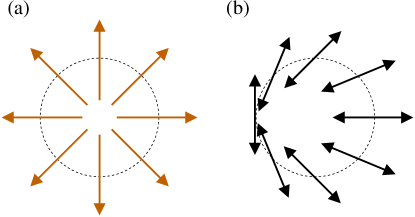
In the presence of the inter-superfluid couplings , no general solution is available. However, considerable insight can be obtained by analyzing limiting regimes. It is clear from the energy density , Eq. (298), that to avoid extensive (scaling with system size) energy cost proportional to (and/or ), the two phases are on average locked together according to
| (302) |
Hence the energy is minimized when positions of the atomic and molecular vortices coincide, and their topological charges (winding numbers) are related by . Thus an elementary vortex in the atomic order parameter will be accompanied by a spatially coincident molecular vortex of topological charge that is double its elementary value, .
In contrast, an elementary molecular vortex is energetically significantly more costly due to incompatibility of the atomic order parameter single-valuedness constraint and the Feshbach resonance constraint (302). It is clear that energetically there are two competing, least costly, ways to accommodate this frustration. One, illustrated in Fig. 14(a), is with a spatially coincident half-integer () atomic vortex, that requires that vanish (atomic component of the gas is normal) along a ray emanating from the location of the vortex core, and across which exhibits a jump discontinuity. The cost of such a defect clearly scales linearly with the length, of the defect ray (more generally, as in dimensions) and is dominated by the loss of the condensation energy along the linear defect.

Another competing possibility, illustrated in Fig. 14(b), is an atomic vortex localized on the elementary molecular vortex, but (in contrast to the noninteracting case where the vortex is isotropic with ) the atomic phase winding is highly anisotropic, with
| (303) | |||||
outside a narrow domain wall strip. The atomic phase makes up the remaining deficit angle (required by single-valuedness of the atomic order parameter), by rapidly winding across the domain wall of width set by and a combination of phase stiffnesses .
It is clear that the first scenario is the limiting case of the second configuration, with large and small , such that the wall width is microscopic (formally smaller than ) and the corresponding energy comparable to condensation energy, thus driving the discontinuity ray normal. The resulting energy in both cases clearly grows linearly (as in dimensions) with the length of the domain wall ray, and the energy scale is set by the minimum of the condensation energy or line tension, with the latter given by the geometrical mean of and a combination of the (see below).
IX.1.2 Domain walls in the ASF
It has been argued that the domain wall with energy linear in its length (more generally, growing as its surface area in dimensions) is another type of a topological excitation in the ASF. Although in the previous subsection it emerged as a necessary string component of a molecular vortex, the existence of a domain wall excitation can be understood on more general grounds. Quite similar to domain walls in an Ising ferromagnet, here too it is a defect that separates ordered domains associated with two physically distinct configurations of the Ising order parameter in the ASF that spontaneously breaks the symmetry of the MSF state. In terms of phases the two domains correspond to two solutions
| (304) |
of the constraint in (302), that are associated with two values of the atomic order parameter , pictorially illustrated in Fig. 15.

A detailed solution for a domain wall can be straightforwardly worked out. To this end, the key (internal) Josephson nonlinearity associated with the Feshbach resonance is isolated by a convenient change of phase variables to new phase fields and :
| (305) | |||||
| (306) |
corresponding to the in-phase and out-of-phase fluctuations of and phases.
In terms of and , the energy density is given by
| (307) |
with
| (308) | |||||
| (309) | |||||
| (310) |
The corresponding saddle-point equations are given by
| (311) | |||||
| (312) |
Eliminating via (311) reduces (312) to the well-studied sine-Gordon equation for ,
| (313) |
where
| (314) |
For a straight domain wall oriented along , defined by the boundary conditions and , the solution is given by
| (315) |
illustrated in Fig. 15. The domain wall width is given by
| (316) |
The associated and corresponding solutions can now be easily obtained from (311), (305), and (306):
| (317) | |||||
| (318) | |||||
| (319) |
IX.1.3 Point-to-“dumbbell” atomic vortex transition
As is clear from the discussion in Sec. IX.1.1, in the ASF a () atomic elementary vortex is driven by the Feshbach resonance (internal Josephson) coupling to be accompanied by a () molecular double vortex. In the limit where , corresponding to a broad Feshbach resonance, and deep in the ASF state, the two superfluids are strongly coupled, and will behave as a single-component conventional atomic superfluid. Thus the atomic and molecular vortices must spatially coincide. This leads to an isotropic topological defect with energy (measured relative to the background energy of the uniform state) given in 2d by
| (324) |
where
| (325) |
consists of the atomic () and molecular () vortex core energies.
Such a concentric, isotropic vortex configuration minimizes the Feshbach resonance energy. However, because it involves a () molecular vortex that is double the elementary charge, it raises the large-scale part of the kinetic energy by over the energy of a topologically equivalent vortex configuration consisting of two elementary () molecular vortices—see (301). As will be shown below, this can drive the splitting of the double molecular vortex into its elementary constituents. This is driven by the fact that, in the absence of the atomic component, two elementary vortices repel via a potential , where is the separation. On the other hand, as shown in Sec. IX.1.1, in the ASF phase an elementary molecular vortex is driven by the internal Josephson coupling to be accompanied by a ( fractional) atomic vortex and a domain-wall string defect. Thus, in the ASF state the logarithmic repulsion of two molecular vortices is arrested by the confining (Josephson coupling) domain-wall energy that, according to (322), grows linearly with separation . Hence, the energy of a point vortex (consisting of coincident atomic and molecular vortices) must be compared to a topologically equivalent “dumbbell” configuration split by a separation into two units, each consisting of coinciding atomic and molecular vortices—see Fig. 5.KV04
The energy of the dumbbell configuration is estimated as
where the core energy is
| (328) |
The first two logarithmic terms in (LABEL:Edumbbell1) estimate the energy associated with the total atomic and total molecular topological charges outside the dumbbell of size . The second two logarithmic terms in (LABEL:Edumbbell1) give the energy of two atomic vortices and two molecular vortices, including their repulsive interaction at separation . Finally, the last term accounts for the energy of the domain wall in the atomic superfluid. Accuracy of the estimate requires that the system size be much larger than the dumbbell size, which in turn must be larger than the microscopic scale: .
To estimate the optimum size of the dumbbell vortex configuration, one minimizes over , yielding
| (329) | |||||
| (330) |
where (323) has been used for , and the estimate in the last line is made by ignoring depletion effects, valid in the dilute, weakly interacting limit.
It is clear that there is a range of parameters and such that the energy , Eq. (LABEL:Edumbbell2), of the dumbbell vortex is lower than that, Eq. (324), of the point vortex configuration. In this case, a 2d system will undergo a transition to a state in which the atomic vortices are in a dumbbell configuration (locked to a molecular vortex pair). Because there is no symmetry change associated with a transition into a state where vortex dumbbells are randomly oriented, one expects this transition to generically be first order.nematicVortex Since the energy balance between the two competing states involves core energies, a more detailed microscopic analysis (that is not pursued here) is necessary to pinpoint the location of the transition. However, it is clear from the structure of and , that such transition takes place for a sufficiently large domain-wall width , where the line tension is small and same-sign vortex repulsion is large. One thus expects such a transition in narrow (small ) Feshbach resonance systems.
IX.2 ASF-MSF as a confinement-deconfinement transition
Observe that the atomic condensate density vanishes as the detuning decreases towards a critical value . Thus the dumbbell length
| (331) |
diverges along with the associated domain-wall width, . Therefore, the ASF–MSF transition in can be complementarily described as a molecular vortex deconfinement transition. While molecular vortices are confined by a linear potential inside the ASF state, in the MSF state this confining potential (in 2d) is replaced by a much weaker logarithmic potential, that binds each molecular vortex to its oppositely charged partner.foot:Lee
IX.3 Molecular superfluid
Since molecular vortices only appear as neutral dipoles in the MSF phase, the state is characterized by long-range order in the molecular order parameter, (however, as usual in 2d, at finite , itself vanishes, while the molecular helicity modulus, or superfluid density, remains finite). On the other hand, a deconfined domain wall (across which the atomic phase jumps by ) leads to a vanishing of the atomic order parameter, .foot:Lee The MSF state exhibits ordinary molecular point vortices, along with the atomic and molecular Bogoliubov quasiparticles discussed in Sec. VI. It is easy to see that, analogous to the conventional BCS superconductor, here too an atomic Bogoliubov quasiparticle (that is gapped) acquires a phase of upon encircling a molecular vortex. Thus, these two excitations interact strongly with each other, with statistical-like interactions that can be captured by a Chern-Simons field theory.fracBalents
X Summary and Conclusions
In this paper the thermodynamics of a resonant atomic Bose gas has been studied. Working within a two-channel model, formulated in terms of bosonic atoms and their diatomic molecules, the complete phase diagram of the system has been worked out as a function of temperature and detuning, the properties of the phases, and the nature of quantum and classical phase transitions between them, studied. This analysis was supplemented by a variational calculation on a one-channel model, whose salient results appear in Sec. I.2.
A most notable feature is the appearance of two distinct superfluid phases, ASF and MSF, separated by an Ising type transition. These are distinguished by the respective presence and absence of atomic off-diagonal long-range order, atomic (gapped and gapless) Bogoliubov spectra, and the nature of topological excitations. In addition to a distinction based on the atomic momentum occupation number, these phases can be distinguished through the domain wall excitations in the ASF (which separate regions in which the atomic phase aligns with the molecular phase in the two possible different ways), characteristic of the broken discrete Ising symmetry.
Acknowledgements.
L.R. thanks Victor Gurarie and Subir Sachdev for discussions, and the Kavli Institute for Theoretical Physics for its hospitality during the “Strongly Correlated Phases in Condensed Matter and Degenerate Atomic” workshop, supported in part by the NSF under grant No. PHY05-51164. The authors acknowledge financial support by the NSF under grant No. DMR-0321848 (LR, JP), NIST under the NRC fellowship (JP), and NASA under contract No. NNC04CB23C (PBW).Appendix A Details of connection to polar-nematic ordering
In this Appendix a connection, stated in Sec.III, between the two complex scalar order parameters, characterizing phases of a resonant atomic Bose gas, to those of a vector-tensor model of polar, nematic liquid crystals is elaborated.
In a thermodynamic description, the order parameters are derived from the full free energy density via derivatives with respect to their conjugate fields:
| (332) |
This prescription is unambiguous for the two-species model (16), but in the one-species model (30) or (240), remains to be defined. One expects a molecular composite operator of the form
| (333) |
to play the role of , where is the molecular wavefunction. Therefore, to investigate molecular superfluid ordering, one is motivated to look at the anomalous correlation function foot:molop
| (334) |
Since the fundamental object is a two-point function, one generally lacks a unique definition of the one-point quantity . However, if the molecular size is much smaller than their separation, in the spirit of the coarse graining picture of the molecular operator , one could define
| (335) |
in which the two-particle molecular wavefunction is used to weigh the local volume average.
A complex-scalar atomic superfluid order parameter is clearly isomorphic to a 2d vector order parameter whose components are the averages
| (336) |
of the corresponding conjugate Hermitian operators,
| (337) |
obeying the commutation relation . Phase symmetric combinations of (i.e., products of its complex conjugate with itself) correspond to rotation invariant combinations (i.e., dot products) of . Similarly, one defines the 2d conjugate field vector .
Since the molecular order parameter is fundamentally a two-point correlation function, one is motivated to examine the tensor
in which the symmetric traceless part is given by
| (343) | |||||
and is therefore seen to be precisely equivalent to the anomalous correlation function . The antisymmetric part
| (346) | |||||
and the trace
| (347) |
are given by the real and imaginary parts of the usual (non-anomalous) two point correlation function
| (348) |
and are therefore phase invariant scalars. The information about the molecular order parameter therefore lies entirely in . One similarly defines the conjugate field tensor
| (349) |
By substituting into (335) one obtains a definition of the local tensor order parameter . The following identities now follow:
| (350) |
This demonstrates that the phase invariant combinations in the Ginzburg-Landau free energy correspond to 2d rotation invariant combinations in the vector-tensor representation.
A symmetric traceless tensor order parameter is familiar from a theory of nematic liquid crystals, encoding the headless-arrow nature of the nematic state of anisotropic molecules.deGennes ; ChaikinLubensky Using the “dictionary”, Eqs.(350), in the vector-tensor representation, , , the mean field Hamiltonian (IV) takes the form
| (351) | |||||
representing the theory of an interacting vector and nematic order parameters. In the current scalar superfluid context both have two components, but (351) is clearly not limited to this case. The conjugate field is the analogue of a magnetic field, while is the analogue of a nematic liquid crystal polarization field.
The “double-headedness” of the nematic order parameter is exhibited via the eigenvector decomposition
| (352) |
in which is the order parameter and are orthonormal unit eigenvectors characterizing the nematic order of the MSF. Clearly is invariant under sign reversal of the unit vectors. Thus, although and completely define , both and characterize the same state.
To make contact with the complex molecular order parameter, let , . From (343) one obtains
| (353) | |||||
Thus the eigenvalue is the MSF order parameter magnitude. Although and are equivalent, is uniquely defined.
Inserting (352) into (351), the Feshbach resonance phase coupling () term takes the form
| (354) |
where the representation has been used. The coupling is again clearly invariant under , and represents an alignment between the nematic and polar order parameters, familiar from the theory of polar nematic liquid crystals. deGennes ; ChaikinLubensky
Appendix B Detailed analysis of mean field phase diagram
In this Appendix a more detailed analysis of the mean field phase diagram, summarized in Sec. IV.2, especially Figs. 10 and 11, is presented. To this end, it is convenient to introduce the following scaled quantities:
| (355) | |||||
Substituting these into the mean field Hamiltonian (IV), one obtains the dimensionless form
| (356) | |||||
The scaling has succeeded in reducing the problem to its essentials, removing entirely, and subsuming all interaction strengths into the single parameter . The only free parameters are the two scaled chemical potentials, . One may always choose the phase of so that it is real and non-negative. It is then clear from the last term in (356) that is minimized by taking to also be real and non-negative, consistent with (37). With this input the scaled extremum equations take the form
| (357) | |||||
| (358) |
and lead to the phase diagrams for and shown in Figs. 17 and 18, respectively (and reproduced in Figs. 10 and 11). These results will now be derived in detail.
B.1 ASF free energy in terms of :
One begins by expressing the energy density in terms of alone by using (357) and (358) to eliminate . In the ASF phase (the transition to which, from the N and MSF phases, is the main focus), where , (357) gives
| (359) |
which clearly requires that the right hand side be positive. The resulting condition,
| (360) |
will be important in what follows.
B.2 Continuous transitions:
It follows from (358) that if , then either (normal phase) or (MSF phase, existing only for ). This is the standard result arising from , showing that the N–MSF transition must be continuous, and take place at .
Substituting into (359), one concludes that any continuous N–ASF transition must take place along the line (with ). For , it is easy to check that is locally unstable to nonzero . Hence, if the transition is first order, representing some global instability, it must occur for .
Similarly, substituting into (359), one finds that any continuous ASF–MSF transition must take place along the curve
| (364) |
For it is easy to check that is locally unstable to nonzero . Hence, any first order transition must occur for .

B.3 First order N–ASF transition:
Consider now the possible existence of a first order N–ASF transition. For all coefficients in (362), aside from the constant term , are positive. A positive root therefore exists only for (vanishing as ), and is clearly unique—see the upper panel in Fig. 16. The continuous transition at therefore takes place for , i.e., .
On the other hand, as illustrated in the lower panel of Fig. 16, for , has a local minimum at some positive value of . Thus, for a range of , there will be two non-negative roots, the smaller of which (vanishing at ) corresponds to a maximum of . It is the larger root, existing for a range of positive , that corresponds to the minimum of associated with the ASF state. For this range of positive the transition from the normal state to this ASF minimum must therefore be first order. These considerations hold for both and .

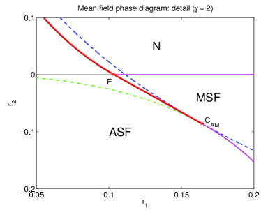
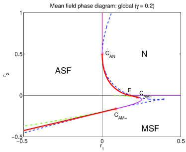
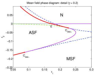
To quantify this, define the cubic discriminant
| (365) |
where
| (366) |
For , has only one real root, while for it has three real roots.foot:cubic As two of the roots merge, and subsequently annihilate as changes sign. There are two branches to the curve (shown as dashed lines in Figs. 17 and 18) given by
| (367) |
of which corresponds to the merging and subsequent disappearance of the two roots of interest. The two branches meet and terminate at a cusp (denoted by a star in Figs. 17 and 18) at the point
| (368) |
where all three roots coincide. The first order transition must therefore take place at a point in the interval where the energy density (362) itself vanishes. For small one finds (the leading quadratic form being exact to all orders for ), and the very small deviation .
B.4 First order MSF–ASF transition:
Along the putative second order line (364), the extremum condition (361) may be factored in the form
| (369) |
in which is the MSF state value, and the other two roots are given by
The argument of the square root is positive, so all three roots are real, and a picture similar to the lower panel of Fig. 16 obtains.
The case :
In order that be the physical root, the condition is required, leading to the inequality
| (371) |
which remains well defined for . Thus, for
| (372) |
the transition is indeed second order. For , becomes the physical root: the transition turns first order, and takes place when the two energy densities match: . The point , is a second tricritical point,BM05 labeled in Fig. 17. At , (369) has a coincident pair of roots, and the line and the transition line must therefore osculate—see Fig. 17.
The case :
For , must be the intermediate root: , leading to the inequality
| (373) |
Thus, for
| (374) |
the transition is indeed second order. For , becomes the physical root, while for , becomes the physical root: in either case the transition turns first order, and takes place when the ASF and MSF energies match. The point , are both tricritical points, labeled in Fig. 18. At both points (369) has a coincident pair of roots, and at both points the (two different branches of the) curve and the transition curve must therefore osculate, as illustrated in Fig. 18. Notice that for , remains well defined, and coincides with , while is pushed to infinity. The semi-infinite second order line is therefore recovered in this limit, consistent with the result.
B.5 Critical endpoint for the N–MSF transition:
Since as , the N–ASF and MSF–ASF first order transition curves must meet at . The second order N–MSF curve also terminates at this point, which therefore represents a critical endpoint, labeled in Figs. 17 and 18.
Figures 17 and 18 show complete phase diagrams, computed for the cases and , respectively, and correspond to the two phase diagram topologies illustrated in Figs. 10 and 11 of the main body of the paper. Here the first order transition curves are computed numerically. The osculation with the line at the various tricritical points is also shown.
Appendix C The two-body molecular binding problem
The center of mass Schrödinger equation for two particles of mass interacting via an attractive potential with microscopic range is given by
| (375) |
Of interest is the regime where the particle is very weakly bound, with binding energy obeying . The wavefunction of such a weakly bound state will extend a distance much greater than outside the potential. A good approximation is then to treat as essentially constant over the potential region (this notion may be made rigorous using effective s-wave scattering parameters). A Fourier analysis of (375) then yields
| (376) |
where is the Fourier transform of the potential, is the area under the potential, and . The self-consistency condition determining is therefore
| (377) |
For the right hand side diverges at . Therefore a bound state solution exists for arbitrarily weak potential. For there is a critical potential strength , below which the potential fails to bind, given by
| (378) |
and one may write
| (379) |
Close to the critical point the integral is dominated by the small region, . One may then ignore the -dependence of (the integral remains convergent for ), to obtain
| (380) |
where
| (381) |
in particular . One therefore obtains the power law relationship describing the vanishing of the binding energy upon approach to the critical point.
Appendix D Thermal and Bose condensate density profiles in a harmonic trap
The most direct probe of a trapped degenerate atomic gas is through its spatial density profile, obtained from a freely expanding cloud. In this Appendix, the details of the density profile calculations for a trapped Bose gas are presented. For the weakly interacting case, the profile is well approximated by the noninteracting expression
| (382) |
with the occupation number , for a Bose gas given by the Bose-Einstein distribution
| (383) |
The single-particle spectrum and normalized wavefunctions are solutions of the single particle Schrödinger equation appropriate to a trapping potential . For a 3d harmonic potential (that for simplicity is taken to be isotropic)
| (384) | |||||
| (385) |
with the th Hermite polynomial, a function of the normalized coordinates (), expressed in units of the quantum oscillator length . The chemical potential, (throughout) is determined by the total atom constraint
| (386) |
In this noninteracting limit, at all atoms go into the lowest single-particle state , forming a Bose-Einstein condensate, with
| (387) |
At finite , a fraction of atoms is thermally excited to higher single-particle states, and
| (388) | |||||
is expressible purely in terms of diagonal elements of the single-particle density matrix for a harmonic oscillator
| (389) |
governed by a single-particle Hamiltonian . The density matrix can be found by solving a diffusion equation in a harmonic potential (or equivalently obtained from analytic continuation of the harmonic oscillator evolution operator) with the “initial” condition of obvious from (389).FeynmanStatMech For one has
| (390) |
where
| (391) | |||||
is the finite-temperature “oscillator length” that reduces to the quantum one at low and the classical (thermal) one, (defined by ) at high .
The sum in , Eq. (388), can be evaluated analytically in various limits. For [valid for all but extremely low , where (387) holds] the sum naturally breaks up into two parts with . The two contributions correspond, respectively, to ranges (“thermal”) and (“quantum”) with determined by . The thermal range is characterized by such that , within which the finite temperature auxiliary oscillator length and the corresponding density matrix can be approximated by their thermal classical forms, giving
where a “cutoff” extended zeta function,
| (393) |
has been defined.
The quantum density contribution is characterized by values of such that , and thus by a zero-temperature oscillator length and the density matrix is given by . The resulting sum is then easily computed, yielding
| (394) |
with amplitude factor
| (395) |
being the number of bosons occupying the single-particle ground state, reduced by the factor .
Eliminating , it is clear that and depend strongly on the ratio of the chemical potential to the trap level spacing , with the former determined by the temperature through the total atom number constraint. For (which corresponds to ), the sum in the expression for , Eq. (LABEL:app:n_Tgeneral), can be extended to infinity, introducing only exponentially small error . The resulting thermal density is then given by the extended zeta function
| (396) | |||||
As expected for , the condensate spatial distribution is still given by the Gaussian expression (394), but with an exponentially small condensate
| (397) |
At high (where the gas is nondegenerate), such that , the thermal (and therefore total) density (396) reduces to a pure Gaussian with thermal width , reflecting the high-temperature Boltzmann statistics
| (398) | |||||
in which the relation has been used to satisfy the particle number constraint.
As is lowered, approaching from above, the magnitude of the chemical potential drops below (remaining negative), and (while the condensate fraction remains vanishingly small) the boson density profile (396) develops a non-Boltzmann peak structure even above :
| (399) |
retaining a Gaussian falloff at large . The small- cusp in , that develops as is approached from above, is rounded on the cutoff length , which for is given by , with .
From the prefactor in it is clear that this thermal form cannot persist to low temperatures, as the volume under drops with . Thus, for even lower temperature, , to accommodate all particles is forced to drop below the level spacing, . In this region, the high terms in (LABEL:app:n_Tgeneral), estimated to be , are no longer exponentially small and the sum can no longer, in general, be extended to infinity. However, for , on length scales longer than the cutoff length , the thermal density , Eq. (LABEL:app:n_Tgeneral), is still well approximated by the extended zeta function in Eq. (396), but with and its small cusp smoothed out on a length scale [following from the condition ].
Correspondingly, the condensate contribution begins to grow for through the growth of the coefficient , Eq. 395. In fact for , and , one has , and the finite fraction of the bosons condensed into the lowest single-particle oscillator Gaussian state (with a narrow width ) are precisely what is required to make up for those that cannot fit into the thermal distribution . Thus for the total atom density profile changes dramatically, developing an easily identifiable bimodal distribution , illustrated in Fig. 1.
As discussed in Sec. V.2, this analysis easily generalizes to the two-component Bose gas (bosonic atoms and molecules) that is the focus of this paper.
Appendix E Details of Bose-BCS MSF–ASF criticality
In this appendix, the critical behavior in the vicinity of the ASF transition line is derived as a function of dimension via an analysis of the integral equations (282) for small deviations .
For one obtains finite values for the derivatives
| (400) |
Higher order derivatives, however, lead to divergent integrals at small . The subtracted integral has leading behavior
| (401) | |||||
where
| (402) |
With the subtractions, the integral converges at both large and small . The vanishing of requires now
| (403) |
and leads to
| (404) |
It is easy to see from (400) that and that this solution is consistent with the requirement that . Similarly, for the density deviation one obtains
| (405) | |||||
For integrals in (400) diverge at small indicating singular dependence on and . This infrared singularity has been isolated by writing
| (406) |
where
| (407) |
where now requires only the single subtraction for convergence at large in this lower dimension. It can be checked that for the derivatives of the subtracted integrals and are finite at the critical point, and so have leading linear dependence on and . The corresponding coefficients are
| (408) |
One obtains again
| (409) |
in which is finite for (note that is the lower critical dimension, below which the phase transition ceases to exist, and so one expects special behavior here). This dominates the linear behavior, and the constraint becomes
| (410) |
which, to leading order, has the solution , and hence
| (411) |
From (408) it is easy to see that , so that (411) is again consistent with . Using (406) and (407), the density deviation is
The singular corrections to the linear behavior may be identified with the energy exponent , where the Gaussian specific heat exponent is (not to be confused with the Feshbach resonance coupling). In a full theory this form would be replaced by the exact Ising exponent.
At the upper critical dimension itself there will be logarithmic corrections. Since is the physically important dimension, it is worth presenting the results for this case as well. One may now express the results in terms of elliptic integrals (see Ref. GR, , pp. 232, 235, 905):
| (413) |
where
| (414) |
At small , hence , using the asymptotics of the elliptic integrals (see Ref. GR, , p. 906), the constraint takes the form
| (415) | |||||
with solution
| (416) |
The density deviation takes the form
References
- (1) H. Feshbach, Ann. Phys. 19, 287 (1962).
- (2) E. Timmermans, P. Tommasini, M. Hussein, and A. Kerman, Phys. Rep. 315, 199 (1999).
- (3) R. Wynar, R. S. Freeland, D. J. Han, C. Ryu, and D. J. Heinzen, Science 287, 1016 (2000).
- (4) E. A. Donley, N.R. Claussen, S.T. Thompson, and C.E. Wieman, Nature 417, 529 (2002).
- (5) S. Jochim, M. Bartenstein, A. Altmeyer, G. Hendl, S. Riedl, C. Chin, J. Hecker Denschlag, and R. Grimm, Science 302, 2101 (2003).
- (6) M. Greiner, C. A. Regal, and D. S. Jin, Nature 426, 537 (2003).
- (7) M. W. Zwierlein, C. A. Stan, C. H. Schunck, S. M. F. Raupach, S. Gupta, Z. Hadzibabic, and W. Ketterle, Phys. Rev. Lett. 91, 250401 (2003).
- (8) J. Bardeen, L. N. Cooper, and J. R. Schrieffer, Phys. Rev. 108, 1175 (1957).
- (9) C. A. R. Sa de Melo, M. Randeria, and J. R. Engelbrecht, Phys. Rev. Lett. 71, 3202 (1993).
- (10) E. Timmermans, K. Furuya, P. W. Milonni, and A. K. Kerman, Phys. Lett. A 285, 228 (2001).
- (11) Y. Ohashi and A. Griffin, Phys. Rev. Lett. 89, 130402 (2002).
- (12) J. N. Milstein, S. J. J. M. F. Kokkelmans and M. J. Holland, Phys. Rev. A 66, 043604 (2002).
- (13) A. V. Andreev, V. Gurarie, and L. Radzihovsky, Phys. Rev. Lett. 93, 130402 (2004).
- (14) Q. Chen, J. Stajic, and K. Levin, Phys. Rep. 412, 1 (2005).
- (15) V. Gurarie and L. Radzihovsky, Annals of Physics 322, 2–119 (2007).
- (16) D. M. Eagles, Phys. Rev. 186, 456 (1969).
- (17) A. J. Leggett, J. Phys. (Paris) Colloq. 41, C7-19 (1980).
- (18) P. Nozieres and S. Schmitt-Rink, J. Low Temp. Phys. 59, 195 (1985).
- (19) Greiner, C. A. Regal and D. S. Jin, Phys. Rev. Lett. 94, 070403 (2005).
- (20) T.-L. Ho, Phys. Rev. Lett. 92, 090402 (2004).
- (21) J. Carlson and Sanjay Reddy, Phys. Rev. Lett. 95, 060401 (2005).
- (22) A. Bulgac, J. E. Drut, and P. Magierski, cond-mat/0701786.
- (23) E. Burovski, N. Prokof’ev, B. Svistunov, and M. Troyer, Phys. Rev. Lett. 96, 160402 (2006).
- (24) Y. Nishida and D. T. Son, Phys. Rev. Lett. 97, 050403 (2006).
- (25) P. Nikolic and S. Sachdev, Phys. Rev. A 75, 033608 (2007).
- (26) M. Y. Veillette, D. E. Sheehy, and L. Radzihovsky, Phys. Rev. A 75, 043614 (2007).
- (27) A summary of our results has appeared in: L. Radzihovsky, J. Park, and P. B. Weichman, Phys. Rev. Lett. 92, 160402 (2004).
- (28) M. W. J. Romans, R. A. Duine, S. Sachdev and H. T. C. Stoof, Phys. Rev. Lett. 93, 020405 (2004).
- (29) The problem of particle and particle pair condensation in a system of attractive bosons was first considered, within a zero temperature variational wavefunction approach, by P. Nozieres and D. Saint James, J. Phys. (Paris) 43 1133 (1982).
- (30) O. Penrose, Phil. Mag. 42, 1373 (1951).
- (31) In the experiments the bound state actually exists in a high vibrational state. Observation of a quasi-equilibrium molecular condensate requires that the lifetime of this state be much larger than collisional equilibration time of the vapor. Only then can the lower vibrational states to which this state must eventually decay be neglected.
- (32) D. S. Petrov, C. Salomon, and G. V. Shlyapnikov, Phys. Rev. Lett. 93, 090404 (2004).
- (33) E. A. Donley, N. R. Claussen, S. L. Cornish, J. L. Roberts, E. A. Cornell, and C. E. Wieman, Nature 412, 295 (2001).
- (34) The stability of the resonant Bose gas model studied here was recently examined in S. Basu and E. J. Mueller, cond-mat/0507460. They show that the ASF phase is unstable if the molecule-molecule and atom-molecule interactions both vanish, , but find that stability is restored for . Consistent with the mean field results presented here, in the latter case they find both first and second order segments to the ASF–MSF transition line with a tricritical point equivalent to in Fig. 2 (or in Fig. 17).
- (35) K. Goral, T. Koehler, S. A. Gardiner, E. Tiesinga and P. S. Julienne, J. Phys. B 37, 3457 (2004).
- (36) C. P. Search and P. Meystre, Phys. Rev. Lett. 93, 140405 (2004).
- (37) R. Wynar, R. S. Freeland, D. J. Han, C. Ryu, and D. J. Heinzen, Science 287, 1016 (2000).
- (38) S. J. J. M. F. Kokkelmans and M. J. Holland, Phys. Rev. Lett. 89, 180401 (2002).
- (39) J. L. Roberts, N. R. Claussen, J. P. Burke, Jr., C. H. Greene, E. A. Cornell, and C. E. Wieman, Phys. Rev. Lett. 81, 5109 (1998).
- (40) V. N. Efimov, Sov. J. Nucl. Phys. 12, 589 (1971).
- (41) The authors thank V. Gurarie for discussion on this point.
- (42) In the noninteracting BEC limit () the ASF will not be accompanied by a molecular condensate as it is for a finite Feshbach resonance coupling. As discussed in Sec. IV.2, for a finite a molecular condensate will necessarily appear in the ASF state, but will be small in the weakly interacting limit.
- (43) S. Folling, A. Widera, T. Miller, F. Gerbier, and I. Bloch, Phys. Rev. Lett. 97, 060403 (2006).
- (44) G. K. Campbell, J. Mun, M. Boyd, P. Medley, A. E. Leanhardt, L. Marcassa, D. E. Pritchard, and W. Ketterle, Science 313, 649 (2006).
- (45) R. A. Barankov, C. Lannert, and S. Vishveshwara, cond-mat/0611126 and references therein.
- (46) It is worth pointing out that the second quantized atom-molecule Hamiltonian (16) is similar to that describing second- and sub-harmonic generation in nonlinear optical systems: the operator corresponds to frequency doubling, while corresponds to parametric down conversion. A physical example is a nonlinear medium placed in a Fabry-Perot cavity. The system is driven coherently at either frequency (leading to frequency doubling) or frequency (leading to sub-harmonic generation), or driven at both. The atomic and molecular field operators, , now correspond to the two cavity modes, and in place of detuning is the (relative) driving amplitude. At critical driving intensity the lasing of the second- or sub-harmonic closely resembles a second order transition. For example, approaching from below the driving threshold of , the solution of vanishing sub-harmonic amplitude becomes unstable and bifurcates into two solutions of opposite phase. This transition is analogous to the breaking of the symmetry in going from molecular to atomic superfluid phases. Both the steady state and non-equilibrium properties of this system have been extensively studied: see, e.g., H. J. Kimble, Quantum fluctuations in quantum optics—squeezing and related phenomena, Les Houches, Session LIII, 1990 (Elsevier, 1992) and references therein.
- (47) C. Orzel, A. K. Tuchman, M. L. Fenselau, M. Yasuda, M. A. Kasevich,Science 291, 2386 (2001).
- (48) I. S. Gradshteyn and I. M. Rhyzhik, Table of Integrals, Series, Products (Academic Press, 1980).
- (49) It will be seen in Sec. IV that this transition may also be driven first order in certain regions of the phase diagram (see Figs.2, 10,11). This possibility has been explored previously within a renormalization group framework,FB97 ; LL04 , where runaway flows generated by the coupling between the incipient atomic order and fluctuations in the molecular order parameter, are interpreted in this fashion. Near the point (critical endpoint) where all three phases meet, this is also found unambiguously even at the mean field level.
- (50) Y. W. Lee and Y. L. Lee, Phys. Rev. B 70, 224506 (2004).
- (51) E. Frey and L. Balents, Phys. Rev. B 55, 1050 (1997).
- (52) J. Stenger, S. Inouye, A. P. Chikkatur, D. M. Stamper-Kurn, D. E. Pritchard, and W. Ketterle, Phys. Rev. Lett. 82, 4569 (1999); D. M. Stamper-Kurn, A. P. Chikkatur, A. Gorlitz, S. Inouye, S. Gupta, D. E. Pritchard, and W. Ketterle, Phys. Rev. Lett. 83, 2876 (1999).
- (53) C. Chin, M. Bartenstein, A. Altmeyer, S. Riedle, S. Jochim, J. Hecker Denschlag, and R. Grimm, Science 305, 1128 (2004).
- (54) C. H. Schunck, Y. Shin, A. Schirotzek, M. W. Zwierlein, W. Ketterle, Science 316, 867 (2007); Y. Shin, C. H. Schunck, A. Schirotzek, W. Ketterle, Phys. Rev. Lett. 99, 090403 (2007).
- (55) G. M. Bruun and G. Baym, Phys. Rev. B 74, 033623 (2006).
- (56) In the presence of a hyperfine interaction, open and closed channels are coupled, and the inter-channel transition is accompanied by (an angular momentum compensating) nuclear spin flip. The coupling of the latter to the external magnetic field is much smaller than that of the electrons (by the ratio of the nuclear to the Bohr magneton) and therefore plays a negligible role in the Feshbach resonance parameters.
- (57) L. D. Landau and E. M. Lifshitz, Quantum Mechanics: non-relativistic theory, Permagon, New York, 1977.
- (58) At low energies the same scattering amplitude structure arises for two atoms interacting through a potential with a large potential barrier separating a short-range attractive minimum from the rapidly decaying repulsive part at infinity. For a sufficiently deep minimum, a (negative energy) bound state (molecule) exists. For a sufficiently shallow minimum, a (positive energy) quasi-bound state exists with a finite lifetime (resonance). However, there is also an intermediate range in which there is no bound state, but the real part of the energy pole is negative, and the metastable molecule interpretation fails.
- (59) D. E. Sheehy and L. Radzihovsky, Annals of Physics 322, 1790 (2007).
- (60) From a renormalization group point of view, one may also think of the two species model as a partially renormalized Hamiltonian in which all fluctuations below the scale of the molecular diameter have been integrated out. It will be seen later that the dissociation amplitude will “dress” the particles with a virtual cloud of pairs that diverges in size as resonance is approached. Thus, such a model captures all further renormalization, including critical fluctuations. In particular, the multi-body parameters in , Eq. 16 should all be treated as constants throughout the neighborhood of the Feshbach resonance.
- (61) Since the operators commute with the operators , the standard derivation of the coherent state formulation goes through essentially without change. See, e.g., J. W. Negele and H. Orland, Quantum Many-Particle Systems (Addison-Wesley, 1988).
- (62) Such an order-parameter classification of the phases by the types of broken symmetries is incomplete. There are systems that exhibit (so-called) “topological” phase transitions, that do not break any global symmetry and therefore are not associated with any local order parameter. Probably the best known example of this is the Kosterlitz-Thouless transition in a two-dimensional XY-model [M. Kosterlitz and D. J. Thouless, J. Phys. C 6, 1181 (1973)], where the ordered phase, while exhibiting a finite supefluid density and power-law correlations (that distinguish it from the fully disordered paramagnetic state) does not break any global symmetries, and is not characterized by a local order parameter.
- (63) J. Zinn-Justin, Quantum Field Theory and Critical Phenomena (Clarendon Press, 2002).
- (64) P. G. de Gennes and J. Prost, The physics of liquid crystals, 2nd edition (Oxford, 1995).
- (65) In 1d, for attractive interactions, the energy functional also admits bright soliton solutions that (for a range of parameters) minimize the energy: V. Gurarie, unpublished. Focusing here on sufficiently large nonresonant repulsive interactions, these inhomogeneous solutions we will be neglected.
- (66) P. M. Chaikin and T. C. Lubensky, Principles of condensed matter physics (Cambridge University Press, 1995).
- (67) L. Radzihovsky and J. Toner, Phys. Rev. Lett. 75, 4752 (1995); Phys. Rev. E 57, 1832 (1998).
- (68) The degenerate Bose fluid regime is characterized by a thermal wavelength that becomes of order the interparticle spacing, i.e., . The critical region is characterized by an even larger correlation length: . For the dilute Bose fluid, characterized by , interactions become important only when . Similarly, one expects shifts in the critical line of order , i.e., . Since, for the ideal gas, , this corresponds to relative shifts in the critical temperature. For a detailed analysis of the crossover between ideal and interacting superfluid criticality, see P. B. Weichman, M. Rasolt, M. E. Fisher and M. J. Stephen, Phys. Rev. B 33, 4632 (1986), as well as Ref. W88, below.
- (69) See, e.g., R. M. Ziff, G. E. Uhlenbeck and M. Kac, Phys. Rep. 32, 169 (1977).
- (70) See, e.g., A. Erdélyi, Higher Transcendental Functions (McGraw-Hill, New York, 1953), Vol. 1, Secs. 1.10 and 1.11.
- (71) The – phase diagram, Fig. 2, corresponds to the - phase diagram, Fig. 10 with a constant density constraint applied. As demonstrated in Sec.IV.2, the coupling between the atomic and critical molecular order parameters drives the transition first order (even in mean field theory), leading this point where the three phases meet to be a critical endpoint. The analysis in Sec. V nevertheless remains valid within any of the phases, with still setting a valid reference temperature.
- (72) The nonlinear relation (77) between the canonical and grand canonical variables is an example of the very general feature of Fisher renormalization: see M. E. Fisher, Phys. Rev. 176, 257 (1968). This relation will also be altered by interaction effects very close to the critical line: see footnote WRFS, above.
- (73) M. H. Anderson, J. R. Ensher, M. R. Matthews, C. E. Wieman, and E. A. Cornell, Science 269, 198 (1995).
- (74) K. B. Davis, M.-O. Mewes, M. R. Andrews, N. J. van Druten, D. S. Durfee, D. M. Kurn, and W. Ketterle, Phys. Rev. Lett. 75, 3969 (1995).
- (75) Whether there are three or one gapped modes is a somewhat a semantic question, which comes down to one’s definition of a mode. For example a one-dimensional quantum harmonic oscillator is said to describe one type of quasiparticle. However, from the point of view thermodynamics and symmetry, it is convenient to count this system as having two modes, corresponding to its coordinate and momentum, , , or equivalently creation and annihilation operators, , , associated with a particle and a hole and the fact that it is governed by two (first order) Heisenberg equations.
- (76) The cubic terms in (109) lead to nonzero at higher order, corresponding to corrections to the mean field value of . Such corrections can also be derived from the leading (quadratic) corrections to the free energy—see Sec. VI.4.1.
- (77) More detailed discussion of how the extremum condition for the order parameter mixes different orders in perturbation theory about the weakly interacting limit, and how to ensure consistency order by order for any given quantity, may be found in: P. B. Weichman, Phys. Rev. B 38, 8739 (1988).
- (78) In the presence of a trapping potential, the spectrum should be observably discrete for excitation wavelengths comparable to the system size, and will depend on the trap shape.
- (79) In future work, it might be interesting to revisit the usual Feynman argument that predicts a downturn (roton minimum) in the energy spectrum in the neighborhood of the peak in the structure factor . For the dense fluid there is a strong peak at , the inverse of the mean interparticle spacing, reflecting the oscillation of the density-density correlation function on this scale. For the dilute, weakly interacting fluid this “incipient crystal” structure disappears. However, since the gas parameter can be large near resonance, interesting structure in could return, and in turn generate interesting structure in at higher momenta.
- (80) For a similar analysis may be performed, but one now needs to impose an ultraviolet (large ) cutoff, which physically arises from the vanishing of the scattering coefficients at large .
- (81) P. C. Hohenberg, Phys. Rev. 158, 383 (1967).
- (82) N. D. Mermin and H. Wagner, Phys. Rev. Lett. 17, 1133 (1966).
- (83) M. E. Fisher, M. N. Barber, and D. Jasnow, Phys. Rev. A 8, 1111 (1973).
- (84) In the “hard-spin” description, the Feshbach interconversion term reduces to , locking the atomic phase to the phase of the molecular condensate up to , corresponding to the unbroken symmetry of the MSF. In terms of a vector order parameter, the MSF is characterized by a finite quadrupole moment ( angular harmonic, akin to the nematic, “headless arrow” order in liquid crystals), and ASF by a vector order parameter ( angular harmonic). In this language, in the ASF both the “nematic director” (headless arrow, ) and the vector () are aligned, with their directions locked together. In contrast, in the MSF, while the nematic director is ordered, the vector order is disordered by virtue of only being locked to the nematic director up to an angle . Clearly this unlocking corresponds to a restoration of the Ising symmetry of the MSF. Further discussion of this, and related, issues can be found in Appendix A.
- (85) See, e.g., V. N. Popov, Functional Integrals in Quantum Field Theory and Statistical Physics, (D. Riedel, Dordrecht, 1983), especially Chapter 6.
- (86) The “diamagnetic” nonlinearity, in Eq. (234) is clearly subdominant to . To see that the “paramagnetic” term, is irrelevant it is easiest to integrate out , obtaining a local current-current interaction, that (because of the two extra powers of the gradient) at long wavelengths is subdominant to the local quartic coupling.
- (87) D. J. Bergman and B. I. Halperin, Phys. Rev. B 13, 2145 (1976).
- (88) The connection to a compressible Ising model can be made even closer by a duality transformation. See for example Ref. FB97, .
- (89) B. I. Halperin, T. C. Lubensky, and S. K. Ma, Phys. Rev. Lett. 32, 292 (1974).
- (90) M. E. Fisher, Rev. Mod. Phys. 46, 597 (1974).
- (91) M. Girardeau and R. Arnowitt, Phys. Rev. 113, 755 (1959).
- (92) R. P. Feynman, Statistical Mechanics, Second Edition, (Perseus Books Group 1998).
- (93) Despite this particle gap, it can be shown that the required Goldstone mode appears in the spectrum of the two particle bound states: A. Coniglio and M. Marinaro, Il Nuovo Cimento XLVIII B, 262 (1967).
- (94) The single particle energy spectrum should indeed be gapped in the MSF phase. The fact that it is gapped even in the ASF phase is an artifact of the variational calculation,Nozieres and can be cured by more sophisticated treatments.W88 ; Popov In particular, the usual Bogoliubov approximation for yields gapless excitations, but the variational approach, which includes additional higher order terms in the Hamiltonian coefficients (259) to account for the possibility of molecular order, reopens the gap. Reclosing it requires careful inclusion of further higher order terms.
- (95) M. E. Fisher, Phys. Rev. 176, 257 (1968).
- (96) C. Dasgupta and B. I. Halperin, Phys. Rev. Lett. 47, 1556 (1981).
- (97) For 2d systems that do spontaneously break a continuous symmetry see, for example, L. Radzihovsky, Anisotropic and Heterogeneous Polymerized Membranes, in “Statistical Mechanics of Membranes and Surfaces,” (World Scientific, edited by D. R. Nelson, T. Piran and S. Weinberg), as well as Ref. RTtubules, , and references therein.
- (98) M. P. A. Fisher and D.-H. Lee, Phys. Rev. B 39, 2756 (1989).
- (99) In a different context, this was independently discussed in F. R. Klinkhamer and G. E. Volovik, JETP Lett. 80, 343 (2004).
- (100) The existence of highly anisotropic dumbbell atomic vortices allows for the possibility of liquid crystaldeGennes ; ChaikinLubensky normal phases. These can, in principle, appear when the anisotropic vortices proliferate but exhibit some form of (e.g., smectic or nematic) spatial order, that distinguishes the resulting liquid-crystal normal state from a fully disordered normal state, where vortices form a homogeneous, isotropic liquid.
-
(101)
The physics of the two-component (atom and
molecule two-channel) superfluid model characterized by phases
and coupled by the internal Josephson coupling
(arising from Feshbach resonance) is quite closely related to the
extended xy-model
analyzed by G. Grinstein and D. H. Lee [Phys. Rev. Lett. 55, 541 (1985)]. When is sufficiently large this latter model exhibits fully ordered polar phase where is ordered, a nematic phase where only is ordered (but is not), and a fully disordered, isotropic phase. These are isomorphic to the ASF, MSF and normal phases, respectively, and (as shown by Grinstein and Lee) the polar and nematic phases are separated by an Ising deconfinement transition characterized by the roughenning and loss of line tension of the domain wall across which jumps by ; L. Radzihovsky and J. Park, unpublished. - (102) L. Balents, M. P. A. Fisher, and C. Nayak, Int. J. Mod. Phys. B 12, 1033 (1998); Phys. Rev. B 60, 1654 (1999).
- (103) Similarly, in the microscopic model underlying , in which molecules are formed of bosons with different internal “atomic spin” quantum numbers, the corresponding anomalous average is , in which is Bose field operator for atoms with spin . For example, if free bosons have spin , and must pair with spin to form a molecule, then the atomic order parameter is , while the molecular order parameter must be constructed from .
- (104) The parameters and defined in (365) and (366) are obtained by expressing the cubic equation in the form via the shift . Let , both defined to be real for , and complex conjugates for . Then the exact roots are given by , . For one obtains , .
- (105) R. P. Feynman and A. R. Hibbs, Quantum Mechanics and Path Integrals, (McGraw-Hill, New York, 1965).