Vortex core size in interacting cylindrical nanodot arrays

Abstract

The effect of dipolar interactions among cylindrical nanodots, with a vortex-core magnetic configuration, is analyzed by means of analytical calculations. The cylinders are placed in a $N\times N$ square array in two configurations - cores oriented parallel to each other and with antiparallel alignment between nearest neighbors. Results comprise the variation in the core radius with the number of interacting dots, the distance between them and dot height. The dipolar interdot coupling leads to a decrease (increase) of the core radius for parallel (antiparallel) arrays.

I Introduction

Regular arrays of magnetic particles produced by nanoimprint lithography have attracted strong attention during the last decade. Common structures are arrays of wires, V01 ; NHW+02 cylinders, CKA+99 ; RHS+02 rings, CRE+04 ; RKL+01 and tubes. NCR+05 ; NCM+05 Such structures can be tailored to display different stable magnetized states, depending on their geometric details. Besides the basic scientific interest in the magnetic properties of these systems, there is evidence that they might be used in the production of new magnetic devices or as media for high density magnetic recording. Chou97 In particular, two-dimensional arrays of magnetic nanoparticles have been proposed as candidates for magnetoresistive random access memory (MRAM) devices. Daughton99 ; ZZP00 ; Parkin04

Recent studies on such structures have been carried out with the aim of determining the stable magnetized state as a function of the geometry of the particles. CKA+99 ; RHS+02 ; AAR+02 ; LEA+05 ; PH04 ; ELA+06 In the case of cylindrical particles, three idealized characteristic configurations have been identified: ferromagnetic with the magnetization parallel to the basis of the cylinder, ferromagnetic with the magnetization parallel to the cylinder axis, and a vortex state in which most of the magnetic moments lie parallel to the basis of the cylinder. The occurrence of each of these configurations depends on geometrical factors, such as the linear dimensions and their aspect ratio $\tau\equiv H/R$, with $H$ the height and $R$ the radius of the cylinder. CKA+99 ; RHS+02 ; AAR+02 ; LEA+05 Another issue to be considered is the interaction between particles. In this case the interparticle distance, $D$, is the important parameter. Metlov06 ; LEL+07 ; EAJ+07 Usually $D$ is large enough to make the exchange coupling between particles negligible, making the dipolar interaction a fundamental point concerning the magnetic state of the system. ELA+06 ; PH05

In this paper we focus on cylindrical particles with dimensions such that, in the absence of an external field, the magnetic state is a vortex. For this magnetic configuration the dipolar interaction between the dots is due to the existence of a core region SOH+00 ; WWB+02 in which the magnetic moments have a nonzero component parallel to the cylinder axis. In this case it is relevant to understand how the core magnetization is affected by the interparticle interaction. Recently, Porrati et al. PH05 investigated an array of dots using micromagnetic simulations. In small arrays they observed that the dipolar interaction changes the size of the magnetic core. However, and because of the use of micromagnetic simulations, larger arrays have not been investigated. Therefore, analytical calculations are very desirable to compare with experiments. With this in mind we examine the behavior of the core in arrays of dots in the vortex-core magnetic phase, in configurations with parallel and antiparallel alignment between the cores. We consider analytical calculations based on a continuous description of the dots.Aharoni96

II System & Units

The basic parameters and variables used in our calculations are summarized in figure 1. We consider cylindrical dots with radius $R$ and height, or thickness, $H$, in square arrays with $N\times N$ dots and center-to-center lattice spacing $D$. The distance between any two dots in the array is denoted by $S$. Whenever necessary, cylindrical coordinates $\rho$ and $\phi$ are defined on the dot plane normal to the cylindrical $z$-axis.

The experimental measurement of the vortex core profile and core radius is not a simple task, and usually it is the full core magnetization, $\mu_{z}$, which is measured. SOH+00 ; RSpc With this in mind, the vortex core is characterized through the calculation of an effective core radius, $C_{\mbox{\it\scriptsize eff}}$, defined as the radius of an effective cylinder, uniformly magnetized along its axis, and whose total magnetic moment,

$$\mu_{z}=M_{0}V=M_{0}\pi HC_{\mbox{\it\scriptsize eff}}^{2},$$ (1)

is the same as produced by the $z$-component of the vortex core, as depicted in figure 1. Here $V$ is the dot volume and $M_{0}$ is the saturation magnetization.

Two types of magnetic ordering within the array are examined: all cores parallel (configuration P) and anti-parallel nearest-neighbor cores (configuration AP). This choice is not an arbitrary one, because the P configuration corresponds to the saturated one and the AP configuration is the ground state of the array.

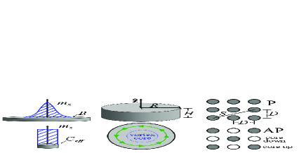
Figure 1: An illustration of geometrical parameters defining each dot and the array.

All linear dimensions will be considered in units of the exchange length $L_{\mbox{\it\scriptsize x}}$, defined as $L_{\mbox{\it\scriptsize x}}=\sqrt{2A/\mu_{0}M_{0}^{2}}$. The dimensionless geometrical parameters are then defined as

$$h\equiv\frac{H}{L_{\mbox{\it\scriptsize x}}},\ r\equiv\frac{R}{L_{\mbox{\it\scriptsize x}}},\ d\equiv\frac{D}{L_{\mbox{\it\scriptsize x}}},\ b=\frac{B}{L_{\mbox{\it\scriptsize x}}},\ c_{\mbox{\it\scriptsize eff}}\equiv\frac{C_{\mbox{\it\scriptsize eff}}}{L_{\mbox{\it\scriptsize x}}},\ s\equiv\frac{S}{L_{\mbox{\it\scriptsize x}}}\,.$$ (2)

III Theoretical model

Large arrays can be studied if we adopt a simplified description of the system in which the discrete distribution of magnetic moments is replaced with a continuous one, defined by a function $\vec{M}(\vec{r})$ such that $\vec{M}(\vec{r})\delta V$ gives the total magnetic moment within the element of volume $\delta V$ centered at $\vec{r}$. Using such a description, the internal energy of the array can be written in terms of the self-energies, $E_{\mbox{\it\scriptsize self}}$, that is, the energies of the isolated dots, and the interaction contribution, $E_{\mbox{\it\scriptsize int}}$, corresponding to the dipolar coupling between the dots. Both $E_{\mbox{\it\scriptsize self}}$ and $E_{\mbox{\it\scriptsize int}}$ have a magnetostatic term given by $E_{\mbox{\it\scriptsize dip}}=(\mu_{0}/2)\int\vec{M}\cdot\nabla U\,dV$ , with $U(\vec{r})$ the magnetostatic potential. Assuming that $\vec{M}(\vec{r})$ varies slowly on the scale of the lattice parameter, the exchange term can be approximated by $E_{\mbox{\it\scriptsize ex}}=A\int\sum(\nabla m_{i})^{2}dV$, where $m_{i}$ is the $i$-th component of the reduced magnetization with respect the saturation value $M_{0}$, that is, $m_{i}=M_{i}/M_{0}$, for $i=x,\ y,\ z$.Aharoni96

III.1 Vortex-core magnetization

For the vortex-core configuration we assume that the magnetization is independent of $z$ and $\phi$, that is,

$$\vec{m}(\vec{r})=m_{z}(\rho){\hat{z}}+m_{\phi}(\rho){\hat{\phi}}\ ,$$ (3)

where $\rho$ is the radial coordinate, $\ {\hat{z}}$ and ${\hat{\phi}}$ are unitary vectors in cylindrical coordinates, and the normalization condition requires that $m_{z}^{2}+m_{\phi}^{2}=1$. The function $m_{z}(\rho)$ specifies the core profile, for which we adopt the model proposed by Landeros et al,LEA+05 given by

$$m_{z}(\rho)=\left[1-(\rho/B)^{2}\right]^{n}\;,\;\ \ 0<\rho<B\;.$$ (4)

and $m_{z}(\rho)=0$ if $B<\rho<R$. Here $B$ is a parameter related to the core radius and the exponent $n$ is a non-negative integer. Alternative expressions for $m_{z}(\rho)$ have been proposed in the literature. FT65 ; UP93 ; Aharoni90 ; HKK03 Figure 2 illustrates the calculated magnetization profile $m_{z}(\rho)$ for a Fe dot ($R=28.2$ nm and $H=37.6$ nm) using different models. The (gray) dash-dotted line corresponds to the model by Usov et alUP93 , the (blue) thin line corresponds to the one proposed by Aharoni,Aharoni90 the (black) thick line corresponds to our modelLEA+05 with $n=4$, the dashed (red) line represents $m_{z}(\rho)$ using the model proposed by Feldtkeller et alFT65 , and the dotted (green) line represents the profile using the model presented by Höllinger et alHKK03 .

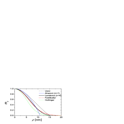
Figure 2: Calculated magnetization profiles, $m_{z}(\rho)$, for different core models. Dimensions are $R=28.2$ nm, $H=37.6$ nm and the material (iron) es defined by $L_{x}=3.327$ nm.

Note that the model proposed by A. AharoniAharoni90 is equivalent to our model (Eq. 4) using $n=1$. We can observe that our model with $n=4$ agrees well with the ones presented in [25] and [28], and has no discontinuities at $m_{z}(\rho=B)=0$, as in the models proposed by Usov et alUP93 and Aharoni,Aharoni90 making the vortex core profile easily integrable. The form for $m_{z}(\rho)$ presented above (Equation (4)) allows us to obtain the magnetization profile by minimizing the total energy of the array. The value of $B$ is determined in the minimization process, as explained below, and the effective core radius ($C_{\mbox{\it\scriptsize eff}}$) can be evaluated equating the $z$-component of total magnetic moment (Equation (1)) with the core magnetic moment, given by

$$\mu_{z}=M_{0}\int_{V}m_{z}(\rho)\rho\,d\rho\,dz\,d\phi\,.$$ (5)

Using the proposed model for $m_{z}(\rho)$, Equation (4), we obtain $\mu_{z}=M_{0}\pi HB^{2}/\left(n+1\right)$ and therefore,

$$C_{\mbox{\it\scriptsize eff}}=\frac{B}{\sqrt{n+1}}\;.$$ (6)

III.2 Total energy calculation

We write all the energies in the dimensionless form, $\tilde{E}=E/\mu_{0}M_{0}^{2}L_{\mbox{\it\scriptsize x}}^{3}$. The energies in the P and AP configurations will be denoted as $\tilde{E}^{+}$ and $\tilde{E}^{-}$, respectively, and can be written as

$$\tilde{E}^{\pm}=N^{2}\tilde{E}_{\mbox{\it\scriptsize self}}+\tilde{E}_{\mbox{\it\scriptsize int}}^{\pm}\;,$$ (7)

where the first term includes the self-energies of the $N^{2}$ isolated dots, and the second term is the interdot magnetostatic coupling.

III.2.1 Self-energy

We consider two contributions to the self-energy, $\tilde{E}_{\mbox{\it\scriptsize self}}$, of an isolate dot in the vortex-core configuration: the dipolar, $\tilde{E}_{\mbox{\it\scriptsize dip}}$, and the exchange, $\tilde{E}_{\mbox{\it\scriptsize ex}}$, contributions. Analytical expressions for the dipolar and exchange energies have been previously calculated by Landeros et al.LEA+05 The dipolar energy results as

$$\tilde{E}_{\mbox{\it\scriptsize dip}}=\pi\alpha_{n}b^{3}-\frac{\pi\beta_{n}b^{4}}{4h}F_{n}\left(b/h\right),$$ (8)

where

$$\alpha_{n}\equiv\frac{2^{2n-1}\Gamma(n+1)^{3}}{\Gamma(n+3/2)\Gamma(2n+5/2)}\,,\quad\beta_{n}\equiv\frac{1}{(n+1)^{2}}$$

and

$$F_{n}(x)=_{P}F_{Q}[(1/2,1,n+3/2),(n+2,2n+3),-4x^{2}]\,.$$

Here, ${}_{P}F_{Q}$ denotes the generalized hypergeometric function, $\Gamma\left(x\right)$ is the gamma function and $n$ corresponds to the exponent used in the core model defined by Equation (4).

For integer values of $n$, the exchange energy reduces to LEA+05

$$\tilde{E}_{\mbox{\it\scriptsize ex}}=\pi h\left[\ln(r/b)+\gamma_{n}\right]\ ,$$ (9)

where $\gamma_{n}=(1/2)\mathcal{H}\left(2n\right)-n\mathcal{H}\left(-1/2n\right)$. Here, $\mathcal{H}\left(z\right)=\sum_{i=1}^{\infty}\left[1/i-1/(i+z)\right]$ is the generalized harmonic number functionEM04 of the complex variable $z$.

III.2.2 Interdot magnetostatic coupling

The dipolar interaction between any two dots in the array depends on the center-to-center distance between them, $S$, and on the relative orientation of the magnetic cores. An expression for this energy is obtained using the magnetostatic field experienced by one of the dots due to the other. Details of these calculations are included in appendix. The resulting expression is

$$\tilde{E}^{\pm}(S)=\pm\frac{2\pi}{L_{\mbox{\it\scriptsize x}}^{3}}\int\limits_{0}^{\infty}dk\,(1-e^{-kH})J_{0}(kS)\left[\int\limits_{0}^{R}J_{0}(k\rho)m_{z}(\rho)\rho d\rho\right]^{2}\,.$$ (10)

Since the size of the core will be obtained by energy minimization, in the previous equation we have considered that the two interacting dots exhibit the same magnetic profile, that is, their cores are identical. Equation (10) allows us to write the interaction energy between two dots as $\tilde{E}^{\pm}(S)=\pm\tilde{E}(S)$, depending on the relative orientation of the cores. Note that if the core size increases, i.e. $m_{z}$ grows, then $\tilde{E}(S)$ increases. Also we always have $\tilde{E}(S)>0$, and the interaction energy between two dots is always greater than zero ($\tilde{E}^{+}(S)>0$) if the cores are oriented in the same direction, which causes a shrinking of the vortex core, in agreement with micromagnetic simulationsPH05 . On the other hand, if the two cores are oriented in opposite directions, then the interaction term is negative ($\tilde{E}^{-}(S)<0$) and the vortex core expands to lower the total energy.

Substituting our expression for $m_{z}\left(\rho\right)$, Equation (4), we obtain

$$\tilde{E}(s)=2^{2n+1}\pi\Gamma^{2}(n+1)\frac{h^{2n+1}}{b^{2n-2}}\\ \int\limits_{0}^{\infty}\frac{dy}{y^{2n+2}}(1-e^{-y})J_{0}\left(y\frac{s}{h}\right)J_{n+1}^{2}\left(y\frac{b}{h}\right)\,.$$ (11)

Using equation (11) and adding up contributions over the entire array we obtain the expression for the total interaction energy of the $N\times N$ square array as

$$\tilde{E}_{\mbox{\it\scriptsize int}}^{\pm}(N)=2N\sum_{p=1}^{N-1}(N-p)(\pm 1)^{p}\tilde{E}(pd)\\ +2\sum_{p=1}^{N-1}\sum_{q=1}^{N-1}(N-p)(N-q)(\pm 1)^{p-q}\tilde{E}\left(d\sqrt{p^{2}+q^{2}}\right).$$ (12)

This equation was previously obtained by Laroze et al, LEL+07 and has been used to investigate the magnetostatic coupling in arrays of magnetic nanowires.

At this point we need to specify the value of the parameter $n$ for the core profile defined by equation (4). In a previous work, Landeros et al LEA+05 showed that the magnetic vortex core can be well described for almost any value of $n>1$. We choose $n=4$, as explained in [14], and finally obtain the following expression for the self-energy,

$$\tilde{E}_{\mbox{\it\scriptsize self}}=0.0298\pi b^{3}-\frac{\pi b^{4}}{100h}F_{4}({b}/{h})+\pi h\left(\ln\frac{r}{b}+2.266\right),$$ (13)

with

$$F_{4}(x) = -\frac{1}{63x^{10}}(256+384x^{2}+576x^{4}$$

$$+600x^{6}+350x^{8}-256F_{21}(-9/2,1/2,6,-4x^{2}))\,,$$

where $F_{21}(a,b,c,z)$ is a hypergeometric function.

Using $n=4$ in Eq. (11) we obtain

$$\tilde{E}(s)=294912\frac{\pi h^{9}}{b^{6}}\int\limits_{0}^{\infty}\frac{dy}{y^{10}}(1-e^{-y})J_{0}\left(y\frac{s}{h}\right)J_{5}^{2}\left(y\frac{b}{h}\right).$$ (14)

Finally, the total energy of the array is calculated as $\tilde{E}^{\pm}=N^{2}\tilde{E}_{\mbox{\it\scriptsize self}}+\tilde{E}_{\mbox{\it\scriptsize int}}^{\pm}$ , with $\tilde{E}_{\mbox{\it\scriptsize self}}$ given by equation (13) and $\tilde{E}_{\mbox{\it\scriptsize int}}^{\pm}$ given by equations (12) and (14).

To determine the vortex core magnetization, we have to minimize $\tilde{E}^{\pm}$ with respect to $b$. Note that the only term in the expression for the energy which depends on the radius $r$ of the dot is $\tilde{E}_{\mbox{\it\scriptsize self}}$ (see equation (13)). However, the derivative of $\tilde{E}_{\mbox{\it\scriptsize self}}$ with respect to $b$ is independent of $r$, leading to a core size that is independent of the dot radius. LEA+05 ; SOH+00 This follows from the fact that the external region of the dot (a perfect vortex) does not interact with the core (apart from the exchange interaction across the interface between the two regions). That is to say, the equation for $b$ that minimizes the total energy of the vortex configuration is independent of $r$.

IV Results and discussion

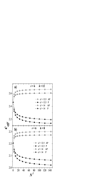
Figure 3: Effective core radius $c_{\mbox{\it\scriptsize eff}}$ vs $N^{2}$ for $r=6$: (a) $h=12$ and (b) $h=8$. Open symbols correspond to an antiparallel (AP) ordering and full symbols to a parallel (P) ordering. Circles correspond to $d=12.5$ and triangles to $d=14$.

We are now in position to investigate how the core radius is affected by the interdot magnetostatic coupling. In order to obtain the value of $b$, the energy $\tilde{E}^{\pm}$ must be minimized for fixed $h$, $d$ and $N$. Since the dipolar interaction is long-ranged, an increment in $N$ leads to an increase in the dipolar field felt by each dot and, therefore, to a change in the core radius until a certain asymptotic value is reached. Figure 3 illustrates this effect for arrays of dots with $r=6$, $d=12.5$ and $14$, and $h=12$ (figure 3(a)) and $h=8$ (figure 3(b)), in configurations P and AP. For both values of $h$ we observe that for $N=12$ the core radius is almost at its limiting size. From our results we observe an increase in the core radius with the number of dots in the AP configuration, and the opposite behavior for the P configuration, in agreement with micromagnetic simulations.PH05 For a given value of $N$, AP arrays with smaller values of $d$ present larger core radius due to the preference for the AP ordering. The antiparallel alignment has the lowest dipolar energy, so the core radius increases with the number of dots in this configuration. On the other hand, in the P configuration the parallel coupling between the cores increases the interaction energy, and then the core region is reduced in order to decrease the interaction.

The dipolar energy may also be varied if the interdot distance is changed. This effect is depicted in figure 4 for the AP and P configurations. While in the antiparallel arrays the size of the core rapidly reaches the value for isolated dots; in the parallel configuration, the effect of the interdot interaction is relevant for longer interdot distances.

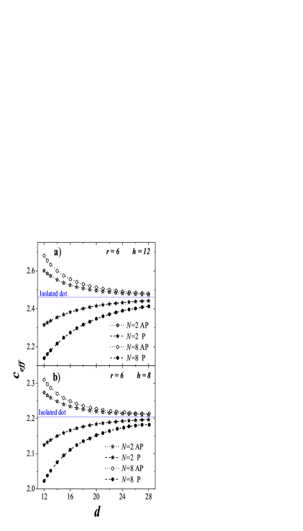
Figure 4: Effective core radius $c_{\mbox{\it\scriptsize eff}}$ vs $d$ for $r=6$: (a) $h=12$ and (b) $h=8$. Open symbols correspond to an antiparallel (AP) ordering and full symbols to a parallel (P) ordering.

Now, the influence of the dot height is more subtle. Figure 5 shows the behavior of $c_{\mbox{\it\scriptsize eff}}$ vs $h$ for arrays of dots with $r=6$, $d=12$, with $N^{2}=4$ and $64$, in the P and AP configurations. For the isolated dot (blue solid line), the effective core follows approximately the relation $c_{\mbox{\it\scriptsize eff}}\approx 1.228+0.291h^{0.577}$.

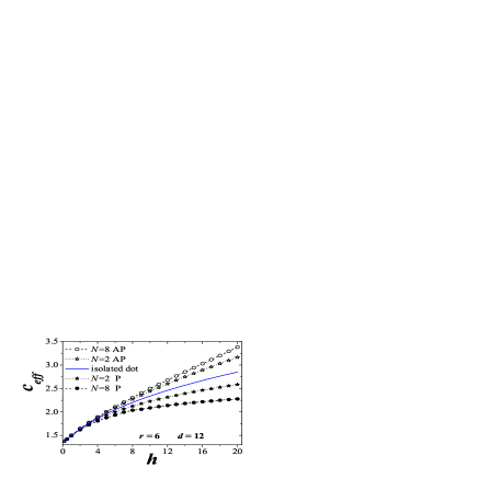
Figure 5: Effective core radius $c_{\mbox{\it\scriptsize eff}}$ vs $h$ for dots with $d=12$, $r=6$. Open symbols correspond to an antiparallel (AP) ordering and full symbols to a parallel (P) ordering. Stars correspond to $N^{2}=4$ and circles to $N^{2}=64$.

For an isolated dot, a transition from the vortex configuration to a complete ferromagnetic ordering along the dot axis is observed as $h$ increases, as shown in the phase diagrams presented in [14]. From the point of view of the core radius, this transition may be seen as a slow and continuous increase in $c_{\mbox{\it\scriptsize eff}}$ with $h$, until $c_{\mbox{\it\scriptsize eff}}\approx r$. As the dots interact in the array this behavior may change. To illustrate this point we calculate the transition line from the out-of-plane uniform state to the vortex-core state configuration in arrays of 4 and 64 dots. The self-energy for the out-of-plane uniform ($u$) state has been presented in TBZ+04 and reads

$$\tilde{E}_{\mbox{\it\scriptsize self}}^{u}=\frac{\pi hr^{2}}{2}\left(1+\frac{8r}{3\pi h}-F_{21}\left[-\frac{4r^{2}}{h^{2}}\right]\right)\ ,$$ (15)

where $F_{21}[x]=F_{21}[-1/2,1/2,2,x]$ is a hypergeometric function.

The interaction energy between two dots with full magnetization along their axis can be obtained from equation (14) using $m_{z}(\rho)=1$ and gives

$$\tilde{E}^{u}(s)=2\pi hr^{2}\int\limits_{0}^{\infty}\frac{dy}{y^{2}}(1-e^{-y})J_{0}(y\frac{s}{h})J_{1}^{2}(y\frac{r}{h})\,,$$ (16)

as presented by Beleggia et al.BTZ+04 The total energy of an array with out-of-plane uniform magnetization is given by

$$\tilde{E}^{u\pm}=N^{2}\tilde{E}_{\mbox{\it\scriptsize self}}^{u}+\tilde{E}_{\mbox{\it\scriptsize int}}^{u\pm}\;,$$ (17)

with the above expressions for the self-energy (equation (15)) and the interaction energy ($\tilde{E}_{\mbox{\it\scriptsize int}}^{u\pm}$) given by equation (12) with the magnetostatic coupling of the two dots given by equation (16). The transition lines between the vortex-core and uniform out-of-plane magnetic states are obtained by equating equations (7) and (17) and are represented in figure 6.

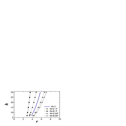
Figure 6: Dipolar induced shifts in the transition line that separates the vortex and the out-of-plane uniform magnetic states. We have fixed the ratio $r/d=0.48$. Open symbols correspond to an antiparallel (AP) ordering and full symbols to a parallel (P) ordering. Stars correspond to $N=2$ and circles to $N=8$.

As we expected, the transition line shifts to lower radii (and greater heights) in the parallel array and to bigger radii (and lower heights) in the antiparallel array. This behavior can be understood by analyzing the interdot dipolar coupling between two dots, $\tilde{E}(s)$. The absolute value of the interaction energy increases with the core size, so $\tilde{E}^{u}(s)>\tilde{E}(s)$, as the uniform out-of-plane ($u$) configuration can be seen as a vortex-core with an infinite core radius, and the magnetostatic coupling for uniform out-of-plane magnetization is stronger than the coupling of two vortex-cores. Therefore, the transition line in a parallel array shifts to the left, because the interactions in an array of vortex-core dots are less than the interactions in a uniformly magnetized P array. On the other hand, in the AP arrays, the interactions are negative and the uniformly magnetized AP configuration is favorable, so the complete ferromagnetic ordering is reached for a smaller value of $h$.

V Conclusions

We have examined the influence of dipolar interactions in the effective core radius of dots in a vortex configuration, placed in an $N\times N$ square array. Dipolar coupling among dots occurs via core interaction, so we consider two types of relative alignment between the cores: parallel, and antiparallel nearest neighbors. Whenever a certain array configuration lowers the interaction energy, the core region expands, as occurs in AP interactions. The opposite behavior occurs for configurations increasing the interaction energy, as the P case. These two orderings represent a demagnetized configuration, the antiparallel case, and a saturated one, corresponding to the parallel case. Effects of the interaction between the dots in the core size have been investigated by varying the number of dots in the array, the distance between them, and their heights. In all cases, an increase of the dipolar interaction energy leads to a decrease of the core radius. When we increase the height of the dots, in the P configuration a transition from vortex to a full ferromagnetic state is hindered, while in the AP configuration the interaction favors the transition to a full AP ferromagnetic state.

Appendix

.

The dipolar interaction energy between two identical dots $i$ and $j$ in the vortex core configuration is given by

$$E_{dip}^{\pm}=\mu_{0}\int_{V_{i}}\vec{M}_{i}(\vec{r})\cdot\nabla U_{j}(\vec{r})\,dV^{\prime}$$

where $\vec{M}_{i}$ is the magnetization of the $i$-th dot and $U_{j}$ is the magnetostatic potential of the $j$-th dot. For the vortex core model defined by Eq. (3)we have $\nabla\cdot\vec{M}=0$, so the magnetostatic potential reduces toLEA+05

$$U_{j}(\vec{r})=\frac{1}{4\pi}\sum_{p=-\infty}^{\infty}\int\limits_{0}^{2\pi}e^{ip(\phi-\phi^{\prime})}d\phi^{\prime}\\ \int\limits_{0}^{R}M_{z}(\rho^{\prime})J_{p}(k\rho^{\prime})\rho^{\prime}d\rho^{\prime}\int\limits_{0}^{\infty}J_{p}(k\rho_{j})[e^{-k(H-z)}-e^{-kz}]dk\,.$$ (18)

In this expression we have used the expansionJackson75

$$\frac{1}{\left|\vec{r}-\vec{r}^{\prime}\right|}=\sum_{p=-\infty}^{\infty}e^{ip(\phi-\phi^{\prime})}\int_{0}^{\infty}J_{p}(k\rho)J_{p}(k\rho^{\prime})e^{-k(z_{>}-z_{<})}dk\;.$$ (19)

Here $J_{p}(z)$ are Bessel functions of first kind. The angular integration gives us $\int_{0}^{2\pi}e^{ip(\phi-\phi^{\prime})}d\phi^{\prime}=2\pi e^{ip\phi}\delta_{p,0}$, leading to

$$U_{j}\left(\rho_{j},z\right)=\frac{1}{2}\int_{0}^{R}\rho^{\prime}M_{z}\left(\rho^{\prime}\right)J_{0}(k\rho^{\prime})d\rho^{\prime}\\ \int_{0}^{\infty}J_{0}(k\rho_{j})\left[e^{-k(H-z)}-e^{-kz}\right]dk.$$ (20)

Since the potential has no dependence on $\phi$, the expression for the energy reduces to

$$E^{\pm}=\mu_{0}\int\limits_{0}^{H}\int\limits_{0}^{2\pi}\int\limits_{0}^{R}M_{z}(\rho)\frac{\partial U_{j}(\rho_{j},z)}{\partial z}\rho d\rho d\phi\,dz\,,$$ (21)

and using Eq. (20) it is straightforward to obtain

$$E^{\pm}=\mu_{0}\int\limits_{0}^{2\pi}d\phi\int\limits_{0}^{\infty}dk\int\limits_{0}^{R}J_{0}(k\rho_{j})M_{z}(\rho)\rho d\rho\\ \int\limits_{0}^{R}J_{0}(k\rho^{\prime})M_{z}(\rho^{\prime})(1-e^{-kH})\rho^{\prime}d\rho^{\prime}\,.$$ (22)

We need to evaluate the potential due to dot $j$ on dot $i$ a distance $S$ apart. Then we have to relate the radial coordinates of both dots through the relation

$$\rho_{j}=\sqrt{\rho^{2}+S^{2}-2\rho S\cos(\phi+\beta)}\,,$$

with $\beta$ an arbitrary angle. Using the following identityJackson75

$$J_{0}(k\rho_{j}) = J_{0}\left(k\sqrt{\rho^{2}+S^{2}-2\rho S\cos(\phi+\beta)}\right)$$

$$= \sum_{p=-\infty}^{\infty}e^{ip(\phi+\beta)}J_{p}(k\rho)J_{p}(kS)\,$$

in the expression for the energy (Eq. 22), after the angular integration, we obtain

$$\tilde{E}^{\pm}[S]=\pm\frac{2\pi}{L_{\mbox{\it\scriptsize x}}^{3}}\int\limits_{0}^{\infty}dk(1-e^{-kH})J_{0}(kS)\left[\int\limits_{0}^{R}J_{0}(k\rho)m_{z}(\rho)\rho d\rho\right]^{2}\,.$$ (23)

References

- (1) M. Vázquez, Physica B 299, 302-313 (2001).
- (2) K. Nielsch, R. Hertel, R. B. Wehrspohn, J. Barthel, J. Kirschner, U. Gösele, S. F. Fischer, and H. Kronmüller, IEEE Trans. Magn. 38, 2571 (2002).
- (3) R. P. Cowburn, D. K. Koltsov, A. O. Adeyeye, M. E. Welland, and D. M. Tricker, Phys. Rev. Lett. 83, 1042 (1999).
- (4) C. A. Ross, M. Hwang, M. Shima, J. Y. Cheng, M. Farhoud, T. A. Savas, Henry I. Smith, W. Schwarzacher, F. M. Ross, M. Redjdal, and F. B. Humphrey, Phys. Rev. B 65, 144417 (2002).
- (5) F. J. Castaño, C. A. Ross, A. Eilez, W. Jung, and C. Frandsen, Phys. Rev. B 69, 144421 (2004).
- (6) J. Rothman, M. Kläui, L. Lopez-Diaz, C. A. F. Vaz, A. Bleloch, J. A. C. Bland, Z. Cui, and R. Speaks, Phys. Rev. Lett. 86, 1098 (2001).
- (7) K. Nielsch, F. J. Castaño, C. A. Ross, and R. Krishnan, J. Appl. Phys. 98, 034318 (2005).
- (8) Kornelius Nielsch, Fernando J. Castaño, Sven Matthias, Woo Lee, and Caroline A. Ross, Adv. Eng. Mat. 7, 217-221 (2005).
- (9) S. Y. Chou, Proc. IEEE 85, 652 (1997); G. Prinz, Science 282, 1660 (1998).
- (10) J. M. Daughton, A. V. Pohm, R. T. Fayfield, and C. H. Smith, J. Phys. D 32, R169 (1999).
- (11) J. G. Zhu, Y. Zheng, and Gary A. Prinz, J. App. Phys. 87, 6668 (2000).
- (12) Stuart S. P. Parkin, Christian Kaiser, Alex Panchula, Philip M. Rice, Brian Hughes, Mahesh Samant, and See-Hun Yang, Nat. Mater. 3, 862 (2004).
- (13) J. d’Albuquerque e Castro, D. Altbir, J. C. Retamal, and P. Vargas, Phys. Rev. Lett. 88, 237202 (2002).
- (14) P. Landeros, J. Escrig, D. Altbir, D. Laroze, J. d’Albuquerque e Castro, and P. Vargas, Phys. Rev. B 71, 094435 (2005).
- (15) F. Porrati, and M. Huth, Appl. Phys. Lett. 85, 3157 (2004).
- (16) J. Escrig, P. Landeros, D. Altbir, M. Bahiana, and J. d’Albuquerque e Castro, Appl. Phys. Lett. 89, 132501 (2006).
- (17) Konstantine L. Metlov, Phys. Rev. Lett. 97, 127205 (2006).
- (18) D. Laroze, J. Escrig, P. Landeros, D. Altbir, M. Vázquez, and P. Vargas, Nanotechnology 18, 415708 (2007).
- (19) J. Escrig, D. Altbir, M. Jaafar, D. Navas, A. Asenjo, and M. Vázquez, Phys. Rev. B 75, 184429 (2007).
- (20) F. Porrati, and M. Huth, J. Magn. Magn. Mater. 290, 145-148 (2005).
- (21) T. Shinjo, T. Okuno, R. Hassdrof, K. Shigeto, and T. Ono, Science 289, 930 (2000).
- (22) A. Wachowiak, J. Wiebe, M. Bode, O. Pietzsch, M. Morgenstern, and R. Wiesendanger, Science 298, 577 (2002).
- (23) A. Aharoni, Introduction to the Theory of Ferromagnetism (Oxford: Clarendon, 1996).
- (24) I. V. Roshchin, and I. K. Schuller, private comm.
- (25) E. Feldtkeller, and H. Thomas, Phys. Kondens. Mater. 4, 8 (1965); P. O. Jubert, and R. Allenspach, Phys. Rev. B 70, 144402 (2004).
- (26) N. A. Usov, and S. E. Peschany, J. Magn. Magn. Mater. 118, L290 (1993).
- (27) A. Aharoni, J. Appl. Phys. 68, 2892-2900 (1990).
- (28) R. Höllinger, A. Killinger, and U. Krey, J. Magn. Magn. Mater. 261, 178-189 (2003).
- (29) O. Espinosa, and V. H. Moll, Integral Transforms and Special Functions 15, 101-115 (2004).
- (30) S. Tandon, M. Beleggia, Y. Zhu, and M. De Graef, J. Magn. Magn. Mater. 271, 21 (2004).
- (31) M. Beleggia, S. Tandon, Y. Zhu, and M. De Graef, J. Magn. Magn. Mater. 278, 270 (2004).
- (32) J. D. Jackson, Classical Electrodynamics, 2nd Edition (John Wiley & Sons, 1975).