Coherent, adiabatic and dissociation regimes in coupled atomic-molecular Bose-Einstein condensates

Abstract

We discuss the dynamics of a Bose-Einstein condensate of atoms which is suddenly coupled to a condensate of molecules by an optical or magnetic Feshbach resonance. Three limiting regimes are found and can be understood from the transient dynamics occuring for each pair of atoms. This transient dynamics can be summarised into a time-dependent shift and broadening of the molecular state. A simple Gross-Pitaevskiĭ picture including this shift and broadening is proposed to describe the system in the three regimes. Finally, we suggest how to explore these regimes experimentally.

I Introduction

Optical and magnetic Feshbach resonances Fedichev et al. (1996); Tiesinga et al. (1993) occur when two colliding particles are resonant with a bound state Feshbach (1958). They have been extensively used to probe and control the properties of ultracold atomic gases Köhler et al. (2006). In particular, they give the ability to tune the interaction between atoms, making ultracold gases very useful to test many-body theories for a wide range of interaction strengths, which is generally not possible in other kinds of systems. These resonances also led to the controlled association of atoms into diatomic molecules, a process called photoassociation Jones et al. (2006) in the case of an optical Feshbach resonance. This association is a coherent process and when applied to degenerate gases, it can result in the formation of a Bose-Einstein condensate of molecules, also called molecular condensate Donley et al. (2002); Herbig et al. (2003).

In this work, we discuss the dynamics of an atomic Bose-Einstein condensate which is suddenly coupled to a molecular condensate through an optical or magnetic Feshbach resonance. In the case of an optical resonance, this can be achieved by turning on a laser on resonance between a colliding pair of atoms and an excited bound state. In the case of a magnetic resonance, this can be achieved by suddenly imposing a magnetic field which brings a bound state in resonance with the colliding pair. In both cases, the two-atom system can be effectively described by two channels: the (open) scattering channel where atoms collide through an interaction potential $U(\vec{r})$ and a (closed) molecular channel where the atoms can bind through an interaction potential $U_{m}(\vec{r})$. The vector $\vec{r}$ denotes the relative position of the two atoms. When $\vec{r}$ becomes large, the potential $U(\vec{r})\to 0$ , and the potential $U_{m}(\vec{r})$ goes to the internal energy $E_{m}$. The two channels are coupled by some potential $W(\vec{r})$. In the case of an optical resonance, the two channels correspond to different electronic states and the coupling is due to the laser. In the case of a magnetic resonance, the two channels correspond to different hyperfine states and the coupling is due to hyperfine interaction. With this simple picture of the resonance at the two-atom level, we can write equations for a Bose-Einstein condensate.

II Equations for coupled atomic-molecular condensate

A coupled atomic-molecular Bose-Einstein condensate can be described by time-dependent equations for its cumulants. Truncating to first order as prescribed in Ref. Köhler and Burnett (2002), one obtains the following set of equations Köhler et al. (2003); Gasenzer (2004); Naidon and Masnou-Seeuws (2006):

$$i\hbar\frac{\partial\Psi}{\partial t}(\vec{x}) = H_{x}\Psi(\vec{x})+\int\Psi^{*}(\vec{y})\big{(}U(\vec{x}-\vec{y})\Phi(\vec{x},\vec{y})+W(\vec{x}-\vec{y})\Phi_{m}(\vec{x},\vec{y})\big{)}d^{3}\vec{y}$$ (1)

$$i\hbar\frac{\partial}{\partial t}\Phi^{\prime}(\vec{x},\vec{y}) = (H_{x}+H_{y})\Phi^{\prime}(\vec{x},\vec{y})+U(\vec{x}-\vec{y})\Phi(\vec{x},\vec{y})+W(\vec{x}-\vec{y})\Phi_{m}(\vec{x},\vec{y})$$

$$i\hbar\frac{\partial}{\partial t}\Phi_{m}(\vec{x},\vec{y}) = (H_{x}+H_{y}-i\gamma/2)\Phi_{m}(\vec{x},\vec{y})+U_{m}(\vec{x}-\vec{y})\Phi_{m}(\vec{x},\vec{y})+W(\vec{x}-\vec{y})\Phi(\vec{x},\vec{y})$$

where $\vec{x}$ and $\vec{y}$ are space coordinates, $t$ is the time variable (for clarity, it is omitted but implicitly present as an argument of all functions), $\hbar$ is the reduced Planck’s constant, $H_{x}=-\frac{\hbar^{2}\nabla_{x}^{2}}{2M}+V(x)$ is the one-body Hamiltonian for a single atom ($M$ is the atom mass and $V$ some external trapping potential), $\Psi$ is the condensate wave function, $\Phi_{m}$ is the pair wave function in the closed channel, and $\Phi$ is the pair wave function in the open channel. The function $\Phi^{\prime}(\vec{x},\vec{y})=\Phi(\vec{x},\vec{y})-\Psi(\vec{x})\Psi(\vec{y})$ is the pair cumulant. It corresponds to the deviation of the pair wave function from its noninteracting form, which is a product of two condensate wave functions. We included a loss term $-i\gamma/2$ in the closed channel to account for possible decay by spontaneous emission.

Usually, only one molecular level $\varphi_{m}$ of the potential $U_{m}$ is in resonance with the atomic condensate pairs. Thus, we can write:

$$\Phi_{m}(\vec{x},\vec{y},t)=\Psi_{m}(\vec{R},t)\varphi_{m}(\vec{r})$$ (2)

where $\vec{R}=(\vec{x}+\vec{y})/2$ and $\vec{r}=\vec{y}-\vec{x}$ are the centre-of-mass and relative coordinates. $\Psi_{m}$ is a one-body field corresponding to the molecular condensate wave function, describing the motion of a molecule whose internal state $\varphi_{m}$ satisfies

$$\big{(}-\frac{\hbar^{2}\nabla_{r}^{2}}{M}+U_{m}(\vec{r})\big{)}\varphi_{m}(\vec{r})=(E_{m}-E_{b})\varphi_{m}(\vec{r})$$

where $E_{b}$ is the binding energy associated with the molecular state $\varphi_{m}$. We choose the normalisation $\langle\varphi_{m}|\varphi_{m}\rangle=1$, and call $\Delta=E_{m}-E_{b}$ the detuning from the resonance.

After some approximations detailed in the appendix, we find that $\Psi$ and $\Psi_{m}$ satisfy the closed set of equations:

$$i\hbar\frac{\partial\Psi}{\partial t}(\vec{x}) = \Big{(}-\frac{\hbar^{2}\nabla_{x}^{2}}{2M}+V(\vec{x})+g|\Psi(\vec{x})|^{2}\Big{)}\Psi(\vec{x})+\Psi^{*}(x)\Big{(}1+g\alpha f(t)\Big{)}w\Psi_{m}(\vec{x})$$ (3)

$$i\hbar\frac{\partial\Psi_{m}}{\partial t}(\vec{x}) = \Big{(}-\frac{\hbar^{2}\nabla_{x}^{2}}{4M}+2V(\vec{x})+\Delta-\Delta^{\prime}-i\gamma/2+w^{2}\alpha f(t)\Big{)}\Psi_{m}(\vec{x})+w\Psi(\vec{x})^{2}$$ (4)

where $g$ is the coupling constant for elastic collisions between atoms, $w$ is the coupling constant for atom-molecule conversion, and $\Delta^{\prime}$ is a light shift of the molecular level due to the coupling. For three-dimensional systems, we have

$$\alpha = \pi/2$$

$$f(t) = \frac{1-i}{2\hbar}\Big{(}\frac{M}{h}\Big{)}^{3/2}\frac{1}{\sqrt{t}}$$

The term $w^{2}\alpha f(t)$ can be interpreted as a time-dependent shift and broadening of the molecular level. It is a time-dependent version of the static light shift $\Delta^{\prime}$: when the interaction is switched on, a large shift and broadening of the molecular level appears during some transient regime and then eventually goes to the static value $\Delta^{\prime}$. The reason for the broadening is the loss of molecules into atom pairs. Indeed, during a certain time, the coupling $w$ can dissociate the molecules into the pair continuum instead of dissociating them back to the atomic condensate state, a process called “rogue dissociation” in Ref. Javanainen and Mackie (2002).

III Coherent, adiabatic and dissociation regimes

We now investigate the different regimes that one can get from Eqs. (3-4). These regimes can be identified by the qualitatively different short-time dynamics. At short times, we can neglect the motion of molecules in the trap. We can also write $\frac{\partial}{\partial t}\Psi_{m}(\vec{x},t)\approx(\Psi_{m}(\vec{x},t)-\Psi_{m}(\vec{x},0))/t$. Using this with the initial conditions (26) in Eq. (4), we can solve for $\Psi_{m}(\vec{x})$ and insert it into Eq. (3). We obtain an effective Gross-Pitaevskiĭ equation for the condensate wave function $\Psi$

$$i\hbar\frac{\partial\Psi}{\partial t}(\vec{x})=\Big{(}-\frac{\hbar^{2}\nabla_{x}^{2}}{2M}+V(\vec{x})+\Big{(}g-w^{2}\frac{1+g\alpha f(t)}{\Delta-\Delta^{\prime}-i\gamma/2+w^{2}\alpha f(t)-\frac{i\hbar}{t}}\Big{)}|\Psi(\vec{x})|^{2}\Big{)}\Psi(\vec{x})$$ (5)

In the local density approximation, this equation leads to the familiar rate equation

$$\dot{\rho}(\vec{x},t)=-K(t)\rho(\vec{x},t)^{2}$$ (6)

where $\rho(\vec{x},t)=|\Psi(\vec{x},t)|^{2}$ is the atomic condensate density, and $K(t)$ is a time-dependent rate coefficient

$$K(t)=\frac{2}{\hbar}\mbox{Im}\frac{w^{2}+gw^{2}\alpha f(t)}{\Delta-\Delta^{\prime}-i\gamma/2+w^{2}\alpha f(t)-\frac{i\hbar}{t}}$$ (7)

This rate coefficient depends only on molecular physics parameters $g$, $w$, $\Delta^{\prime}$, and $\gamma$. In fact, it can be shown to derive from the time-dependent two-body theory, except for the term proportional to $f(t)$ in the numerator of $K(t)$. We find that this term can be neglected when we compare with numerical calculations based on Eqs. (19,20,25). This indicates that the term $f(t)$ should be discarded from Eq. (3). Depending on the relative strengths of the terms in the denominator of $K(t)$, the rate coefficient for a fixed detuning goes through three subsequent regimes illustrated in Fig. 1: linear with time (a), square root of time (b) and constant with time (c).

$$K(t) = \frac{2}{\hbar^{2}}w^{2}t\quad\quad\mbox{ for }t\ll t_{w}$$ (8)

$$K(t) = \frac{4}{\pi}\Big{(}\frac{h}{M}\Big{)}^{3/2}\sqrt{t}\quad\mbox{ for }t_{w}\ll t\ll t_{A}$$ (9)

$$K(t) = \frac{2}{\hbar}\mbox{Im}\frac{w^{2}}{\Delta-\Delta^{\prime}-i\gamma/2}\;\mbox{for }t_{A}\ll t$$ (10)

where we define the two-body time scales

$$t_{w} = \frac{1}{(\pi/2)^{2}}\left(\frac{h}{M}\right)^{3}\left(\frac{\hbar}{w}\right)^{4}$$

$$t_{A} = (\pi/2)^{2}\frac{1}{\hbar^{2}}\left(\frac{M}{h}\right)^{3}\frac{w^{4}}{(\Delta-\Delta^{\prime})^{2}+(\gamma/2)^{2}}$$

The first two regimes correspond to transient dynamics of the pairs, while the third regime yields the rate coefficient of the time-independent two-body theory. Note that the second regime might not exist for small coupling $w$, when $t_{w}>t_{A}$. Then the first and third regime are separated by the time scale $t_{\gamma}=\sqrt{t_{w}t_{A}}$.

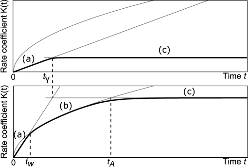
Figure 1: Schematic evolution of the instantaneous rate coefficient (thick black curve) showing the three regimes (a), (b) and (c). Upper graph: moderate coupling ($t_{w}\gtrsim t_{A}$). Lower graph: strong coupling ($t_{w}\ll t_{A}$). The grey curves correspond to the limiting expressions (8,9,10). Note that the parabolic curve associated with Eq. (9) is a universal upper limit of the rate coefficient.

In principle, the two transients regimes (a) and (b) always occur, provided the coupling is large enough. However, they might often occur at very small times, so that they do not affect the system significantly. In other words, the time scales $t_{w}$ and $t_{A}$ might be much smaller than the time scale for the evolution of the gas. We define this time scale as the time $t_{\rho}$ needed to reduce the atomic condensate population by a half. Obviously, this time scale depends on the initial density $\rho_{0}$ of the gas, as can be seen from Eq. (6). Three situations are possible:

• $t_{\rho}\gg t_{A},t_{\gamma}$, in which case the evolution of the gas is governed by the constant rate coefficient (10)

• $t_{w}\ll t_{\rho}\ll t_{A}$, in which case the evolution of the gas is governed by the transient rate coefficient (9)

• $t_{\rho}\ll t_{w},t_{\gamma}$, in which case the evolution of the gas is governed by the transient rate coefficient (8)

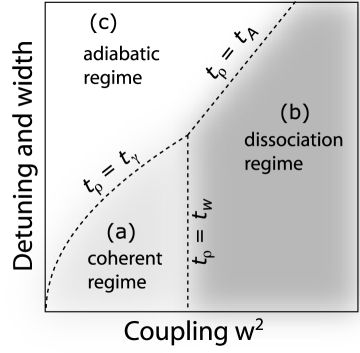
Figure 2: Different regimes of Feshbach resonance in a condensate as a function of the detuning and width $\sqrt{(\Delta-\Delta^{\prime})^{2}+(\gamma/2)^{2}}$ and the coupling strength $w^{2}$, for a fixed density. The boundaries are indicated by dashed lines and equalities of times scales defined in the text.

We call these three situations the adiabatic regime, the dissociation regime and the coherent regime, respectively. They are represented in Fig. 2 for a fixed initial density, as a function of the coupling strength $w^{2}$ and “width and detuning” $\sqrt{(\Delta-\Delta^{\prime})^{2}+(\gamma/2)^{2}}$. In the adiabatic regime, the molecular condensate $\Psi_{m}$ has a very small population because it decays too fast or is too far from resonance and it can be eliminated adiabatically. The system is then described at all times by a single Gross-Pitaevskiĭ equation such as (5). In the dissociation regime, the molecular condensate has also a small population, but now this is because it is dissociated by the coupling into the pair continuum Javanainen and Mackie (2002). The system can be described only in terms of the atomic condensate and dissociated pairs. Interestingly, it is a universal regime in the sense that all quantities depend only upon the mass of the atoms, and not on the particular resonance used. In the coherent regime, the molecular condensate can have a large population and dissociates only into condensate atoms. This creates coherent oscillations between the atomic and molecular condensates, which are described at all times by two coupled Gross-Pitaevskiĭ equations. This regime corresponds to the superchemistry described in Heinzen et al. (2000).

We stress that in all cases, the short-time dynamics of the atomic condensate is described by the rate equation (6) with the time-dependent rate coefficient (7). This shows that the loss of condensate atoms at short times goes like $t$, $t^{3/2}$ and $t^{2}$ for respectively the adiabatic, dissociation, and coherent regimes. For longer times, the system is well described by the two Gross-Pitaevskiĭ equations (3-4) containing the transient shift and broadening. However, higher-order cumulants (quantum fluctuations) neglected in (1), as well as inelastic collisions Yurovsky and Ben-Reuven (2003) between molecules, dissociated pairs or condensate atoms play a role for long times (typically $\sim$10 $\mu$s in the cases shown in Fig. 3).

IV Applications

Experimentally, the adiabatic regime has been well explored with both optical and magnetic Feshbach resonances Cornish et al. (2000); McKenzie et al. (2002); Theis et al. (2004); Winkler et al. (2005). As explained above, the system is then described by a Gross-Pitaevskiĭ equation where the scattering length appearing in the mean-field term is changed by the resonance. In the case of an optical resonance, the scattering length has an imaginary part because of losses from the molecular state by spontaneous emission. These losses are described by the rate equation (6) with the constant rate coefficient (10).

The dissociation regime has proved more difficult to observe. For optical resonances, the losses from the molecular state usually confines the system to the adiabatic regime, as can been seen from Fig. 3. To reach the dissociation regime, one needs to increase the coupling, ie the intensity of the laser. A high-intensity experiment was performed at NIST with a sodium condensate McKenzie et al. (2002), but the laser power was not sufficient to reach the dissociation regime. Experiments in the dissociation regime were performed with magnetic resonances by switching the magnetic field suddenly on or very close to resonance Donley et al. (2001). They resulted in an explosion of hot atoms, and thus were called “Bosenova” experiments. The hot atoms have been identified by several authors with the dissociated pairs discussed above Mackie et al. (2002); Milstein et al. (2003), although several alternative theories exist Duine and Stoof (2001); Santos and Shlyapnikov (2002); Saito and Ueda (2002); Adhikari (2005). Quantitative comparison with any theory has not been completely satisfactory so far Wuester et al. (2007), suggesting that either some element is missing from the theory or some experimental condition has been misunderstood.

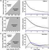
Figure 3: On-resonance photoassociation ($\Delta-\Delta^{\prime}=0$) of a uniform atomic condensate of sodium (a), ytterbium (b) and strontium (c), for typical transitions. In each row, the right panel the time evolution of the populations, according to Eq. (19,20,24), based on the paramaters indicated by the black dot in the left panel, which is a regime diagram similar to Fig. 2. Solid curve: atomic condensate population; dotted curve: dissociated pair population; dot-dashed curve: molecular population. The short-dashed curve shows the atomic and molecular population following from Eqs. (3-4).

We used the following parameters: $w=1.255\cdot 10^{-38}$ J$\cdot\mbox{m}^{3/2}$, $\gamma/\hbar=18$ MHz, $w=3.850\cdot 10^{-39}$ J$\cdot\mbox{m}^{3/2}$, $\gamma/\hbar=364$ kHz for case (b), $w=6.347\cdot 10^{-40}$ J$\cdot\mbox{m}^{3/2}$, $\gamma/\hbar=15$ kHz for case (c). For all three cases, the initial density is $\rho_{0}=6\cdot 10^{14}\mbox{cm}^{-3}$.

To our knowledge, the coherent regime has not been observed. Here we propose to observe the dissociation and coherent regimes by using optical resonances in systems with narrow intercombination lines, for which the molecular states are long-lived. Figure shows the cases of ytterbium and strontium, for typical resonances. In the case of ytterbium, it appears possible to reach the universal regime of dissociation for laser intensities of about 3 W/$\mbox{cm}^{2}$. In the case of strontium for similar intensities, one period of coherent oscillation between the atomic and molecular condensates can be observed.

To illustrate some approximations made in the previous section, we made numerical calculations based on equations (19,20,24) and (3,4) in the case of a uniform system. Fig. 3 shows the evolution of the populations in the atomic, molecular condensate and dissociated pairs. One can see that the short-time dynamics of equations (19,20,24) is well described by the coupled Gross-Pitaevskiĭ equations with the transient shift and broadening, Eqs. (3-4).

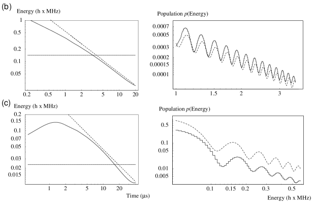
Figure 4: Energy of the noncondensate atoms (dissociated from the molecular state and not returning to the condensate) for the cases (b) and (c) of Fig. 3 (ytterbium and strontium). Note that all graphs are in logarithmic scales. Left panels: average energy as a function of time. For long times, the average energy decreases as $1/t$ curves - the dashed lines are arbitrary $\propto 1/t$ curves shown for reference. Right panel: energy distribution at $t=5\,\mu$s for case (b) and $t=10\,\mu$s for case (c). The dashed curves are obtained from Eq. (11) . The jagged appearance of the curves comes from the numerical discretisation of the pair continuum.

Finally, we present in Fig. 4 the energy distribution of the dissociated pairs for the different systems. In the universal regime, the dissociated pair distribution can be calculated analytically

$$C_{\vec{k}}(\vec{x})=\Big{[}\frac{4}{k^{2}}\sqrt{i\frac{2ht}{M}}-\frac{4\pi i}{k^{3}}\mbox{Erf}\left(k\sqrt{-i\frac{\hbar t}{M}}\right)e^{-i\hbar k^{2}t/m}\Big{]}\Psi(\vec{x})^{2}$$ (11)

where Erf is the error function. From this, one finds the energy distribution $p(E_{k})\propto\frac{M}{4\pi\hbar^{2}}k|C_{k}|^{2}$. Figure 4 shows the average energy of the dissociated pairs as a function of time, and the final energy distribution. Although Eq. (11) is expected to work only at short time and in the universal regime, it gives a good qualitative prediction of the energy distribution (up to a normalisation factor). It is worth noting that when the laser is turned off quickly, although the number of dissociated pairs is maintained, their energy might go down. We find that the laser has to be turned off very fast to maintain the final energy distribution. Therefore there is a range of switch-off speed for which the number of pairs is maintained, while their energy is lowered.

V Conclusion

We showed that three limiting regimes are expected when coupling an atomic condensate to a molecular condensate by an optical or magnetic Feshbach resonance. The three regimes can be identified according to the short-time dynamics of the system. This short-time dynamics can be understood at the two-body level by the transient response of the atom pairs, which is well described by a time-dependent shift and broadening of the molecular state. This shift and broadening can be incorporated into a set of coupled Gross-Pitaevskiĭ equations to describe the short-time dynamics of the system. Finally, we suggested different systems to observe the three regimes experimentally, in particular the universal regime where atom pairs dissociate, and predicted their short-time energy distribution.

VI Appendix

In this appendix, we give the derivation of Eqs. (3-4).

Introduction of coupling constants

We first express the pair cumulant $\Phi^{\prime}$ in terms of centre of mass and relative motion by expanding it over the eigenstates $\varphi_{\vec{k}}(\vec{r})$ of the relative Hamiltonian

$$\Big{(}-\frac{\hbar^{2}\nabla_{r}^{2}}{M}+U(\vec{r})\Big{)}\varphi_{\vec{k}}(\vec{r})=E_{\vec{k}}\varphi_{\vec{k}}(\vec{r}),$$

where $E_{\vec{k}}=\hbar^{2}k^{2}/M$. One can write:

$$\Phi^{\prime}(\vec{x},\vec{y},t)=\Phi^{\prime}(\vec{R},\vec{r},t)=\int\frac{d^{3}\vec{k}}{(2\pi)^{3}}C_{\vec{k}}(\vec{R},t)\varphi_{\vec{k}}(\vec{r}).$$ (12)

For simplicity, only the continuum eigenstates $\varphi_{\vec{k}}(\vec{r})$ of the spectrum are taken into account (the bound states are supposed to be far off-resonant) and we choose the following normalisation: $\langle\varphi_{\vec{k}}|\varphi_{\vec{p}}\rangle=(2\pi)^{3}\delta(\vec{k}-\vec{p})$.

Inserting the decompositions (2) and (12) into the equations (1), one obtains:

$$i\hbar\frac{\partial\Psi}{\partial t}(\vec{x}) = H_{x}\Psi(\vec{x})+\tilde{g}(\vec{x})+\int\Psi^{*}(\vec{r}+\vec{x})\Big{(}U(\vec{r})\int\frac{d^{3}\vec{k}}{(2\pi)^{3}}C_{\vec{k}}(\frac{\vec{r}}{2}+\vec{x})\varphi_{\vec{k}}(\vec{r})+W(\vec{r})\Psi_{m}(\frac{\vec{r}}{2}+\vec{x})\varphi_{m}(\vec{r})\Big{)}d^{3}\vec{r}$$

$$i\hbar\frac{\partial}{\partial t}C_{\vec{k}}(\vec{R}) = (-\frac{\hbar^{2}\nabla_{R}^{2}}{4M}+E_{\vec{k}})C_{\vec{k}}(\vec{R})+\int\frac{d^{3}\vec{q}}{(2\pi)^{3}}v_{\vec{k}\vec{q}}(\vec{R})C_{\vec{q}}(\vec{R})+g_{\vec{k}}(\vec{R})+w_{\vec{k}}\Psi_{m}(\vec{R})$$

$$i\hbar\frac{\partial\Psi_{m}}{\partial t}(\vec{R}) = (-\frac{\hbar^{2}\nabla_{R}^{2}}{4M}+\Delta-i\gamma/2+v_{m}(\vec{R}))\Psi_{m}(\vec{R})+\tilde{w}(\vec{R})+\int\frac{d^{3}\vec{k}}{(2\pi)^{3}}w_{\vec{k}}^{*}C_{\vec{k}}(\vec{R})$$

where

$$\tilde{g}(\vec{x}) = \int\Psi^{*}(\vec{r}+\vec{x})U(\vec{r})\Psi(\vec{x}+\frac{\vec{r}}{2})\Psi(\vec{x}-\frac{\vec{r}}{2})d^{3}\vec{r}$$

$$g_{\vec{k}}(\vec{R}) = \int\varphi_{\vec{k}}(\vec{r})U(\vec{r})\Psi(\vec{R}+\frac{\vec{r}}{2})\Psi(\vec{R}-\frac{\vec{r}}{2})d^{3}\vec{r}$$

$$\tilde{w}(\vec{R}) = \int\varphi_{m}(\vec{r})W(\vec{r})\Psi(\vec{R}+\frac{\vec{r}}{2})\Psi(\vec{R}-\frac{\vec{r}}{2})d^{3}\vec{r}$$

$$w_{\vec{k}} = \int\varphi_{\vec{k}}(\vec{r})W(\vec{r})\varphi_{m}(\vec{r})d^{3}\vec{r}$$

$$v_{m}(\vec{R}) = \int\varphi_{m}(\vec{r})\Big{(}V(\vec{R}+\frac{\vec{r}}{2})+V(\vec{R}-\frac{\vec{r}}{2})\Big{)}\varphi_{m}(\vec{r})d^{3}\vec{r}$$

$$v_{\vec{k}\vec{q}}(\vec{R}) = \int\varphi_{\vec{k}}(\vec{r})\Big{(}V(\vec{R}+\frac{\vec{r}}{2})+V(\vec{R}-\frac{\vec{r}}{2})\Big{)}\varphi_{\vec{q}}(\vec{r})d^{3}\vec{r}$$

are various matrix elements of the couplings $U$,$W$, and $V$ between the states $\Psi$, $\Psi_{m}$ and $C_{\vec{k}}$.

The condensate wave function $\Psi$ and centre-of-mass function $\Psi_{m}$ and $C_{\vec{k}}$ extend over mesoscopic scales, typically up to the micrometre range. On the other hand, quantities such as the interaction potential $U$, $U_{m}$ and the molecular state $\varphi_{m}$ extend over microscopic scales, on the nanometre scale. Therefore, we can make the following approximations

$$\tilde{g}(\vec{x}) \approx \Big{(}\int U(\vec{r})d^{3}\vec{r}\Big{)}\Psi^{*}(\vec{x})\Psi(\vec{x})^{2}\equiv\tilde{g}\Psi^{*}(\vec{x})\Psi(\vec{x})^{2}$$

$$g_{\vec{k}}(\vec{x}) \approx \Big{(}\int\varphi_{\vec{k}}(\vec{r})U(\vec{r})d^{3}\vec{r}\Big{)}\;\;\Psi(\vec{x})^{2}\equiv g_{\vec{k}}\Psi(\vec{x})^{2}$$

$$\tilde{w}(\vec{x}) \approx \Big{(}\int\varphi_{m}(\vec{r})W(\vec{r})d^{3}\vec{r}\Big{)}\;\;\Psi(\vec{x})^{2}\equiv\tilde{w}\Psi(\vec{x})^{2}$$

$$v_{m}(\vec{x}) \approx 2V(\vec{x})$$

which leads to

$$i\hbar\frac{\partial\Psi}{\partial t}(\vec{x}) = H_{x}\Psi(\vec{x})+\Psi^{*}(\vec{x})\Big{(}\tilde{g}\Psi(\vec{x})^{2}+\int\frac{d^{3}\vec{k}}{(2\pi)^{3}}g_{\vec{k}}C_{\vec{k}}(\vec{x})+w_{m}\Psi_{m}(\vec{x})\Big{)}$$ (13)

$$i\hbar\frac{\partial}{\partial t}C_{\vec{k}}(\vec{x}) = \Big{(}-\frac{\hbar^{2}\nabla_{x}^{2}}{4M}+E_{\vec{k}}\Big{)}C_{\vec{k}}(\vec{x})+\int\frac{d^{3}\vec{q}}{(2\pi)^{3}}v_{\vec{k}\vec{q}}(\vec{x})C_{\vec{q}}(\vec{x})+g_{\vec{k}}\Psi(\vec{x})^{2}+w_{\vec{k}}\Psi_{m}(\vec{x})$$ (14)

$$i\hbar\frac{\partial\Psi_{m}}{\partial t}(\vec{x}) = \Big{(}-\frac{\hbar^{2}\nabla_{x}^{2}}{4M}+2V(\vec{x})+\Delta-i\gamma/2\Big{)}\Psi_{m}(\vec{x})+\tilde{w}\Psi(\vec{x})^{2}+\int\frac{d^{3}\vec{k}}{(2\pi)^{3}}w_{\vec{k}}^{*}C_{\vec{k}}(\vec{x})$$ (15)

This is not the most convenient representation for this set of equations, because in the case of a potential $U(\vec{r})$ which is strongly repulsive at short distance, quantities such as $\tilde{g}$ might diverge. Often, one treats this problem by replacing the actual potential $U(\vec{r})$ by a contact pseudopotential $g\delta^{3}(\vec{r})$, where $g$ is adjusted to some relevant finite value. This formally replaces $\tilde{g}$ by $g$, but also introduces ultraviolent divergences, due to the infinitely short range nature of the delta function. One then has to renormalise the coupling constant $g$ using standard techniques in field theory, so as to reproduce physical results. However, in the present case, the whole set of equation is in fact well-behaved with respect to the interaction $U$ and we do not need to resort to such renormalisation techniques, but simply rewrite the equation in another representation.

We decompose $C_{\vec{k}}$ into two contributions, the adiabatic and dynamic ones:

$$C_{\vec{k}}(\vec{x})=C_{\vec{k}}^{ad}(\vec{x})+C_{\vec{k}}^{dyn}(\vec{x})$$

The adiabatic part is defined as the response to the time-dependent source term $g_{\vec{k}}\Psi(\vec{x})^{2}+w_{\vec{k}}\Psi_{m}(\vec{x})$ in Eqs. (14), and is defined as the solution of the system of equations:

$$0=\Big{(}-\frac{\hbar^{2}\nabla_{x}^{2}}{4M}+E_{\vec{k}}\Big{)}C_{\vec{k}}^{ad}(\vec{x})+\int\frac{d^{3}\vec{q}}{(2\pi)^{3}}v_{\vec{k}\vec{q}}(\vec{x})C_{\vec{q}}^{ad}(\vec{x})+g_{\vec{k}}\Psi(\vec{x})^{2}+w_{\vec{k}}\Psi_{m}(\vec{x})$$ (16)

obtained by setting $\partial C_{\vec{k}}/\partial t=0$ in Eq. (14). It is formally solved as

$$C_{\vec{k}}^{ad}(x)=\int\!\!d^{3}\vec{y}\int\!\!d^{3}\vec{q}\;G_{\vec{k}\vec{q}}(\vec{y}-\vec{x})\Big{(}g_{\vec{q}}\Psi(\vec{y})^{2}+w_{\vec{q}}\Psi_{m}(\vec{y})\Big{)}$$ (17)

where $G_{\vec{k}\vec{q}}(\vec{y}-\vec{x})$ is a Green’s function associated with Eq. (16). When introducing $C_{\vec{k}}^{ad}$ in Eqs. (13-14), it appears only in integrals over momenta $\hbar\vec{q}$ where the high-momentum contributions are the most significant. For sufficiently high momenta, we can use a simplified version of (17)

$$C_{\vec{k}}^{ad}(\vec{x})=-\frac{g_{\vec{k}}\Psi(\vec{x})^{2}+w_{\vec{k}}\Psi_{m}(\vec{x})}{E_{\vec{k}}}.$$ (18)

This amounts to neglecting the effects of the trap, i.e. the integral term and the Laplace operator in Eq. (16). Using this expression, we finally obtain

$$i\hbar\frac{\partial\Psi}{\partial t}(\vec{x}) = \Big{(}-\frac{\hbar^{2}\nabla_{x}^{2}}{2M}+V(\vec{x})+g|\Psi(\vec{x})|^{2}\Big{)}\Psi(\vec{x})+\Psi^{*}(x)\Big{(}w\Psi_{m}(\vec{x})+\int\frac{d^{3}\vec{k}}{(2\pi)^{3}}g_{\vec{k}}C_{\vec{k}}^{dyn}(\vec{x})\Big{)}$$ (19)

$$i\hbar\frac{\partial\Psi_{m}}{\partial t}(\vec{x}) = \Big{(}-\frac{\hbar^{2}\nabla_{x}^{2}}{4M}+2V(\vec{x})+\Delta-\Delta^{\prime}-i\gamma/2\Big{)}\Psi_{m}(\vec{x})+w\Psi(\vec{x})^{2}+\int\frac{d^{3}\vec{k}}{(2\pi)^{3}}w_{\vec{k}}^{*}C_{\vec{k}}^{dyn}(\vec{x})$$ (20)

where

$$g = \tilde{g}-\int\!\!\frac{d^{3}\vec{k}}{(2\pi)^{3}}\frac{g_{\vec{k}}^{2}}{E_{\vec{k}}}$$ (21)

$$w = \tilde{w}-\int\!\!\frac{d^{3}\vec{k}}{(2\pi)^{3}}\frac{w_{\vec{k}}g_{\vec{k}}}{E_{\vec{k}}}$$ (22)

$$\Delta^{\prime} = \int\!\!\frac{d^{3}\vec{k}}{(2\pi)^{3}}\frac{w_{\vec{k}}^{2}}{E_{\vec{k}}}$$ (23)

Unlike $\tilde{g}$ and $\tilde{w}$ , the coupling constants $g$ and $w$ are well-defined quantities. The constant $g$ corresponds to the effective interaction strength between condensate atoms (one can show that $g=g_{\vec{0}}=4\pi\hbar^{2}a/M$ where $a$ is the s-wave scattering length associated to the potential $U$). The constant $w$ is the effective coupling between condensate atoms and molecules, and one can show that $w=w_{\vec{0}}$. The quantity $\Delta^{\prime}$ is a shift of the molecular energy due to the atomic-molecular coupling, commonly referred to as “light shift” in the case of an optical resonance.

Equations (19), (20), and Eq. (17) along with the equation

$$i\hbar\frac{\partial}{\partial t}C_{\vec{k}}^{dyn}(\vec{x})=\Big{(}-\frac{\hbar^{2}\nabla_{x}^{2}}{4M}+E_{\vec{k}}\Big{)}C_{\vec{k}}^{dyn}(\vec{x})+\int\frac{d^{3}q}{(2\pi)^{3}}v_{\vec{k}\vec{q}}(\vec{x})C_{\vec{q}}^{dyn}(\vec{x})-i\hbar\frac{\partial}{\partial t}C_{\vec{k}}^{ad}(\vec{x})$$ (24)

form a closed set of equations. Often, $C_{\vec{k}}$ deviates significantly from zero for small $\vec{k}$’s which lie in the Wigner’s threshold law regime Mott and Massey (1965). In this regime, one can make the approximation that $g_{\vec{k}}\approx g$ and $w_{\vec{k}}\approx w$. As a result, the whole set of equations is determined by the three molecular parameters $g$, $w$ and $\Delta^{\prime}$. These quantities can be measured experimentally or calculated from the precise knowledge of the molecular potentials $U$, $U_{m}$ and $W$.

Solution of the equations for an instantaneous coupling

In general, the resolution of Eqs. (19), (20), and (24) is involved and requires numerical calculation. To proceed further, we apply a local density approximation to $C_{\vec{k}}^{dyn}$, namely we neglect again the integral term and the laplacian in Eq. (24),

$$i\hbar\frac{\partial}{\partial t}C_{\vec{k}}^{dyn}(\vec{x})=E_{\vec{k}}C_{\vec{k}}^{dyn}(\vec{x})+\frac{i\hbar}{E_{\vec{k}}}\frac{\partial}{\partial t}\Big{(}g\Psi(\vec{x})^{2}+w\Psi_{m}(\vec{x})\Big{)}$$ (25)

so that the spatial dependence of $C_{\vec{k}}^{dyn}$ comes only from that of $\Psi$ and $\Psi_{m}$. Thus, we make some error regarding the influence of the external trap $V$. This error should be small for times much smaller than the typical oscillation times in the trap. In the following, we will see that the interesting dynamics occurs at the microsecond timescale, while trap oscillations are typically around the millisecond timescale. This approximation is therefore justified.

We are interested in the case where we start from a purely atomic condensate and suddenly turn on the coupling $w$ to a molecular state. The initial conditions are

$$\Psi(\vec{x},0) = \sqrt{\rho_{0}(\vec{x})}$$ (26)

$$\Psi_{m}(\vec{x},0) = 0$$

$$C_{k}^{dyn}(\vec{x},0) = 0$$

where $\rho_{0}(\vec{x})$ is an initial density profile. Integrating Eq. (25) gives

$$C_{\vec{k}}^{dyn}(\vec{x},t)=\int_{0}^{t}e^{\frac{i}{\hbar}E_{k}(\tau-t)}\frac{1}{E_{\vec{k}}}\frac{\partial}{\partial\tau}\Big{(}g\Psi(\vec{x},\tau)^{2}+w\Psi_{m}(\vec{x},\tau)\Big{)}d\tau.$$

This leads to

$$\int\frac{d^{3}\vec{k}}{(2\pi)^{3}}C_{\vec{k}}^{dyn}(\vec{x})=\int_{0}^{t}f(t-\tau)\frac{\partial}{\partial\tau}\Big{(}g\Psi(\vec{x},\tau)^{2}+w\Psi_{m}(\vec{x},\tau)\Big{)}d\tau$$ (27)

with the complex function

$$f(t-\tau) = \int\frac{d^{3}\vec{k}}{(2\pi)^{3}}\frac{e^{\frac{i}{\hbar}E_{k}(\tau-t+i\varepsilon)}}{E_{\vec{k}}}=\frac{1-i}{2\hbar}\Big{(}\frac{M}{2\pi\hbar}\Big{)}^{3/2}\frac{1}{\sqrt{t-\tau}}.$$

The $\varepsilon>0$ is introduced to maintain convergence of the integral. It originates from the momentum dependence of $w_{\vec{k}}$, which we ultimately neglected (which means that $\varepsilon$ is set to zero in the end).

We now assume that the time integral in Eq. (27) is dominated by short-time contributions from $\frac{\partial}{\partial\tau}\Psi_{m}$, which leads to the Ansatz

$$\int_{0}^{t}f(t-\tau)\frac{\partial}{\partial\tau}\Big{(}g\Psi(\vec{x},\tau)^{2}+w\Psi_{m}(\vec{x},\tau)\Big{)}d\tau\approx\alpha f(t)w\Psi_{m}(\vec{x},t)$$ (28)

where $\alpha$ is a numerical factor to be determined. Inserting this result in Eqs. (19-20), we finally get the closed set of equations (3-3).

To determine $\alpha$, we consider the case where the transient shift and broadening is dominant in Eq. (4), which gives

$$\Psi_{m}(\vec{x},t)=\frac{-\Psi(\vec{x},t)^{2}}{w\alpha f(t)}.$$

Inserting this expression in Eq. (28), we find $\alpha=\pi/2$. Interestingly, the same reasoning can be applied to systems of reduced dimensionality, which can be created with an external potential $V(\vec{x})$ strongly confining the atoms in one or two directions Olshanii (1998); Petrov et al. (2000). In this case, the motion of the atoms is frozen in the confined directions. This renormalises the coupling parameters $g$, $w$ and $\Delta^{\prime}$ Naidon and Julienne (2006), and the integration over momenta is reduced to 2 or 1 dimensions in all expressions. For a 2D-like system, we find

$$f_{2D}(t) = \frac{1}{4\pi}\frac{M}{\hbar^{2}}e^{\frac{i}{\hbar}E_{0}t}\Gamma(0,\frac{i}{\hbar}E_{0}t)\sim-\frac{1}{4\pi}\frac{M}{\hbar^{2}}\log(E_{0}t/\hbar)\,\mbox{ for }\,t\ll\hbar/E_{0}$$

$$\alpha_{2D} = 1$$

where $\Gamma$ is the generalised gamma function, and $E_{0}$ is the zero-point energy due to the confinement. For a 1D-like system, however, one finds $\alpha_{1D}=0$, which indicates that the Ansatz is invalid in this case.

References

- Fedichev et al. (1996) P. O. Fedichev, Y. Kagan, G. V. Shlyapnikov, and J. T. M.Walraven, Phys. Rev. Lett. 77, 2913 (1996).
- Tiesinga et al. (1993) E. Tiesinga, B. J. Verhaar, , and H. T. C. Stoof, Phys. Rev. A 47, 4114 (1993).
- Feshbach (1958) H. Feshbach, Ann. Phys. 5, 537 (1958).
- Köhler et al. (2006) T. Köhler, K. Góral, and P. S. Julienne, Rev. Mod. Phys. 78, 1311 (2006).
- Jones et al. (2006) K. M. Jones et al., Rev. Mod. Phys. 78, 483 (2006).
- Donley et al. (2002) E. A. Donley, N. R. Claussen, S. T. Thompson, and C. E. Wieman, Nature 417, 529 (2002).
- Herbig et al. (2003) J. Herbig, T. Kraemer, M. Mark, T. Weber, C. Chin, H.-C. Nägerl, and R. Grimm, Science 301, 1510 (2003).
- Köhler and Burnett (2002) T. Köhler and K. Burnett, Phys. Rev. A 65, 033601 (2002).
- Köhler et al. (2003) T. Köhler, T. Gasenzer, and K. Burnett, Phys. Rev. A 67, 013601 (2003).
- Gasenzer (2004) T. Gasenzer, Phys. Rev. A 70, 043618 (2004).
- Naidon and Masnou-Seeuws (2006) P. Naidon and F. Masnou-Seeuws, Phys. Rev. A 73, 043611 (2006).
- Javanainen and Mackie (2002) J. Javanainen and M. Mackie, Phys. Rev. Lett. 88, 090403 (2002).
- Heinzen et al. (2000) D. J. Heinzen, R. Wynar, P. D. Drummond, and K. V. Kheruntsyan, Phys. Rev. Lett. 84, 5029 (2000).
- Yurovsky and Ben-Reuven (2003) V. A. Yurovsky and A. Ben-Reuven, Phys. Rev. A 67, 043611 (2003).
- Cornish et al. (2000) S. L. Cornish, N. R. Claussen, J. L. Roberts, E. A. Cornell, and C. E. Wieman, 85, 1795 (2000).
- McKenzie et al. (2002) C. McKenzie, J. H. Denschlag, H. Häffner, A. Browaeys, L. E. de Araujo, F. Fatemi, K. M. Jones, J. Simsaran, D. Cho, A. Simoni, et al., Phys. Rev. Lett. 88, 120403 (2002).
- Theis et al. (2004) M. Theis, G. Thalhammer, K. Winkler, M. Hellwig, G. Ruff, R. Grimm, and J. H. Denschlag, Phys. Rev. Lett. 93, 123001 (2004).
- Winkler et al. (2005) K. Winkler, G. Thalhammer, M. Theis, H. Ritsch, R. Grimm, and J. H. Denschlag, Phys. Rev. Lett. 95, 063202 (2005).
- Donley et al. (2001) E. Donley, N. Claussen, S. Cornish, J. Roberts, E. Cornell, and C. Wieman, Nature 412, 295 (2001).
- Mackie et al. (2002) M. Mackie, K.-A. Suominen, and J. Javanainen, Phys. Rev. Lett. 89, 180403 (2002).
- Milstein et al. (2003) J. N. Milstein, C. Menoti, and M. J. Holland, New Journal of Physics 5, 52.1 (2003).
- Duine and Stoof (2001) R. A. Duine and H. T. C. Stoof, Phys. Rev. Lett. 86, 2204 (2001).
- Santos and Shlyapnikov (2002) L. Santos and G. V. Shlyapnikov, Phys. Rev. A 66, 011602(R) (2002).
- Saito and Ueda (2002) H. Saito and M. Ueda, Phys. Rev. A 65, 033624 (2002).
- Adhikari (2005) S. K. Adhikari, Phys. Rev. A 71, 053603 (2005).
- Wuester et al. (2007) S. Wuester, B. J. Dabrowska-Wuester, A. S. Bradley, M. J. Davis, P. B. Blakie, J. J. Hope, and C. M. Savage, Phys. Rev. A 75, 043611 (2007).
- Mott and Massey (1965) N. F. Mott and H. S. W. Massey, Clarendon Press, Oxford, Chap. XIII (1965).
- Olshanii (1998) M. Olshanii, Phys. Rev. Lett. 81, 938 (1998).
- Petrov et al. (2000) D. S. Petrov, M. Holzmann, and G. V. Shlyapnikov, Phys. Rev. Lett. 84, 2551 (2000).
- Naidon and Julienne (2006) P. Naidon and P. S. Julienne, Phys. Rev. A 74, 062713 (2006).