Polarized structure functions of nucleons and nuclei

Abstract

We determine the quark distributions and structure functions for both unpolarized and polarized DIS of leptons on nucleons and nuclei. The scalar and vector mean fields in the nucleus modify the motion of the quarks inside the nucleons. By taking into account this medium modification, we are able to reproduce the experimental data on the unpolarized EMC effect, and to make predictions for the polarized EMC effect. We discuss examples of nuclei where the polarized EMC effect could be measured. We finally present an extension of our model to describe fragmentation functions.

1 Introduction

In order to describe nonperturbative effects like spontaneous chiral symmetry breaking and nuclear binding on the level of quarks, effective chiral quark theories are powerful tools. A prominent example is the EMC effect, which has clearly shown that the quark distributions of bound nucleons differ from those of free nucleons [1]. It has been shown recently [2] that this effect can be explained if one takes into account the response of the quark wave function to the nuclear environment, that is, to the nuclear mean fields, and that the same mechanism gives rise also to medium modifications of the polarized quark distributions and structure functions. In this work, we will focus on the predictions for the polarized EMC effect, and briefly discuss extensions to describe transversity distributions [3] and fragmentation functions [4].

2 Quark distributions and structure functions

In this work we will mainly be concerned with the following EMC ratios:

$$R(x) = \frac{F_{2A}(x_{A})}{ZF_{2p}(x)+NF_{2n}(x)}\,,$$

$$R_{s}^{H}(x) = \frac{g^{H}_{1A}(x_{A})}{P_{p}^{H}g_{1p}(x)+P_{n}^{H}g_{1n}(x)}\,.$$ (1)

Here $x$ is the Bjorken variable for the nucleon, and $x_{A}$ is $A$ times the Bjorken variable for the nucleus of mass number $A$, so that $0<x_{A}<A$. The unpolarized and polarized structure functions of the nucleon are denoted as $F_{2\alpha}$ and $g_{1\alpha}$ respectively ($\alpha=p,n$), while $F_{2A}$ and $g^{H}_{1A}$ are the corresponding structure functions of the nucleus $A$ with spin projection $H=-J,\dots+J$ along the direction of the incoming electron. The polarization factors of protons and neutrons, which appear in the denominator of the spin dependent EMC ratio, are defined as twice the expectation values of the proton and neutron spin operators between the polarized nuclear states. Both ratios in Eq. (1) are defined so that they become unity in a naive single particle model based on nonrelativistic nucleons.

The parton model expressions for the nuclear structure functions are very similar to those of the nucleon [5], for example

$$g_{1A}^{H}(x_{A})=\frac{1}{2}\sum_{q}e_{q}^{2}\,\Delta q_{A}^{H}(x_{A})=\frac{1}{2}\sum_{q}e_{q}^{2}\left(q_{A\uparrow}^{H}(x_{A})-q_{A\downarrow}^{H}(x_{A})\right)\,.$$ (2)

Here $q_{A\uparrow}^{H}(x_{A})$ is the probability to find a quark with momentum fraction $x_{A}/A$ and $s_{z}=1/2$ in the nucleus $A$ with $J_{z}=H$, and similar for $q_{A\downarrow}^{H}(x_{A})$.

It is important to keep in mind the following two points: First, usually only a few valence nucleons (or holes) contribute to the nuclear polarization, and therefore $g_{1A}^{H}$ is of order $1/A$ relative to $F_{2A}$, where all nucleons contribute. Second, the structure function of a free proton is larger and much better known than the neutron structure function. Therefore, possible candidates for the observation of the polarized EMC effect are stable nuclei which are not too heavy, and where the polarization is dominated mainly by the protons.

Nuclear spin sums are interesting quantities, which have not yet been explored in detail. The isoscalar and isovector combinations are

$$\int{\rm d}x_{A}\,\left(\Delta u_{A}^{J}(x_{A})+\Delta d_{A}^{J}(x_{A})\right) = \Sigma\,(P_{p}^{J}+P_{n}^{J})\,,$$

$$\int{\rm d}x_{A}\,\left(\Delta u_{A}^{J}(x_{A})-\Delta d_{A}^{J}(x_{A})\right) = g_{A}\,(P_{p}^{J}-P_{n}^{J})\,,$$ (3)

where we assumed for simplicity that only a single nucleon state contributes to the nuclear polarization. The first relation contains information on the quark spin sum in a bound nucleon ($\Sigma$), and the second one on the axial coupling constant of a bound nucleon ($g_{A}$). The latter is related to nuclear Gamow-Teller matrix elements [6], and establishes an important link between quark physics and nuclear structure physics.

3 Model calculations

We describe the nucleon as a bound state of a quark and a diquark by using the Faddeev framework in the Nambu–Jona-Lasinio (NJL) model. Although the relativistic Faddeev equation, which is represented graphically in Fig. 1, can be solved exactly in the NJL model [7], for our applications to nuclei we limit ourselves to the static approximation, where the momentum dependence of the quark exchange kernel is neglected [8]. We take into account the scalar and axial-vector diquark channels, and avoid unphysical quark decay thresholds by introducing an infrared cut-off, in addition to the ultraviolet one, in the proper-time regularization scheme [9].

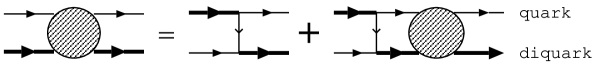
Figure 1: Graphical representation of the Faddeev equation. The single line denotes a quark, and the bold line a diquark.

By using the quark-diquark vertex functions, we evaluate the Feynman diagrams shown in Fig. 2 with the operator insertions $(\gamma_{-},\gamma_{-}\gamma_{5},\gamma_{-}\gamma^{1}\gamma_{5})\times\delta(x-k_{-}/p_{-})$, to get the unpolarized, polarized, and transversity quark distributions, respectively. Here $k$ and $p$ are the momenta of the quark and the nucleon, and $a_{-}$ denotes the light-cone minus-component of a 4-vector $a$. It is straight forward to extend this calculation to the case of a bound nucleon by including the mean nuclear scalar and vector fields into the quark propagators of Fig. 2.

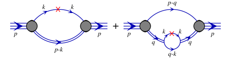
Figure 2: Feynman diagrams for the quark distribution functions in the nucleon. The operators inserted into the quark lines are explained in the text.

Finite nuclei in our present approach are described in a simple independent particle picture: We assume Woods-Saxon scalar and vector potentials for nucleons, with depth parameters determined from our earlier self-consistent nuclear matter calculations [9], and standard values for the range and diffuseness parameters [10]. After solving the Dirac equation with these potentials, we calculate the expectation values of the scalar and vector potentials for each nucleon orbit, and use the quark-diquark (Faddeev) equation to translate them into the average scalar and vector fields for quarks. These average fields are then used in the quark propagators of Fig. 2. Finally, we calculate also the light-cone momentum distributions of the nucleons [2], and obtain the quark distributions in the nucleus by using the convolution formalism.

The parameters of the model are determined as usual from the properties of the pion and the free nucleon. In particular, the 4-Fermi coupling constants in the scalar and axial-vector diquark channels are fitted to the mass and the axial-vector coupling constant of a free nucleon [11]. Then there is only one free parameter in the calculation of the quark distribution functions, which is the model scale ($Q_{0}$) needed to perform the $Q^{2}$ evolution . By fixing this scale to the same value as our constituent quark mass ($400$ MeV), we obtain a very good description of the empirical quark distributions in the free nucleon. This is shown in Figs. 3 and 4, where the results after the $Q^{2}$ evolution (solid lines) are compared to the parametrizations of Refs. [13, 14] (dashed lines). Recently obtained results for the transversity distributions are shown in Ref. [3]. The results are similar to the helicity distributions, which is contrary to the analysis of Ref. [15]. Further investigations on this point are necessary.

Figure 3: Unpolarized valence quark distributions in the free proton.

Figure 4: Polarized valence $u$-distributions (upper part) and $d$-distributions (lower part) in the free proton.

4 Results for nuclear quark distributions and structure functions

In this section we will show our results for the medium modifications of unpolarized and polarized quark distributions and structure functions.

Figure 5: Unpolarized valence $u$-distribution in ¹¹B.

Figure 6: Polarized valence $u$-distribution (upper part) and $d$-distribution (lower part) in ¹¹B.

Fig. 5 shows the unpolarized valence up quark distribution in the nucleus ¹¹B, and Fig. 6 shows the polarized up and down quark distributions for the same nucleus. The dotted lines are the free distributions, i.e., the results obtained by neglecting Fermi motion and medium effects. The dash-dotted lines include the effect of the scalar mean field, the dashed lines include further the Fermi motion, and finally the solid lines incorporate also the effect of the vector mean field.

Comparing the dotted (free result) and the solid (full result) lines in Fig. 5, we see that the unpolarized distribution becomes softer in the nucleus, and that the vector potential plays a very important role to describe this shift to smaller $x$ [16, 17]. The main features shown in Fig. 5, namely a quenching of the distribution function at large $x$ and a small enhancement at smaller $x$, are consistent with the EMC effect. On the other hand, Fig. 6 shows that the polarized quark distributions are quenched in the nucleus for all values of $x$, which implies a reduction of the quark spin sum for a bound nucleon compared to the free nucleon case. In other words, in the medium a part of the quark spin is converted into orbital angular momentum.

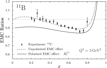
Figure 7: EMC ratios for ¹¹B. The experimental data refer to ¹²C.

The resulting EMC ratios of Eq. (1) for ¹¹B are shown in Fig. 7. It is seen that the polarized EMC effect is predicted to be larger than the unpolarized one. As further possible candidates to measure the polarized EMC effect, we show the results for ⁷Li and ²⁷Al in Figs. 8 and 9. We see that the difference between the two EMC ratios becomes more pronounced as the mass number increases.

The spin sums for the free and the bound nucleon are listed in Table 1. Note that the quantities in the second to fifth columns are defined by dividing out the nuclear polarization factors from the nuclear spin sums (see Eq. (3)), and therefore directly reflect the medium modifications. The last row shows the limit of infinite nuclear matter. We see that the quark spin sums are appreciably quenched in the medium. The last two columns of Table 1 show the tensor charges for the free nucleon [3] and a nucleon bound in infinite nuclear matter.

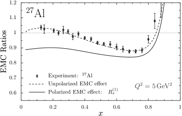
Figure 8: EMC ratios for ²⁷Al.

Figure 9: EMC ratios for ⁷Li. The experimental data refer to ⁹Be.

Table 1: Quark spin sums for a free proton and a proton bound in the nuclear medium.

	$\Delta u$	$\Delta d$	$\Sigma$	$g_{A}$	$\Delta_{T}u$	$\Delta_{T}d$
$p$	0.97	-0.30	0.67	1.27	1.04	-0.24
7Li	0.91	-0.29	0.62	1.19
11B	0.88	-0.28	0.60	1.16
15N	0.87	-0.28	0.59	1.15
27Al	0.87	-0.28	0.59	1.15
nucl. matt.	0.74	-0.25	0.49	0.99	0.93	-0.23

5 Extension to fragmentation functions

Here we wish to discuss a framework to extend the model to fragmentation functions. Numerical results for fragmentation functions will be presented in a future publication [4].

There exists a relation between the quark distribution inside a hadron ($f_{q}^{h}(x)$) and the quark fragmentation function into a hadron ($D_{q}^{h}(z)$), which is known as the Drell-Levy-Yan relation [18]. Let us discuss this relation, starting directly from the operator definitions

$$f_{q}^{h}(x) =\frac{1}{2}\,\hat{\sum}_{n}\,\delta\left(p_{-}x-p_{-}+p_{n-}\right)\left\langle p|\overline{\psi}|p_{n}\right\rangle\gamma^{+}\left\langle p_{n}|\psi|p\right\rangle\,,$$ (4)

$$D_{q}^{h}(z) =\frac{z}{6}\,\frac{1}{2}\,\hat{\sum}_{n}\,\delta\left(\frac{p_{-}}{z}-p_{-}-p_{n-}\right)\left\langle p,\overline{p_{n}}\left|\overline{\psi}\right|0\right\rangle\gamma^{+}\left\langle 0|\psi|p,\overline{p_{n}}\right\rangle\,.$$ (5)

Here $|p\rangle$ denotes the hadron state (we assume a nucleon for definiteness), and $\hat{\sum}_{n}$ is the sum over the intermediate states $|p_{n}\rangle$, including an integral over the momentum and sums over spin and isospin projections. For later convenience, the sum in Eq. (5) is taken over the antiparticle states ($\overline{p_{n}}$).

We can express the matrix element in the distribution function (4) as

$$\langle p_{n}|\psi|p\rangle=\overline{\Gamma}(p,p_{n})\,\sqrt{N_{p}}\,u_{N}({\mbox{\boldmath${p}$}}s)\,,$$ (6)

where the Dirac matrix $\overline{\Gamma}(p,p_{n})$ is the Fourier transform of the Green function $\left\langle p_{n}\left|\left(\psi(0)\overline{\Phi}(x)\right)\right|0\right\rangle$ with $\Phi$ the nucleon field, and $\sqrt{N_{p}}$ is a normalization factor for the nucleon spinor $u_{N}$. Using crossing and charge conjugation symmetries, the matrix element in the fragmentation function (5) can then be expressed as

$$\langle 0|\psi|p,\overline{p_{n}}\rangle=-\sqrt{N_{p}}\overline{v}_{N}({\mbox{\boldmath${p}$}}s)\Gamma(-p,p_{n})\,C$$ (7)

where $C=i\gamma^{2}\gamma_{0}$. Inserting these matrix elements and their conjugates into (4) and (5), it is easy to verify that

$$D_{q}^{h}(z)=\frac{-z}{6}\,f_{q}^{h}\left(x=\frac{1}{z}\right)\biggl{|}_{p\rightarrow-p}\,\,,$$ (8)

where $p\rightarrow-p$ means to reverse all 4 components of $p^{\mu}$, and after this replacement $p^{0}=E_{N}({\mbox{\boldmath${p}$}})>0$.

The effect of the replacement $p\rightarrow-p$ on the distribution function Eq. (4) is seen most easily by expressing it in terms of $\Gamma$ and the quark momentum $k=p-p_{n}$ as follows:

$$f_{q}^{h}(x) =\frac{N_{p}}{8M_{N}}\sum_{n}\int\frac{{\rm d}^{4}k}{(2\pi)^{3}}\,\frac{\Theta(p_{-}(1-x))}{2p_{-}(1-x)}\,\delta\left(k_{+}-e_{N}({\mbox{\boldmath${p}$}})+e_{n}({\mbox{\boldmath${p}$}}-{\mbox{\boldmath${k}$}})\right)$$

$$\hskip 85.35826pt\times\delta(k_{-}-p_{-}x)\ {\rm Tr}\left((\mbox{$\!\not\!p$}+M_{N})\Gamma(p,p-k)\gamma^{+}\overline{\Gamma}(p,p-k)\right),$$

$$\equiv\Theta(1-x)F(x)\,.$$ (9)

Here we expressed the integrand using light-cone variables, and the “energies” of the intermediate state (invariant mass $M_{n}$) and the nucleon are defined by $e_{n}({\mbox{\boldmath${p}$}}_{n})=({\mbox{\boldmath${p}$}}_{n\perp}^{2}+M_{n}^{2})/(2p_{n-})$ and $e_{N}({\mbox{\boldmath${p}$}})=({\mbox{\boldmath${p}$}}_{\perp}^{2}+M_{N}^{2})/(2p_{-})$. From (8) and (9) we obtain finally

$$D_{q}^{h}(z)=-\Theta(1-z)\,\frac{z}{6}\,F\left(x=\frac{1}{z}\right)\,.$$ (10)

(For spin zero bosons, there is no minus sign in Eq. (10).) This shows that $f_{q}^{h}$ and $D_{q}^{h}$ are essentially one and the same function, defined in different regions of the variable. This important result allows us to extend our investigations on the distribution functions presented in this paper to the fragmentation functions. The numerical results and detailed discussions will be presented in a future publication [4].

References

- [1] M. Arneodo, Phys. Rept. 240, 301 (1994); D. F. Geesaman, K. Saito and A. W. Thomas, Ann. Rev. Nucl. Part. Sci. 45, 337 (1995).
- [2] I. C. Cloët, W. Bentz and A. W. Thomas, Phys. Lett. B 642, 210 (2006).
- [3] I. C. Cloët, W. Bentz and A. W. Thomas, arXiv:0708.3246 [hep-ph].
- [4] W. Bentz, T. Ito, A.W. Thomas, and K. Yazaki, to be published.
- [5] R. L. Jaffe and A. Manohar, Nucl. Phys. B 321, 343 (1989).
- [6] A. Arima, K. Shimizu, W. Bentz and H. Hyuga, Adv. Nucl. Phys. 18, 1 (1987).
- [7] N. Ishii, W. Bentz and K. Yazaki, Nucl. Phys. A 587, 617 (1995).
- [8] A. Buck, R. Alkofer and H. Reinhardt, Phys. Lett. B 286, 29 (1992).
- [9] W. Bentz and A. W. Thomas, Nucl. Phys. A 696, 138 (2001) [arXiv:nucl-th/0105022].
- [10] A. Bohr and B.R. Mottelson, Nuclear Structure Vol. 1 (World Scientific, 1998)
- [11] I. C. Cloët, W. Bentz and A. W. Thomas, Phys. Lett. B 621, 246 (2005) [arXiv:hep-ph/0504229].
-
[12]
M. Miyama and S. Kumano,
Comput. Phys. Commun. 94, 185 (1996)
[arXiv:hep-ph/9508246];
M. Hirai, S. Kumano and M. Miyama, Comput. Phys. Commun. 108, 38 (1998) [arXiv:hep-ph/9707220]. - [13] A. D. Martin, R. G. Roberts, W. J. Stirling and R. S. Thorne, Phys. Lett. B 531, 216 (2002) [arXiv:hep-ph/0201127].
- [14] M. Hirai, S. Kumano and N. Saito [Asymmetry Analysis Collaboration], Phys. Rev. D 69, 054021 (2004) [arXiv:hep-ph/0312112].
- [15] M. Anselmino, M. Boglione, U. D’Alesio, A. Kotzinian, F. Murgia, A. Prokudin and C. Turk, Phys. Rev. D 75, 054032 (2007) [arXiv:hep-ph/0701006].
- [16] H. Mineo, W. Bentz, N. Ishii, A. W. Thomas and K. Yazaki, Nucl. Phys. A 735, 482 (2004) [arXiv:nucl-th/0312097].
- [17] W. Detmold, G. A. Miller and J. R. Smith, Phys. Rev. C 73, 015204 (2006) [arXiv:nucl-th/0509033].
- [18] S. D. Drell, D. J. Levy and T. M. Yan, Phys. Rev. 187, 2159 (1969); S. D. Drell, D. J. Levy and T. M. Yan, Phys. Rev. D 1, 1617 (1970).