The impact of Spitzer infrared data on stellar mass estimates – and a revised galaxy stellar mass function at $0<z<5$

Abstract

Aims. We estimate stellar masses of galaxies in the high redshift universe with the intention of determining the influence of newly available Spitzer/IRAC infrared data on the analysis. Based on the results, we probe the mass assembly history of the universe.

Methods. We use the GOODS–MUSIC catalog, which provides multiband photometry from the U–filter to the 8 $\mu m$ Spitzer band for almost $15\,000$ galaxies with either spectroscopic (for $\approx 7\leavevmode\nobreak\ \%$ of the sample) or photometric redshifts, and apply a standard model fitting technique to estimate stellar masses. We than repeat our calculations with fixed photometric redshifts excluding Spitzer photometry and directly compare the outcomes to look for systematic deviations. Finally we use our results to compute stellar mass functions and mass densities up to redshift $z=5$.

Results. We find that stellar masses tend to be overestimated on average if further constraining Spitzer data are not included into the analysis. Whilst this trend is small up to intermediate redshifts $z\la 2.5$ and falls within the typical error in mass, the deviation increases strongly for higher redshifts and reaches a maximum of a factor of three at redshift $z\approx 3.5$. Thus, up to intermediate redshifts, results for stellar mass density are in good agreement with values taken from literature calculated without additional Spitzer photometry. At higher redshifts, however, we find a systematic trend towards lower mass densities if Spitzer/IRAC data are included.

1 Introduction

Whilst the assembly of stellar mass over cosmic history became a matter of interest decades ago, substantial research on this problem has become feasible only in the past few years. Extensive surveys had to be carried out, and techniques to infer stellar masses of galaxies from multicolor photometry had to be developed, as large complete spectroscopic samples at cosmic distances are not yet available. In general, these methods rest upon fitting a grid of stellar population models to the data to compute stellar masses by multiplying the mass–to–light ratio of the best matching template with its absolute luminosity. This procedure has been used in numerous publications to calculate stellar mass functions or stellar mass densities up to intermediate redshifts (e.g. Brinchmann & Ellis 2000; Drory et al. 2001; Bell et al. 2003; Borch et al. 2006). With the increasing availability of deeper surveys, the analysis has been extended to higher redshifts, e.g. up to $z=2$ or 3 (Dickinson et al. 2003b; Fontana et al. 2003; Rudnick et al. 2003; Fontana et al. 2004), or even to $z=5$ (Drory et al. 2005). However, the derived results are typically based on observations from the U to the K–band and may be affected by extrapolation errors as the rest–frame wavelength coverage of the observed objects is shifted to the blue, and a good observational constraint to a galaxy’s optical to near–infrared rest–frame luminosity is necessary to estimate its stellar mass reliably. Results for stellar masses may therefore be impaired by systematic uncertainties in the high redshift regime if observations are not extended to longer wavelengths.

Since the Spitzer space telescope has become operational, it has been possible to complement observations up to the K filter with high–quality infrared data in the adjacent wavelength range (Werner et al. 2004). To benefit from this improvement we used the Great Observatories Origins Deep Survey, which provides deep publicly available observations from numerous facilities in different wavelength regimes (Dickinson et al. 2003a). Based on these data we probe the influence of Spitzer photometry on the estimated stellar masses and examine the consequences of the results on inferences about the mass assembly history of the universe. In this work we address the effects of Spitzer data to the mass calculation process only, i.e. we do not study whether additional systematic deviations of photometric redshifts emerge that, in general, can influence the result as well. Furthermore we adopt a specific set of template models for the calculations.

The paper is organized as follows. In Sect. 2 we give a short overview of the dataset, and discuss the procedure adopted to estimate stellar masses in Sect. 3. We focus on the influence of Spitzer data on the derived masses in Sect. 4 and use the outcome to calculate stellar mass functions (Sect. 5) and mass densities (Sect. 6). Finally, we summarise our results and draw our conclusions in Sect. 7.

Throughout the paper we assume $\Omega_{\mathrm{M}}=0.3$, $\Omega_{\Lambda}=0.7$ and $H_{0}=70\leavevmode\nobreak\ \mathrm{km\,s^{-1}\,Mpc^{-1}}$. Magnitudes are given in the AB system.

2 The dataset

To study the assembly of stellar mass we focus on the Chandra Deep Field South, where numerous observations within the framework of the Great Observatories Origins Deep Survey (GOODS) provide data over a wide range of wavelengths. The present paper is based on GOODS–MUSIC, a multicolor catalog published by Grazian et al. (2006). We briefly discuss its main characteristics here and refer the reader to that paper for a more detailed description.

The catalog combines U–band data from the 2.2m–MPE/ESO telescope and VLT/VIMOS ($\mathrm{U_{35}}$, $\mathrm{U_{38}}$ and $\mathrm{U_{VIM}}$), Hubble/ACS images in F435W (B), F606W (V), F775W (i) and F850LP (z), VLT/ISAAC data in J, H and $\mathrm{K_{S}}$, and Spitzer/IRAC data at $3.6\leavevmode\nobreak\ \mu m$, $4.5\leavevmode\nobreak\ \mu m$, $5.8\leavevmode\nobreak\ \mu m$ and $8.0\leavevmode\nobreak\ \mu m$. Since observations have not yet been finished in all bands, the coverage fraction lies at around 63 % for $\mathrm{U_{VIM}}$–data and at about 54 % for the H–band (ISAAC data release 1.0). Source detection has been performed independently in both the deep z–image (14651 objects detected) and the shallower $\mathrm{K_{S}}$–band data (2931 sources), ending up with a z– and $\mathrm{K_{S}}$–complete catalog consisting of $14\,847$ objects in total. Special software was developed for photometry (De Santis et al. 2006) to meet the requirements of color measurement in combined ground and space based observations with dissimilar point spread functions. Out of all objects, 13767, 12041, 6767 and 5869 sources could be detected in the IRAC data in channels 1, 2, 3 and 4, respectively. For objects undetected in a specific image, upper limits in flux were calculated on the basis of morphological information derived from the detection image. As a last step redshift information were added to complete the dataset. To do this, spectroscopic surveys available at that time were used to assign 1068 spectroscopic redshifts. For the remaining objects, a standard photometric redshift code was applied that was able to reproduce the spectroscopic redshifts with an accuracy of $\langle|\frac{\Delta z}{1+z}|\rangle=0.045$. As shown in Fig. 12 of Grazian et al. (2006), less than 2 % of the spectroscopically observed objects reveal a photometric redshift that deviates severely ($|z_{spec}-z_{phot}|>0.3=5\cdot\langle\sigma\rangle$) from the spectroscopic one.

In summary, the catalog used here consists of $14\,847$ objects enclosing at least 72 stars and 68 AGNs over a total area of 143.2 $\mathrm{arcmin^{2}}$, with mean limiting magnitudes of $\mathrm{z_{lim}}\approx 26.0$ and $\mathrm{K_{S\;lim}}\approx 23.8$ at 90 % completeness level.

3 Deriving stellar masses

To calculate galaxy stellar masses we adopted the method described in Drory et al. (2004a) and locally tested against spectroscopic results in Drory et al. (2004b). This method is based on comparing object colors to those of a template library of stellar population synthesis models. The five-dimensional model grid used here was computed from synthetic Bruzual & Charlot (2003) models with an underlying Salpeter initial mass function (IMF) truncated at 0.1 and 100 M_☉. It is parameterized by a star formation history (SFH) of the form $\psi(t)\propto\mathrm{exp}(-t/\tau)$ evaluated at $\tau$ = {0.5, 1.0, 2.0, 3.0, 5.0, 8.0, 20.0} Gyr at 15 different ages $t\in[0.2,10.0]$ Gyr, with dust extinction between $A_{\mathrm{V}}=0$ and $A_{\mathrm{V}}=1.5$ magnitudes using a Calzetti et al. (2000) extinction law. While covering the physical relevant parameter range in $t$ and $\tau$, the upper limit in $A_{\mathrm{V}}$ must be considered as a restriction. We adopted this to take into account the degeneracy in age and extinction to suppress solutions with unexpectedly high values for $A_{\mathrm{V}}$. However, our sample may contain a small number of heavily dust enshrouded galaxies that, in turn, will not be treated appropriately. In addition to the main component, a starburst was superimposed which was allowed to contribute at most 20 % to the z–band luminosity in rest–frame. It was modeled as a 50 Myr old episode of constant star formation with an independent extinction up to $A_{\mathrm{V}}(b)=2.0$ magnitudes. To take into account polycyclic aromatic hydrocarbon (PAH) emission, which becomes important at rest–frame wavelength $\lambda\ga 6\leavevmode\nobreak\ \mu m$ and is attributed to starforming regions, the spectral energy distribution (SED) of the burst component was modified by including PAH–emission features following Dopita et al. (2005). We found that the object fluxes are reconstructed slightly better at low redshifts compared to a burst–SED lacking this feature, while the actual result for calculated stellar masses is not significantly affected ($|\log\,M_{\mathrm{with\;PAH}}/M_{\mathrm{without\;PAH}}|<0.003\leavevmode\nobreak\ \mathrm{dex}$ at $z<1$). Because of the well known age–metallicity degeneracy, we restricted our models to solar metallicities and performed tests to ensure that we do not introduce significant systematic deviations with this constraint.

To derive stellar masses, we used photometry in the filters $\mathrm{U_{38}}$, B, V, i, z, J, H, $\mathrm{K_{S}}$ and the four IRAC channels. In the blue we focused on $\mathrm{U_{38}}$ only, because the $\mathrm{U_{35}}$–filter is known to be leaking and the $\mathrm{U_{VIM}}$ observations do not cover the whole field (see Grazian et al. 2006). We want to emphasize here that the Spitzer observations provide an unprecedented opportunity to include high–quality infrared photometry longward of about $3\leavevmode\nobreak\ \mu m$ in stellar mass estimates. For each object we computed the full likelihood distribution of our models shifted to the corresponding redshift. To infer the most probable mass–to–light ratio ($M/L_{\mathrm{K}}$) we weighted the individual $M/L_{\mathrm{K}}$ ratios of our templates by their likelihoods and averaged over all parameter combinations. Moreover, we were able to derive an estimate of the expected error of this quantity from the width of the distribution. By utilizing the $\mathrm{K_{S}}$–band $M/L$ ratio we benefit from several advantages. In general, the variation with age in $M/L_{\mathrm{K}}$ is small compared to its optical counterpart as shown in Fig. 1. Furthermore, dust absorption is small at longer wavelengths, so potentially large uncertainties in $A_{\mathrm{V}}$ do not alter the result substantially. The actual mass, which was calculated by multiplying the $M/L_{\mathrm{K}}$ ratio with the k–corrected total $\mathrm{K_{S}}$–band luminosity of the best fitting SED model, turns out to be comparatively robust with a mean error of $\sigma_{\mathrm{log\,M}}=0.16\;dex$. Besides the error attributed to the template fitting process only, calculated stellar masses are affected by further important sources of uncertainty. To take them into account we performed extensive Monte Carlo simulations. We analyzed 1000 simulated catalogs where we have considered errors in the object redshifts, calculated $M/L_{\mathrm{K}}$–ratios and a general uncertainty in photometry. The errors were propagated to the results for stellar masses and the mean uncertainty was estimated to be about $\sigma_{\mathrm{log\,M}}=0.33\;dex$.

Figure 1: Mass–to–light ratio of our template models in solar units. The evolution of $M/L_{\mathrm{K}}$ for different SFH $\tau$ = {0.5, 1.0, 2.0, 3.0, 5.0, 8.0, 20.0} Gyr (solid lines, from top to bottom) is shown. For comparison, the much wider dynamical range of the corresponding $M/L_{\mathrm{V}}$ ratio is also indicated (area between dashed lines).

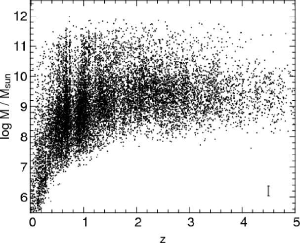
Figure 2: Stellar masses as a function of redshift. The typical error in mass is indicated in the lower right-hand corner.

In Fig. 2 we show the distribution of all galaxies in the mass versus redshift plane. We found five galaxies at high redshifts $z>4$ with masses $\log\,M/M_{\sun}>11.5$. The presence of such high–mass objects less than 2 Gyr after the big bang is still controversial (see, for example, Dunlop et al. 2007, and references therein). However, a closer analysis reveals that they are more likely to be heavily dust enshrouded galaxies at intermediate redshifts. While keeping the original upper limit in $A_{\mathrm{V}}$ for the remaining sample, to account for the degeneracy in age and extinction as explained above, we extended the parameter space by allowing a larger maximal dust extinction of $A_{\mathrm{V}}=4$ magnitudes for these five galaxies. Refitting the objects’ redshifts with our full template library leads to much smaller redshifts $z\approx 2$ and typical masses about $\log\,M/M_{\sun}\approx 10.5$ for four of the galaxies. With this reanalysis, the fit quality of our best matching SED template increases significantly and becomes comparable to the mean for these four objects. The fifth galaxy remains at high $z$ primarily because of an unexpected low $\mathrm{K_{S}}$–band luminosity, which may be a result of incorrect photometry. Nevertheless, we want to emphasize that it is not possible to draw an unambiguous conclusion about the nature of these objects on the basis of currently available data. This uncertainty reflects the general character of samples with mainly photometric redshifts. While they can provide accurate data within a statistical analysis, for a dedicated study of rare object properties additional information is still required. To restrict our sample to a uniform parameter space, we excluded the five questionable galaxies from our analysis in Sect. 4.

4 The role of Spitzer

To study the impact of Spitzer/IRAC data on our analysis, we considered only those galaxies with errors in mass from the fitting process $\sigma_{\mathrm{log\,M}}<0.2$ ($\approx 13\,000$). With this restriction, about half of the objects were detected in at least three IRAC channels. However, even if a source has not been identified in a specific filter, an upper limit in flux was included into the analysis, which provides a valuable additional constraint and in general affects the derived stellar mass. For this sample we repeated the calculation of stellar masses as described in Sect. 3 but reduced photometric information to the filters $\mathrm{U_{38}}$, B, V, i, z, J, H and $\mathrm{K_{S}}$ only, i.e. excluded the four IRAC channels. This subset of our data represents a multi–band catalog with wavelength coverage from about 3500 Å to $23\,000$ Å, which was typically available to study the high redshift universe before facilities such as the Spitzer space telescope became operational. We were then able to study the influence of additional infrared photometry by comparing the properties of the best–fitting models directly.

We found stellar masses to be overestimated without Spitzer data on average. The mean deviation between the masses calculated with all filters up to IRAC channel 4 ($M_{\mathrm{U-4}}$) and those with limited photometry ($M_{\mathrm{U-K}}$) of the whole sample is $\log\,M_{\mathrm{U-4}}/M_{\mathrm{U-K}}=-0.18\leavevmode\nobreak\ \mathrm{dex}$ with a r.m.s. of 0.41. As shown in Fig. 3, this trend is relatively independent of mass itself, but has a strong dependency on redshift. Whilst the mean deviation up to a redshift of $z\approx 2$ is only moderate ($|\log\,M_{\mathrm{U-4}}/M_{\mathrm{U-K}}|<0.2\leavevmode\nobreak\ \mathrm{dex}$) and comparable to the typical error in mass, the difference reaches a maximum of $|\log\,M_{\mathrm{U-4}}/M_{\mathrm{U-K}}|\approx 0.5\leavevmode\nobreak\ \mathrm{dex}$ at $z\approx 3.5$. This corresponds to an overestimation of mass of more than a factor of three on average, whereas the scatter for individual sources is large in general, as indicated by the r.m.s. of the distribution. Therefore we can confirm the conjecture made by Fontana et al. (2006), who did the same analysis on the $\mathrm{K_{S}}$–selected subsample with about 3000 galaxies, although we found the effect of Spitzer/IRAC data to be somewhat more pronounced. At higher redshifts the difference in mass decreases again. We can therefore conclude directly that without further data points the extrapolation of object luminosities to longer wavelengths is not straight forward and induces systematic deviations. This result has been derived for a specific set of template SEDs with solar metallicity, a Calzetti extinction law, Salpeter IMF, and for fixed photometric redshifts. Although other choices of model parameters may result in different absolute values for stellar masses, we expect the detection of a systematic trend to be comparatively robust, as it depends on a relative deviation. This statement is supported by the results of Fontana et al. (2006) who found a similar trend despite using a different model template library and SED fitting procedure.

Figure 3: This figure shows the difference in masses calculated under the inclusion of the Spitzer bands ($M_{\mathrm{U-4}}$) and with restricted photometry ($M_{\mathrm{U-K}}$) as a function of redshift. Averaged over all redshifts, the dependency on stellar mass itself is also indicated (inset). Mean values (solid lines) and r.m.s. of the data–points (dashed lines) are shown.

Figure 4: Ratio of inferred absolute $\mathrm{K_{S}}$–band luminosities (upper panel) and shift in corresponding mass–to–light ratios in solar units (lower panel) as a function of redshift. The mean values (solid lines) and the r.m.s. of the data–points (dashed lines) are shown.

The immediate reasons for the deviation can be seen in Fig. 4, where shifts in both the underlying $\mathrm{K_{S}}$–band luminosities and the mass–to–light ratios are evident. For a robust calculation of stellar masses with the aid of infrared luminosities, a good knowledge of the slope of the spectra beyond the $4000$ Å break is mandatory. Whereas the brightness of an old massive galaxy decreases slowly in this wavelength range, a young low–mass object has a steep spectrum and the decline is much stronger. To distinguish between early and late type galaxies solely on the basis of the blue part of their spectra is difficult, because the possible presence of a starburst can alter a galaxy’s UV luminosity substantially. Furthermore, uncertainties in extinction strongly affect this wavelength range, which makes it even more difficult to reveal the fundamental properties of the underlying SED. Therefore several data points longward of $4000$ Å are required for a reliable estimation of stellar masses. However, at a redshift of $z=2.5$ the 4000 Å break lies at $14\,000$ Å, i.e. it has already passed the J filter, so the calculation is resting upon H and $\mathrm{K_{S}}$–band photometry predominantly, as the slope of the rest–frame optical/near–infrared part of a galaxy’s spectrum is characterized by the $\mathrm{H}-\mathrm{K_{S}}$ color only. At a redshift of $z\approx 3.5$, where the deviation is largest, the spectrum longward of the $4000$ Å break in rest–frame is covered solely by the $\mathrm{K_{S}}$–filter and is therefore insufficiently sampled. In general, photometry becomes increasingly uncertain at higher redshifts when objects fade, so the constraints on the slope weaken further. At this redshift, the systematic deviation in masses due to the inclusion of Spitzer data starts to dominate over possible intrinsic errors. This effect can be traced back to the assignment of model SEDs that are too old with too high an absolute infrared luminosity. A decrease in stellar mass is therefore often associated with attributing a younger model SED, i.e. there is a correlation between shift in masses and ages, as can be seen in Fig. 5. Since extinction influences the shape of the spectrum in a similar way to age, the degeneracy in the two quantities reduces the correlation. We show the change of the best fitting model SED for several galaxies in the appendix.

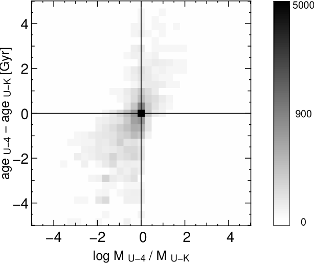
Figure 5: Correlation between the shift in masses (x–axis) and that in ages (y–axis) after inclusion of Spitzer photometry. The frequency of a specific combination is indicated by the color in nonlinear scaling. The correlation coefficient of the two quantities is $r=0.6$.

The reasons for decreasing differences in stellar masses for even higher redshifts beyond $z=3.5$ are twofold. First, the maximal age of a possible fit model is restricted by the age of the universe at that redshift, which acts as an upper limit. Therefore, the fit models are forced to be younger and a large decline in age with a lower resulting mass is therefore not likely. Secondly, at these extreme redshifts sources are very faint and an increasing fraction of our sample is hardly detected in the shallower J, H, and $\mathrm{K_{S}}$–band data. In this case, the calculation of masses without Spitzer data is mainly based on the V, i and z photometry (as galaxies are U and B–filter dropouts) and it turns out that very young low–mass model SEDs were assigned. With the inclusion of Spitzer bands the masses for this type of objects tend to increase, and the average difference of the whole sample gets smaller. We want to mention here that whereas the former effect is universal, the latter is a property of our specific catalog and may be less pronounced in other surveys.

In the next step we examined the influence of single Spitzer filters on the resulting stellar mass estimates. We repeated our calculations after adding the four Spitzer/IRAC bands to the analysis one by one. The outcome is illustrated in Fig. 6 where we show deviations in mass in relation to those calculated with full photometric information. Only one further data point at $3.6\leavevmode\nobreak\ \mu m$ can reduce the remaining shift in masses to less than $|\log\,M_{\mathrm{U-4}}/M_{\mathrm{U-1}}|\leq 0.25\leavevmode\nobreak\ \mathrm{dex}$ over the full redshift–range. After additionally taking into account Spitzer channel 2 at $4.5\leavevmode\nobreak\ \mu m$, the systematic deviation shrinks to $|\log\,M_{\mathrm{U-4}}/M_{\mathrm{U-2}}|\leq 0.1\leavevmode\nobreak\ \mathrm{dex}$ and thus becomes comparable to possible intrinsic errors attributed to the method used to derive stellar masses. Similarly, it is possible to reduce the deviation including just Spitzer channels 3 and 4 in the calculation. Although the remaining difference is at most $|\log\,M_{\mathrm{U-4}}/M_{\mathrm{U-K+3-4}}|\leq 0.24\leavevmode\nobreak\ \mathrm{dex}$ and therefore larger than in the case discussed above, and taking into account lower quality data, providing upper limits in flux can often significantly improve the result. Despite reduced mean deviations, the change in mass for single objects can still be large.

Figure 6: Deviation in mass as a function of redshift after including Spitzer filters one by one. Starting from masses calculated without Spitzer photometry (upper left panel, same as Fig. 3), the remaining deviation is shown for calculations based on photometry including Spitzer/IRAC data (up to channel 1, upper right; to channel 2, lower left; to channel 3, lower right). Mean values (solid lines) and the r.m.s. of the data–points (dashed lines) are plotted.

5 The stellar mass function

Because we found systematic shifts in calculated stellar masses, we wanted to examine the effects on resulting quantities such as the stellar mass function, i.e. the number of objects per comoving volume and mass interval. To do so, we subdivided our catalog into seven redshift bins from $z=0.25$ to $z=5$. Using this relatively coarse grid we still work with 380 objects in the highest $z$–bin and ensure that our results are based on statistically meaningful samples. Within each interval we calculated stellar mass functions after correcting our data points for incompleteness due to the flux–limited object selection utilising the $V/V_{\mathrm{max}}$–formalism of Schmidt (1968). In this context it is important to point out that we do not achieve a well defined completeness limit in stellar mass, as even for a sharp underlying flux limit, the dynamic range of mass–to–light–ratios results in a wide distribution in mass. Therefore the largest $M/L$–ratio at a certain redshift determines the limit in mass below which incompleteness starts to play a role. To quantify this effect we followed two different approaches. First, motivated by a more theoretical point of view, we studied the evolution of a passive evolving galaxy with subsolar metallicity and zero extinction formed at a redshift of $z=10$ in a single burst. By assuming an underlying flux limit of $\mathrm{z_{lim}}=26.0$ magnitudes we computed the corresponding stellar mass as a more conservative estimate for the completeness limit of the catalog. We found that galaxies with masses down to $M\mathrm{{}_{lim}}\approx 3\cdot 10^{9}\leavevmode\nobreak\ M_{\sun}$ can be detected at $z=1$. The value is increasing to $M\mathrm{{}_{lim}}\approx 3\cdot 10^{10}\leavevmode\nobreak\ M_{\sun}$ at $z=2.5$ where those objects would be detected in the shallower $\mathrm{K_{S}}$–band with an average flux limit of $\mathrm{K_{S\;lim}}=23.8$ magnitudes. This limit in mass is also obtained for old but moderately star–forming systems with extinctions around $A_{V}\approx 1$. In the second approach, which is motivated by the data actually available, we studied the evolution of the mass–to–light ratios of the catalog and calculated the 95 % quantile in $M/L_{z}$ as a function of redshift e.g. the limit below which 95 % of the $M/L_{z}$ ratios of our sample are located. Assuming a sharp flux limit such as adopted above, we computed the corresponding stellar mass as an estimate for completeness. For a redshift of $z=1$ we found this value to be $M\mathrm{{}_{lim}}\approx 2\cdot 10^{9}\leavevmode\nobreak\ M_{\sun}$ increasing to $M\mathrm{{}_{lim}}\approx 9\cdot 10^{9}\leavevmode\nobreak\ M_{\sun}$ at $z=2.5$. Although this more aggressive method results in a lower mass limit, it should be clear that a significant fraction of heavily dust enshrouded galaxies with large $M/L$–ratios may stay undetected at intermediate $z$, while a reliable detection of typical more massive active galaxies with low to intermediate extinctions should be possible up to high redshifts. As the two methods result in different completeness limits we performed the calculations in this section for both values independently.

To estimate the errors of the stellar mass function we used 1000 realisations of randomly drawn catalogs for which we have considered errors in computed redshifts, calculated $M/L_{\mathrm{K}}$–ratios and a general uncertainty in photometry. Finally, to cope with incompleteness at lower masses, in view of our subsequent analysis, we fitted our datapoints from the massive end down to the completeness limit with an analytical expression suggested by Schechter (1976) of the form:

$$\psi(M;\phi^{*},M^{*},\alpha)=log(10)\cdot\phi^{*}\cdot\left[10^{(M-M^{*})}\right]^{(1+\alpha)}\cdot exp\left[-10^{(M-M^{*})}\right]$$

In this formula the number density $\psi(M)$ is parameterized via a scale factor $\phi^{*}$, a typical mass $10^{M^{*}}M_{\sun}$ and a slope–parameter $\alpha$. First we computed the values of the fit parameters through an $\chi^{2}$–analysis in the redshift bins up to $z=4$ independently. We excluded the highest redshift interval at $4\leq z<5.01$ from the procedure, as we found the Schechter function to be insufficiently constrained due to the increasing mass limit. However, a robust estimation of the parameters is difficult as they are highly degenerated in the expression used. To deal with this problem we decided to fix the slope–parameter at its error–weighted mean value, as we found no clear evidence for an evolution with redshift as shown in the left–hand panel of Fig. 7. We also adopted this procedure because an undersampling of low mass objects in the catalog may affect the determination of the slope at higher redshifts in a systematic manner. With this constant value of $\alpha$ we repeated our calculation of the two remaining parameters $M^{*}$ and $\phi^{*}$ in every $z$–bin; for both completeness limits the result is plotted in Fig. 7 and listed in Table 1. A relatively uniform decrease in $\phi^{*}$ with redshift is clearly evident, which reflects the fact of a general decline in the number of detected objects in place. In contrast to the evident decrease of $\phi^{*}$, it is hard to say whether there is a hint at a mass dependent evolution of the number density, which would manifest itself as a shift in the parameter $M^{*}$. Although this trend would be expected by the downsizing scenario for galaxy evolution, where massive galaxies tend to form earlier than their low–mass counterparts, a slight increase in the typical mass with redshift followed by a decrease as indicated in the plot may also be the result of large–scale structure within the observed field.

The Schechter functions can be seen in Fig. 8, where we show the fit to the data with respect to the local stellar mass function of Cole et al. (2001) with the parameters $M^{*}$ = 11.16, $\phi^{*}$ = 0.0031 and $\alpha$ = -1.18. For comparison we also plot the mass function of Fontana et al. (2006), as derived from the $\mathrm{K_{S}}$–selected subsample of the GOODS–MUSIC catalog in slightly varied redshift bins up to $z\leq 4$. Besides a tendency to a smaller number of high mass objects, the datasets show a general agreement. The discrepancy at the high mass end turns out to be robust. Although results in this region rely on only a few galaxies, the error in mass is small for most of them. We discuss possible reasons for the deviations in detail in the next section. We also display the result of Drory et al. (2005) calculated from the FORS Deep Field (FDF) and a subarea of the GOODS–S (hereafter GSD) in the same redshift intervals without additional Spitzer infrared data. While the GSD data can be reproduced well up to intermediate redshifts, the analysis of the FDF sample tends to result in larger values for stellar mass function. At high redshifts, $z>3$, deviations are clearly visible for both the FDF and GSD datasets. They can be attributed to distinct effects; in addition to a shift in the mass scale as a result of the influence of Spitzer photometry, the total number of objects in the highest redshift intervals derived from an integral over the mass function is larger. Performing a Kolmogorov–Smirnov test on the redshift distributions of the FDF galaxies and the GOODS–MUSIC catalog used in this work, we can clearly reject the hypothesis that the two samples are drawn from the identical parent distribution at a 1 % level. However, both effects can have the same origin since the calculation of photometric redshifts becomes less reliable at high redshifts if the spectra are insufficiently constrained in the rest–frame optical, especially as spectroscopic redshifts used for comparison become very rare and are restricted to the most luminous objects.

Table 1: Schechter parameters of stellar mass functions as derived using the mass limits from a $M/L$–ratio analysis (upper section) and a passively evolving scenario (lower section, see text).

redshift interval	$M^{*}$	$\sigma_{M^{*}}$	$\phi^{*}\cdot 10^{4}$	$\sigma_{\phi^{*}}\cdot 10^{4}$	$\alpha$	$\sigma_{\alpha}$
$0.25\leq z<0.75$	11.51	0.06	8.43	0.60	-1.358	0.023
$0.75\leq z<1.25$	11.58	0.07	4.41	0.35	-1.358	0.023
$1.25\leq z<1.75$	11.59	0.07	3.20	0.31	-1.358	0.023
$1.75\leq z<2.25$	11.51	0.07	2.82	0.28	-1.358	0.023
$2.25\leq z<3.01$	11.34	0.06	2.66	0.24	-1.358	0.023
$3.01\leq z<4.01$	11.34	0.10	1.17	0.15	-1.358	0.023
$0.25\leq z<0.75$	11.50	0.06	8.77	0.62	-1.352	0.023
$0.75\leq z<1.25$	11.57	0.07	4.57	0.36	-1.352	0.023
$1.25\leq z<1.75$	11.58	0.07	3.29	0.32	-1.352	0.023
$1.75\leq z<2.25$	11.54	0.08	2.56	0.34	-1.352	0.023
$2.25\leq z<3.01$	11.48	0.08	1.89	0.28	-1.352	0.023
$3.01\leq z<4.01$	11.51	0.14	0.75	0.24	-1.352	0.023

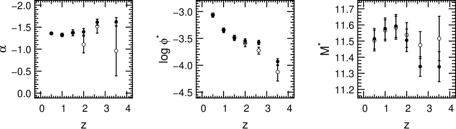
Figure 7: Evolution of Schechter parameters of the stellar mass function with redshift, showing the slope–parameter (left panel) as derived from an independent fit in each redshift interval. The remaining parameters $\phi^{*}$ (center) and $M^{*}$ (right panel) were recalculated using a fixed value for $\alpha$. They are interdependent in that a shift in $M^{*}$ to higher values, for example, would result in a smaller value of $\phi^{*}$. The results using mass limits from a $M/L$–ratio analysis (filled circles) and a passively evolving scenario (open circles, see text) are plotted.

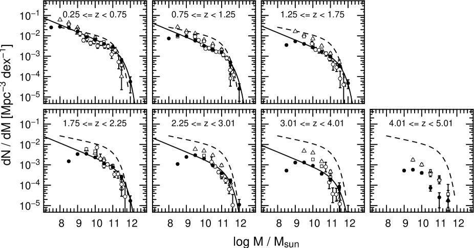
Figure 8: Evolution of stellar mass function with redshift, showing data points computed using the $V/V_{\mathrm{max}}$–formalism in seven different redshift intervals (filled circles) and, for $z\leq 4$, the best fitting Schechter functions utilizing mass limits from a $M/L$–ratio analysis (solid line, see text). For comparison we also plot the result of Drory et al. 2005 (open triangles FDF, open squares GSD) derived without additional Spitzer infrared data and the result of Fontana et al. (2006), calculated within slightly different redshift bins up to $z\leq 4$ (open circles), and the local Schechter function of Cole et al. (2001) (dashed line).

6 The stellar mass density

We are now able to compute stellar mass densities, i.e. the mass in stars and remnants per comoving volume at a specific redshift, on the basis of our results from Sect. 5. For this calculation we divided our stellar mass functions in each redshift bin into two mass intervals at the threshold values of the two completeness limits considered here. Above the limit, where data points and Schechter function fall together, we summed the stellar masses of our objects directly. In contrast to this procedure, we integrated the Schechter function in the low–mass range down to zero to take account of the fact that our catalog suffers from incompleteness here. The completion to lower masses contributes about 13 % (43 %) to the final mass density at the redshift interval $3.01\leq z<4.01$ using the mass limits derived from a $M/L$–ratio analysis (passive evolution scenario). In the highest redshift bin we summed stellar masses directly, not correcting for completeness. Although we certainly underestimate the resulting outcome for stellar mass density, a comparison to the values published by Drory et al. (2005) is still possible as the results were calculated without corrections there. In order to check our results for robustness, we dropped our assumption of a constant slope parameter $\alpha$ and recalculated stellar mass densities, but did not find appreciable deviations. To assign errors to the resulting data points we again used Monte Carlo simulations, and additionally considered uncertainties in the Schechter–parameters that affect the contribution of the integral over the low mass range only. However, a more careful analysis reveals that resulting errors may not include all sources of uncertainty. For example, cosmic variance can alter our result on a 20 % level when estimating the expected uncertainty in number density of observed objects (Somerville et al. 2004), although we were able to draw on a relatively large survey area of about 140 $\mathrm{arcmin^{2}}$ for our calculations. Another source of uncertainty is the proper treatment of stars in the post–AGB phase and their influence on stellar population synthesis models (see, for example, Maraston et al. 2006; Bruzual 2007; van der Wel et al. 2006). Furthermore, deviations from the assumed IMF can affect the outcome in a systematic way. In addition, it is important to point out that we can only give lower limits to the stellar mass densities, as we are not able to detect heavily dust enshrouded galaxies with large extinctions already at intermediate redshifts.

We list our results in Table 2, where we also compare the mass densities to the local value derived by Cole et al. (2001). It turns out that at a redshift of $\langle z\rangle=1$ at least 42 % of today’s stellar mass density is already in place. This fraction decreases to 22 % at $\langle z\rangle=2$ and about 6 % at $\langle z\rangle=3.5$. A comparison with values from literature derived on the basis of a photometric catalog without additional Spitzer/IRAC data is shown in Fig. 9. Whilst up to intermediate redshifts the stellar mass density is reproduced well (though with much smaller scatter because of a larger observed area), we find systematic deviations at high redshifts to lower densities, which one would expect from the properties of the stellar mass functions discussed in Sect. 5.

A comparison of this work with the result of Fontana et al. (2006), who used the $\mathrm{K_{S}}$–selected subsample of an almost identical catalog with about 3000 galaxies and integrated the Schechter function using smoothed parameters, shows systematically higher values for the stellar mass density. This trend is strengthening from $\log\,\rho_{\mathrm{this\;work}}/\rho_{\mathrm{Fontana\;et\;al.}}=0.11\leavevmode\nobreak\ \mathrm{dex}$ at a redshift of $\langle z\rangle=0.5$ to $0.31\leavevmode\nobreak\ \mathrm{dex}$ at $\langle z\rangle=3.5$. The discrepancy may have its origins in slightly different model grids used to infer mass–to–light–ratios, and in particular features of the utilized codes themselves. In contrast to the proceedings of Fontana et al. (2006), we restricted our template library to solar metallicity, but allowed for an independent burst component when fitting the object luminosities with model SEDs. As the difference in the inferred densities becomes more pronounced with redshift, it stands to reason that the derived masses of younger galaxies, in particular, are subject to systematic deviations. In general, they are affected by larger errors as the function of the mass–to–light–ratio steepens at low ages. Against the background of the discussed degeneracies in age, metallicity and extinction, differences in the underlying template models can affect calculated stellar masses more distinctly here. Similarly, an additional burst component can influence the derived stellar mass. If a galaxy reveals both a high UV luminosity due to a recent starburst and a large infrared luminosity i.e. substantial mass in an old population, a single component fit may not be able to reproduce the spectrum in the whole wavelength range simultaneously, as a young model is too faint in the infrared and an old model not bright enough in the blue. As a consequence, the inferred stellar mass can be lower (Wuyts et al. 2007). Therefore, splitting up the fit in burst and main component covers the range of mass–to–light–ratios in a more flexible fashion.

Table 2: Stellar mass densities, as derived using the mass limits from a $M/L$–ratio analysis (upper section) and a passively evolving scenario (lower section, see text). The redshift interval $4.01\leq z<5.01$ has not been corrected for completeness.

redshift interval	$log\,\rho(z)/[M_{\sun}Mpc^{-3}]$	$\sigma_{log\,\rho(z)}$	$\frac{\rho(z)}{\rho(z=0)}$
$0.25\leq z<0.75$	8.57	0.03	68.2 %
$0.75\leq z<1.25$	8.37	0.02	42.2 %
$1.25\leq z<1.75$	8.22	0.03	30.4 %
$1.75\leq z<2.25$	8.10	0.04	22.9 %
$2.25\leq z<3.01$	7.93	0.04	15.4 %
$3.01\leq z<4.01$	7.59	0.05	7.0 %
$4.01\leq z<5.01$	$>$ 6.90	0.08	1.4 %
$0.25\leq z<0.75$	8.57	0.03	68.1 %
$0.75\leq z<1.25$	8.36	0.02	42.2 %
$1.25\leq z<1.75$	8.22	0.03	30.4 %
$1.75\leq z<2.25$	8.08	0.06	21.9 %
$2.25\leq z<3.01$	7.89	0.06	14.1 %
$3.01\leq z<4.01$	7.61	0.25	7.4 %
$4.01\leq z<5.01$	$>$ 6.90	0.08	1.4 %

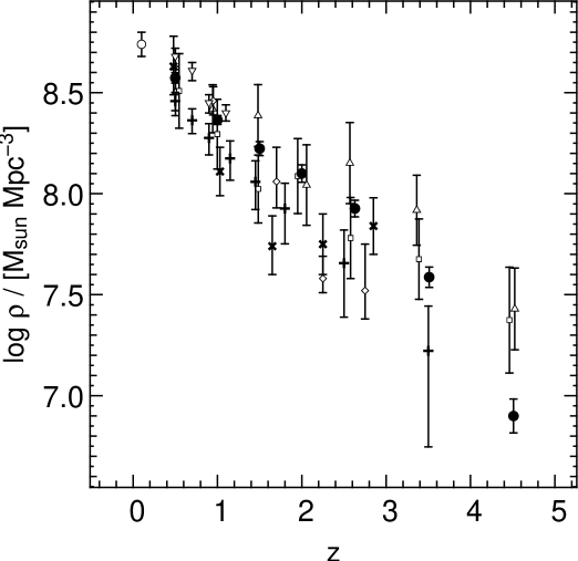
Figure 9: Stellar mass densities as a function of redshift. We compare stellar mass densities derived in the present work on an area of about 140 $\mathrm{arcmin^{2}}$ utilizing mass limits from a $M/L$–ratio analysis (filled circles, see text) to values from literature calculated without additional Spitzer/IRAC photometry. The results of Drory et al. 2005 (open triangles for FDF, 40 $\mathrm{arcmin^{2}}$; open squares for GSD, 50 $\mathrm{arcmin^{2}}$), Dickinson et al. 2003b (open diamonds, from HDF–N, 5 $\mathrm{arcmin^{2}}$), Fontana et al. 2003 (tilted crosses, from HDF–S, 5 $\mathrm{arcmin^{2}}$), Drory et al. 2004a (reversed triangles, from MUNICS survey, 0.28 $\mathrm{deg^{2}}$) and the local value (Cole et al. 2001, empty circle) are shown. We also plot the datapoints of Fontana et al. (2006) (upright crosses, GOODS–S, 140 $\mathrm{arcmin^{2}}$) as derived from the $\mathrm{K_{S}}$–selected subsample of the catalog including IRAC photometry by integrating the best fitting Schechter functions with smoothed parameters.

7 Summary

In this work we estimated the influence of newly available infrared data longward of the K–filter on stellar mass estimates. To do so we used the GOODS–MUSIC catalog published by Grazian et al. (2006), which combines photometric data in 10 filters from 0.35 to 2.3 $\mu m$ with observations from the IRAC instrument of the Spitzer space telescope at 3.6, 4.5, 5.8 and 8.0 $\mu m$. The catalog consists of 14 847 objects within an area of 143.2 $\mathrm{arcmin^{2}}$ detected either in the z or the $\mathrm{K_{S}}$–band. We computed stellar masses of this sample by fitting stellar population synthesis models (Bruzual & Charlot 2003) to the data and multiplying the k–corrected absolute $\mathrm{K_{S}}$–band luminosity with the $M/L_{\mathrm{K}}$–ratio of the best fitting model SED. To probe the influence of the IRAC data on the analysis we repeated the computation of stellar masses without Spitzer photometry, keeping the photometric redshifts fixed, and compared the outcome directly.

We found stellar masses to be overestimated on average, if further constraining infrared data from Spitzer were not included in the calculation. Whilst this trend is almost independent of mass itself, a closer analysis reveals a strong dependency on redshift. While up to $z\approx 2$ the systematic deviation in mass is only moderate ($|\log\,M_{\mathrm{U-4}}/M_{\mathrm{U-K}}|<0.2\leavevmode\nobreak\ \mathrm{dex}$) and comparable to the intrinsic uncertainty of the method adopted to estimate stellar masses, it increases strongly for higher redshifts and reaches a maximum of a factor of three at $z\approx 3.5$. The reason for this systematic shift can be traced back to insufficient constraints on the slope of the spectra redward of the 4000 Å break at high redshifts. It turns out that, on average, models that are too old, with excessively high absolute infrared luminosities and $M/L$–ratios were assigned to the data if Spitzer photometry is not included. Thus, a shift to lower stellar masses is likely to be correlated with a decreasing age of the best fitting model SED. The inclusion of one additional data–point longward of $3\leavevmode\nobreak\ \mu m$ can already reduce the remaining error in mass significantly.

In the next step we used our results to calculate stellar mass functions in different redshift intervals utilizing the $V/V_{\mathrm{max}}$–formalism of Schmidt (1968) to correct our sample partly for incompleteness. To assign errors we performed extensive Monte Carlo simulations where we considered uncertainties in the underlying $M/L_{\mathrm{K}}$–ratios, redshifts and a general error in photometry. Afterwards, the data points were fitted via three free parameters using the analytical expression suggested by Schechter (1976). We found a pronounced general decrease in numberdensity of all objects with redshift. Beyond that, it is hard to say whether there is also a mass dependent evolution. Although the change in computed Schechter parameter may support this position, the effect can be caused by large–scale structure as well.

Finally, we computed stellar mass densities as a function of redshift. We summed the mass of our objects within each redshift interval at the high mass end and integrated the Schechter function derived on the basis of our stellar mass functions to complete the result for lower masses. To estimate errors we again used Monte Carlo simulations, but we pointed out that further effects such as biases in stellar population synthesis models may be dominating sources of uncertainty. By comparing the outcome to the local value of Cole et al. (2001) we found at least 42 % of the stellar mass density to be already in place at $\langle z\rangle=1$. This value decreases to 23 % at $\langle z\rangle=2$ and about 7 % at $\langle z\rangle=3.5$. Therefore, up to intermediate redshifts our results are in good agreement with values taken from literature derived without additional Spitzer/IRAC data. However, at high redshifts a systematic deviation to lower densities is present as one would expect from the effect of Spitzer photometry on the calculation.

Appendix A Examples of SED–fits

We show some examples of a change in the best fitting model SED due to inclusion of Spitzer photometry. The shift in calculated stellar masses becomes manifest in a change of age, SFH and extinction (Figs. 10, 11) or the overall normalization (Fig. 12). In general, even a slight variation of the $\mathrm{K_{S}}$–band luminosity can change the derived stellar mass substantially if IRAC photometry is not taken into account. On the other hand, we occasionally found the slope of the spectra at longer wavelengths insufficiently constrained because of large photometric errors (Fig. 13).

Figure 10: Example of a change in the best fitting model SED (solid line) due to inclusion of Spitzer photometry. Upper panel: Without Spitzer/IRAC data the observed flux (filled circles) is fitted with a young starburst (dashed line) superimposed to a 1.5–Gyr–old main component with large extinction (dot–dashed line). Lower panel: After factoring in complementing infrared data, extinction decreases and the best fitting model SED becomes younger. The resulting stellar mass reduces from $\log\,M_{\mathrm{U-K}}/M_{\sun}=10.32\;\mathrm{dex}$ to $\log\,M_{\mathrm{U-4}}/M_{\sun}=9.69\;\mathrm{dex}$.

Figure 11: Same as Fig. 10. The change in the fit to photometric data where the extinction varies is shown. The resulting stellar mass reduces from $\log\,M_{\mathrm{U-K}}/M_{\sun}=10.07\;\mathrm{dex}$ to $\log\,M_{\mathrm{U-4}}/M_{\sun}=9.54\;\mathrm{dex}$.

Figure 12: Same as Fig. 10. The change in the fit to photometric data where the absolute normalisation changes distinctly is shown. The resulting stellar mass decreases from $\log\,M_{\mathrm{U-K}}/M_{\sun}=9.26\;\mathrm{dex}$ to $\log\,M_{\mathrm{U-4}}/M_{\sun}=8.52\;\mathrm{dex}$.

Figure 13: Same as Fig. 10. The figure shows an example of an insufficiently constrained optical– to near–infrared–luminosity due to large photometric errors. The resulting stellar mass decreases from $\log\,M_{\mathrm{U-K}}/M_{\sun}=9.45\;\mathrm{dex}$ to $\log\,M_{\mathrm{U-4}}/M_{\sun}=8.65\;\mathrm{dex}$.

References

- Bell et al. (2003) Bell, E. F., McIntosh, D. H., Katz, N., & Weinberg, M. D. 2003, ApJS, 149, 289
- Borch et al. (2006) Borch, A., Meisenheimer, K., Bell, E. F., et al. 2006, A&A, 453, 869
- Brinchmann & Ellis (2000) Brinchmann, J. & Ellis, R. S. 2000, ApJ, 536, L77
- Bruzual (2007) Bruzual, G. 2007, ArXiv Astrophysics e-prints
- Bruzual & Charlot (2003) Bruzual, G. & Charlot, S. 2003, MNRAS, 344, 1000
- Calzetti et al. (2000) Calzetti, D., Armus, L., Bohlin, R. C., et al. 2000, ApJ, 533, 682
- Cole et al. (2001) Cole, S., Norberg, P., Baugh, C. M., et al. 2001, MNRAS, 326, 255
- De Santis et al. (2006) De Santis, C., Grazian, A., & Fontana, A. 2006, Memorie della Societa Astronomica Italiana Supplement, 9, 454
- Dickinson et al. (2003a) Dickinson, M., Giavalisco, M., & The Goods Team. 2003a, in The Mass of Galaxies at Low and High Redshift, ed. R. Bender & A. Renzini, 324–+
- Dickinson et al. (2003b) Dickinson, M., Papovich, C., Ferguson, H. C., & Budavári, T. 2003b, ApJ, 587, 25
- Dopita et al. (2005) Dopita, M. A., Groves, B. A., Fischera, J., et al. 2005, ApJ, 619, 755
- Drory et al. (2004a) Drory, N., Bender, R., Feulner, G., et al. 2004a, ApJ, 608, 742
- Drory et al. (2004b) Drory, N., Bender, R., & Hopp, U. 2004b, ApJ, 616, L103
- Drory et al. (2001) Drory, N., Bender, R., Snigula, J., et al. 2001, ApJ, 562, L111
- Drory et al. (2005) Drory, N., Salvato, M., Gabasch, A., et al. 2005, ApJ, 619, L131
- Dunlop et al. (2007) Dunlop, J. S., Cirasuolo, M., & McLure, R. J. 2007, MNRAS, 376, 1054
- Fontana et al. (2003) Fontana, A., Donnarumma, I., Vanzella, E., et al. 2003, ApJ, 594, L9
- Fontana et al. (2004) Fontana, A., Pozzetti, L., Donnarumma, I., et al. 2004, A&A, 424, 23
- Fontana et al. (2006) Fontana, A., Salimbeni, S., Grazian, A., et al. 2006, A&A, 459, 745
- Grazian et al. (2006) Grazian, A., Fontana, A., de Santis, C., et al. 2006, A&A, 449, 951
- Maraston et al. (2006) Maraston, C., Daddi, E., Renzini, A., et al. 2006, ApJ, 652, 85
- Rudnick et al. (2003) Rudnick, G., Rix, H.-W., Franx, M., et al. 2003, ApJ, 599, 847
- Schechter (1976) Schechter, P. 1976, ApJ, 203, 297
- Schmidt (1968) Schmidt, M. 1968, ApJ, 151, 393
- Somerville et al. (2004) Somerville, R. S., Lee, K., Ferguson, H. C., et al. 2004, ApJ, 600, 171
- van der Wel et al. (2006) van der Wel, A., Franx, M., Wuyts, S., et al. 2006, ApJ, 652, 97
- Werner et al. (2004) Werner, M. W., Roellig, T. L., Low, F. J., et al. 2004, ApJS, 154, 1
- Wuyts et al. (2007) Wuyts, S., Labbé, I., Franx, M., et al. 2007, ApJ, 655, 51