Dynamics of Vortex Formation in Merging Bose-Einstein Condensate Fragments

Abstract

We study the formation of vortices in a Bose-Einstein condensate (BEC) that has been prepared by allowing isolated and independent condensed fragments to merge together. We focus on the experimental setup of Scherer et al. [Phys. Rev. Lett. 98, 110402 (2007)], where three BECs are created in a magnetic trap that is segmented into three regions by a repulsive optical potential; the BECs merge together as the optical potential is removed. First, we study the two-dimensional case, in particular we examine the effects of the relative phases of the different fragments and the removal rate of the optical potential on the vortex formation. We find that many vortices are created by instant removal of the optical potential regardless of relative phases, and that fewer vortices are created if the intensity of the optical potential is gradually ramped down and the condensed fragments gradually merge. In all cases, self-annihilation of vortices of opposite charge is observed. We also find that for sufficiently long barrier ramp times, the initial relative phases between the fragments leave a clear imprint on the resulting topological configuration. Finally, we study the three-dimensional system and the formation of vortex lines and vortex rings due to the merger of the BEC fragments; our results illustrate how the relevant vorticity is manifested for appropriate phase differences, as well as how it may be masked by the planar projections observed experimentally.

I Introduction.

The formation, stability and dynamics of vortex-like structures has been a long-standing theme of interest in many areas of physics, including classical fluid mechanics batchelor , superfluidity and superconductivity Donnelly ; Tilley ; zurek , and cosmology kibble . Moreover, in the past decade, there has been a tremendous growth of excitement in this topic in the branches of atomic and optical physics. This has been propelled by considerable experimental and theoretical advances in the fields of nonlinear optics desyatnikov and Bose-Einstein condensates (BECs) in dilute alkali vapors fetter ; us (see also Ref. pismen ).

Focusing more specifically on the rapidly growing area of BECs review , one can recognize that the study of vortices has been central to the relevant literature. In particular, as concerns the experimental efforts, the original observations of single cornell1 ; Holland and multiple vortices dalib1 was soon followed by the realization of robust lattices of large numbers of vortices kett1 . Subsequent studies turned to higher-charged structures such as vortices of topological charge $S=2$ and even $S=4$ kett2 and illustrating dynamical instability of these topological objects kett3 . On the other hand, the abundance of experimental results has stirred an intense theoretical interest in the conditions under which such vortices and vortex lattices would be robust and experimentally observable. Most often, vortex existence and stability issues were examined in the framework of the standard parabolic confining potential (typically produced by magnetic traps). In that framework, and in the two-dimensional (2D) case, vortices of charge $S=1$ were found to be stable, while vortices of higher charge ($S=2,3$) were shown to be potentially unstable pu (depending on the atom numbers). Later, similar results were found for vortices of $S=4$ kawa , while the availability of more substantial computational resources has more recently led to similar conclusions in the fully three-dimensional (3D) case jukka1 ; jukka2 . The studies of Refs. motto and ueda examined the various scenarios of break-up of higher-charge vortices during dynamical evolution simulations for repulsive and attractive interactions respectively. Furthermore, Ref. carr considered such vortices riding on the background of not just the ground state, but also of higher, ring-like, excited states of the system. It should also be mentioned that these advancements have motivated the development of mathematically rigorous tools in order to study the spectrum of such vortex modes. Such methods involve the use of the Evans function kollar , or the use of the index theorem evaluating the number of potentially unstable eigendirections todd .

Although the existence and stability of fundamental and higher charge vortices has been examined extensively as indicated above, the formation of such vortex structures is far less studied. In particular, while seminal interference experiments (demonstrating that BECs are coherent matter waves) were reported as early as a decade ago science , the role of interference between BECs in vortex generation was experimentally studied only recently bpa_prl . This work proposed and examined the formation of vortices resulting from the interference and controlled merging of three condensed fragments, where the fragments were essentially independent BECs separated by an optical potential barrier. Such a process has close ties to elements of topological defect formation in phase transitions, as proposed by Kibble kibble and Zurek zurek . Interestingly, the experimental work was almost concurrent with a theoretical study investigating a simpler elongated barrier separating two independent BECs ric ; in the latter setting, the interference forms a dark soliton whose bending and subsequent breakup due to the manifestation of the transverse modulational instability also result in vortices.

In the present work, we expand on these considerations and study in detail, by means of systematic numerical simulations, the formation of vortices in a setting closely matching the one of the experiment in Ref. bpa_prl . Our purpose is to get a deeper insight into this interference-induced vortex formation mechanism, investigating fundamental features, such as the number and lifetime of ensuing vortices. This is done upon studying in detail the parametric dependences influencing the relevant experimental observations. Specifically, we quantify the above mentioned features as functions of the elimination/ramping-down time of the optical barrier between the fragments, or the initial relative phases between the original independent fragments. Our investigation chiefly refers to a 2D setting, but we also illustrate how the results are generalized in the pertinent 3D case. Notice that our considerations are motivated not only by their direct bearing on the experiments of Ref. bpa_prl , but also by their relevance to studies of spontaneous symmetry breaking during phase transitions zurek ; kibble ; sanders .

Our presentation is structured as follows. In Sec. II, we briefly summarize the setup of our computational experiments. In Sec. III, we study the interference of three BEC fragments in the 2D and 3D setup; special attention is payed at the role of the relative phases between the different condensates, and the ramp-down time of the laser sheet barrier responsible for separating the three fragments. In Sec. IV, we briefly comment on the relation between numerical and experimental results. Finally, in Sec. V, we summarize our findings, present our conclusions, and discuss some possible extensions of this work.

II Setup

We consider a BEC at a temperature close to zero, where quantum or thermal fluctuations are negligible (note that finite temperature effects are briefly discussed at the end of Sec. III). This system can accurately be described by a mean-field theoretical model, namely the Gross-Pitaevskii equation (GPE) review :

$$i\hbar\frac{\partial\psi}{\partial t}=\left[-\frac{\hbar^{2}}{2m}\nabla^{2}+V({\bf r};t)+g|\psi|^{2}\right]\psi,$$ (1)

where $\psi=\psi({\bf r},t)$ is the condensate wavefunction (with $n({\bf r},t)\equiv|\psi({\bf r},t)|^{2}$ being the atomic density of the condensate), $m$ is the atomic mass, the coupling constant $g=4\pi\hbar^{2}a_{s}/m$ measures the strength of inter-atomic interactions and $a_{s}$ is the $s$-wave scattering length. The potential $V({\bf r};t)$ in the GPE is taken to be of the form,

$$V({\bf r};t)=V_{\rm MT}({\bf r})+\alpha(t)\,V_{\rm L}({\bf r}),$$ (2)

where the two components in the right-hand side of Eq. (2) are a harmonic magnetic trap, $V_{\rm MT}({\bf r})=\frac{1}{2}m(\omega_{x}^{2}x^{2}+\omega_{y}^{2}y^{2}+\omega_{z}^{2}z^{2})$, with trapping frequencies $\omega_{x}=\omega_{y}=2\pi\times 7.4$ Hz and $\omega_{z}=2\pi\times 14.1$ Hz, and the three-armed time-dependent optical barrier, $\alpha(t)V_{\rm L}({\bf r})$, used in the experiments of Ref. bpa_prl . This three-armed potential induces a separation of the ground state of the condensate into three different fragments (see top-left and top-center panels in Fig. 1 and Fig. 11(a)). Note that the function $\alpha(t)$ in Eq. (2) describes the ramping down of the optical barrier. The maximum initial barrier energy for the potential is taken to be $\alpha_{0}\equiv\alpha(0)=26\,k_{B}$ nK bpa_prl , where $k_{B}$ is Boltzmann’s constant.

In the numerical simulations, the ground state of the system is obtained by relaxation (imaginary time integration) initiated with the Thomas-Fermi (TF) approximation (see top-center panel in Fig. 1)

$$\psi({\bf r},0)=\sqrt{\max\{0,\mu-V({\bf r})\}}\times\phi({\bf r}),$$ (3)

where $\mu=8\,k_{B}$ nK bpa_prl is the chemical potential, and $\phi({\bf r})$ contains the chosen phase of the different wells separated into the three regions A, B and C depicted in the top-right panel of Fig. 1. Let us denote by $\phi_{1}$, $\phi_{2}$, and $\phi_{3}$ the initial phases in regions A, B and C, respectively. It is important to note that while in the experiments of Ref. bpa_prl the different fragments have uncorrelated (random) phases, in our numerical simulations we are able to control their initial phases and, more importantly, their relative phases. Our numerical experiments, emulating the experimental sequence of Ref. bpa_prl , are performed with the output of imaginary time relaxation used as initial condition for the full dynamics of Eq. (1). The bottom row of Fig. 1 depicts the evolution of the phase for the case $\phi_{k}=2\pi k/3$ during relaxation. As can be observed from the figure, the initial “seed” ($t=0$) starts with sharp phase boundaries around the localized fragments. As the relaxation procedure evolves, the phase boundaries become smoother and adjust to the boundaries for the top-right panel of the figure. The phase profile seems to settle after 10 ms of imaginary time relaxation. In our simulations, 50 ms of imaginary time relaxation was used to ensure proper convergence to the steady-state solution.

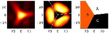
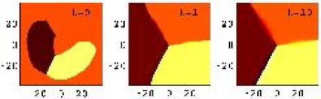
Figure 1: (Color online) Top-left: intensity profile of the optical potential responsible for segmenting the potential well into three local minima. Top-center: Thomas-Fermi approximation used as an initial condition for our relaxation method to obtain the ground state of the system. Top-right: regions A, B, and C with respective phases $\phi_{1}$, $\phi_{2}$, and $\phi_{3}$. The bottom row of panels depicts the evolution of the phase during our relaxation (imaginary time relaxation) towards the initial steady state with different phases for the fragments. This example shows the phase for the case $\phi_{k}=2\pi k/3$ at the times indicated. In all panels, the field of view is approximately 70 $\mu$m per side. The axis numbers indicate $x$ and $y$ coordinates relative to the center of the unsegmented harmonic trap.

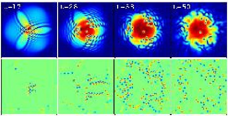
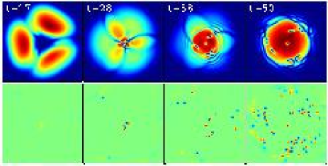
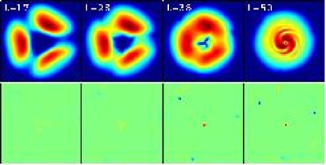
Figure 2: (Color online) Evolution of the 2D condensate density (respective top series of panels) and vorticity (respective bottom series of panels) for three different ramp-down times of the optical potential barriers. From top to bottom, the three sequences correspond to $t_{b}=0$ ms (first and second row), $t_{b}=25$ ms (third and fourth row), and $t_{b}=50$ ms (fifth and sixth row). The times are indicated in the panels in ms and the field of view is approximately 70 $\mu$m per side. For the initial conditions in all cases, the different condensed fragments have relative phases of $2\pi/3$, namely, $\phi_{k}=2\pi k/3$ ($k\in\{1,2,3\}$).

III Numerics.

III.1 Two-dimensional BECs.

For the 2D rendering of the experiment of Ref. bpa_prl , we restrict our system to the $(x,y)$ coordinates and we use the same chemical potential as in Ref. bpa_prl . First we explore the effect of the ramp-down time of the potential barrier on the formation of vortices through the merging of the different fragments of the condensate. For this purpose we use a linear ramp:

$$\alpha(t)=\max\left\{\frac{\alpha_{0}}{t_{b}}(t_{b}-t),\,0\right\},$$ (4)

where $\alpha_{0}\equiv\alpha(0)$ is the maximum barrier energy as defined above and $t_{b}$ is the ramping time (in ms) of the barrier; note that a similar ramp was used in the experiments of Ref. bpa_prl .

We monitor the formation of vortices, as well as the overall vorticity of the system, using various diagnostics. These are based on the corresponding fluid velocity of the superfluid given by Jackson:prl:98 ,

$${\mathbf{v}}_{s}=-\frac{i\hbar}{2m}\frac{\psi^{*}\nabla\psi-\psi\nabla\psi^{*}}{|\psi|^{2}},$$ (5)

where $(\cdot)^{*}$ stands for complex conjugation. The fluid vorticity is then defined as $\mbox{\boldmath$\omega$}=\nabla\times{\mathbf{v}}_{s}$. The results for the merger of the three BEC fragments with relative phases $\phi_{k}=2\pi k/3$, $k\in\{1,2,3\}$, for different merging times are depicted in Fig. 2. As can be seen from the figure, the number of vortex pairs nucleated by the merger is extremely sensitive to the ramping time $t_{b}$. Shorter ramping times give rise to an extremely rich vorticity pattern as the fragments merge [see, for example, the top two rows in Fig. 2 corresponding to the instantaneous ($t_{b}=0$) removal of the barrier], including the appearance of structures resembling vortex streets. However, for longer ramp times, i.e. slower ramping, just a handful of vortices are nucleated. In fact, for $t_{b}>100$ ms (results not shown here), the only vortex that is nucleated is the central one. It is evident that, independently of the ramping time, the central vortex is always formed for this pair of relative phases between the fragments. This vortex is the consequence of the intrinsic vorticity present in the initial condition where the three fragments have been phase imprinted with a total of a $2\pi$ phase gain about the condensate center.

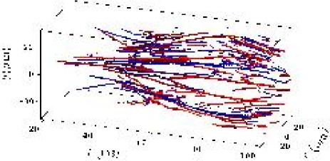
Figure 3: (Color online) Evolution of the vortex structures in the 2D condensate density for $t_{b}=25$ ms and $\phi_{k}=2\pi k/3$ (cf. middle rows in Fig. 2).

In Fig. 3 we present a spatio-temporal rendering of the vortex formation for the middle row example of Fig. 2 (i.e., phases given by $\phi_{k}=2\pi k/3$ and a ramp down time of $t_{b}=25$ ms). In the figure we depict a space-time contour plot of the vorticity where blue/red contours correspond to negatively/positively charged vortices, respectively. The figure clearly shows the formation of pairs of vortices with opposite charge, some of which self-annihilate at later times, while others oscillate together with the cloud: upon formation, they expand to the rims of the cloud and are subsequently reflected from its outskirts and contract anew, following the density profile oscillations resulting from the merging process.

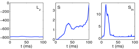
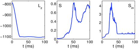
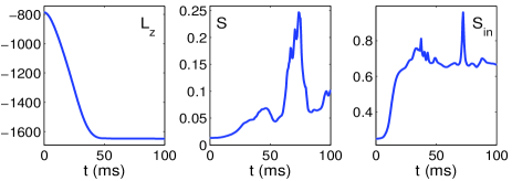
Figure 4: (Color online) Vorticity indicators for the cases presented in Fig. 2 (namely, $t_{b}=0$ ms, $t_{b}=25$ ms, and $t_{b}=50$ ms, from top to bottom) with $\phi_{k}=2\pi k/3$. The left panels correspond to the total angular momentum [Eq. (6)] normalized by $\hbar$, while the middle and right panels correspond to the total fluid velocity [Eq. (8)] for the whole cloud (middle) and the central portion (see text) of the cloud (right).

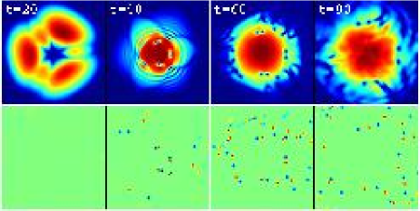
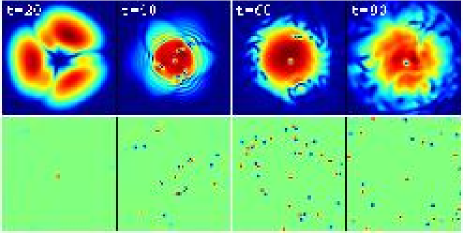
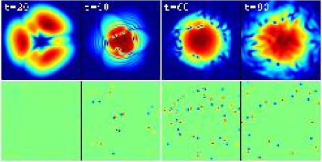
Figure 5: (Color online) Same as in Fig. 2 for three different relative phases and a ramp down of $t_{b}=25$ ms. The top two, middle two and bottom two series correspond, respectively, to: a) $\phi_{k}=0$, b) $\phi_{1}=0$, $\phi_{2}=2\pi/3$, and $\phi_{3}=4\pi/3$, and c) $\phi_{1}=0$, $\phi_{2}=\pi/3$, and $\phi_{3}=2\pi/3$.

In order to measure the vorticity generated during the merger of the condensate fragments at any given time, we compute the expectation value of the $z$-component of the angular momentum of the BEC

$$L_{z}=i\hbar\,\int\psi^{*}\,\partial_{\theta}\psi\,d{\bf r}\equiv\left(\psi,(\hat{\bf r}\times\hat{\bf p})_{z}\psi\right),$$ (6)

where $\hat{\bf r}$ and $\hat{\bf p}$ denote the corresponding position and momentum operators, the subscript $z$ indicates the component of the corresponding cross-product and $(\cdot,\cdot)$ indicates the complex inner product defined from $C\times C\rightarrow C$. Using Eq. (6) and Eq. (1), we can evaluate the time derivative of this expectation value:

$$\frac{dL_{z}}{dt}=\frac{\alpha(t)}{\hbar}\int|\psi|^{2}(\hat{\bf r}\times\hat{\bf p})_{z}V_{L}({\bf r})d{\bf r}.$$ (7)

In obtaining this result, we have assumed the isotropy of $V_{\rm MT}({\bf r})$ in the $(x,y)$ plane. This result also has some important consequences including the fact that during the ramp down of the optical barrier, we should not expect the angular momentum of the BEC to be conserved, while we should expect such a conservation to appear once $\alpha(t)=0$ or, more generally, when the full potential is azimuthally isotropic in the $(x,y)$ plane (cf. Figs. 4 and 6). In the left column of Fig. 4 we depict the $z$-component of the angular momentum. The middle column of the same figure shows a quantity that we refer to as total fluid velocity, defined as:

$$S=\frac{1}{V}\int|{\mathbf{v}}_{s}|\,d{\bf r},$$ (8)

where $V=\int d{\bf r}$ is the total volume of integration. Finally, the right column of Fig. 4 shows the same quantity, as defined in Eq. (8), but only for the central portion of the cloud. The central portion of the cloud was defined as a square, centered at the center of the magnetic trap, with a side equal to 10% of the integration domain. This area corresponds approximately to the void area between the three initial fragments (see top-center panel in Fig. 1).

The three diagnostics defined above are shown in Fig. 4 for the same cases presented in Fig. 2. It is interesting to note how the presence of a time-dependent component in the potential generates angular momentum in the system. As can be observed in the figure, the total angular momentum increases (in absolute value) through the duration of the barrier ramp-down and then settles to a constant value that is larger (in absolute value) for slower ramps. Also, it is worth noting that the initial value of the angular momentum is different from zero [$L_{z}(t=0)\approx-800$] due to the intrinsic vorticity carried by the out-of-phase fragments (see also discussion below). For our initial condition, most of the total angular momentum is seeded in the weak overlapping region between the fragments where the phase gradient is large. What we can observe about the second and third diagnostics by comparing (the second row of) Fig. 2 and Fig. 3 with (the second row of) Fig. 4 is roughly the following: the integrated (throughout the cloud) velocity appears to peak when the filamentation in the pattern of Fig. 3 is maximal, e.g., around times of 50 and 90 ms. On the other hand, the same diagnostic integrated within the central core of the cloud peaks substantially earlier when the vortices are formed through the collision of the fragments around the end time of the ramp (i.e., around 25 ms). Subsequently, and as the vortices are advected away from the core, the latter quantity decreases.

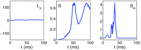
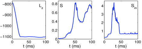
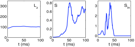
Figure 6: (Color online) Vorticity indicators for the cases depicted in Fig. 5 (the different panels are presented in the same manner as in Fig. 4).

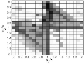
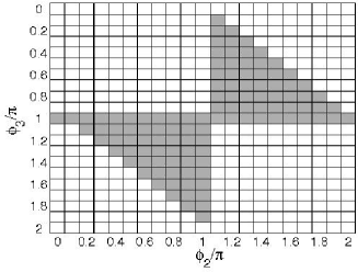
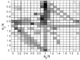
Figure 7: Phase diagram for vortex formation at the trap center region as a function of the relative phases of the merging fragments (where $\phi_{1}$ is assigned the value of 0). Top: Ramp down time of $t_{b}=0$ ms (i.e., instantaneous removal) of the barrier. The different shades of gray indicate the amount of vorticity contained in the central region after 100 ms. White, light gray, gray, black correspond, respectively, to 0, 1, 2, and 3 vortices. Middle: Same as above for a ramp down time of $t_{b}=50$ ms. This case only produces no vortices (white) or one vortex (gray). Bottom: difference between top and middle diagrams. This corresponds to the vortices formed by the collision of the fragments and not by the intrinsic vorticity of the initial configuration (which depends on the relative phases of the different fragments).

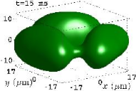
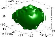
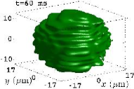
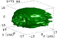
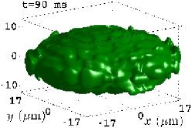
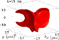
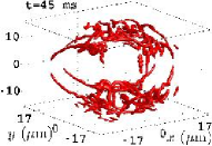
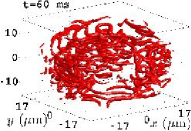
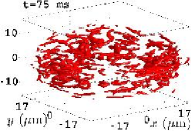
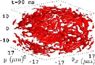
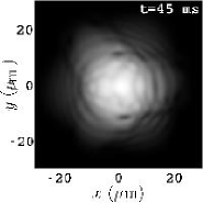
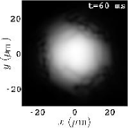
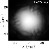
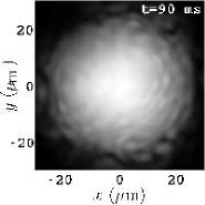
Figure 8: (Color online) Vortex formation by the merging of three-dimensional BECs. Top row: contour surfaces of constant atomic density. Middle row: contour surfaces of the corresponding absolute value of the vorticity. Bottom row: $z$-projection of the density distribution (i.e., column density along $z$) as it would be observed in the laboratory. The snapshots are taken at the indicated times (in ms) for an initial phase distribution corresponding to $\phi_{k}=0$ and a ramping down time of 25 ms. For the contour-surface images, the axis on the left side of each plot represents the vertical ($z$) direction, expressed in units of microns.

We now turn to the examination of the effect of the relative initial phases between the different fragments. As an example, we show in Fig. 5 the behavior of the cloud density and its vorticity for three different phase combinations for a fixed ramp-down time of $t_{b}=25$ ms. As can be noticed, the complexity of the vorticity field is similar for the three cases shown in the figure. However, the only phase combination of the ones shown here that produces a vortex at the center of the cloud corresponds to $\phi_{k}=2\pi k/3$, which can be understood by the intrinsic vorticity already present in the initial configuration (see explanation below). In Fig. 6 we depict the vorticity indicators for the three phase combinations of Fig. 5. As can be seen in the figure, the angular momentum $L_{z}$ for $\phi_{k}=0$ (top-left panel) and $\phi_{k}=\pi k/3$ (bottom-left panel) suffers almost no change since the initial configuration does not carry any intrinsic vorticity and thus, its interaction with the ramping down barrier does not produce angular momentum. However, for $\phi_{k}=2\pi k/3$ (middle-left panel), as explained before, the system does gain angular momentum during the barrier removal. The total fluid velocity indicators (middle and right columns in Fig. 6 behave similarly for the three phase combination with the notable difference that for the $\phi_{k}=2\pi k/3$ (middle-left panel) case, its final value is different from zero since the fragments produce a vortex at the center of the trap (due to the intrinsic vorticity carried by the initial condition).

In order to follow in more detail the formation of vortices in the central portion of the cloud as a function of the relative initial phases of the different fragments, we perform systematic simulations for a large set of relative initial phases. The results are presented in Fig. 7, where we show the existence of vortices as a function of $(\phi_{2},\phi_{3})$ for $\phi_{1}=0$. Darker shades correspond to the presence of more vortices. The top panel of Fig. 7 corresponds to an immediate release of the barrier (ramp down time of $t_{b}=0$ ms) where the presence of 0, 1, 2 or 3 vortices (white, light gray, gray, and black respectively) can be observed for different phase combinations. The middle panel depicts the same diagram, but for a ramping-down time of $t_{b}=50$ ms. It is clear that, for this relatively slow ramp down, the formation of a vortex in the central region is exclusively determined by the vorticity of the initial configuration. Namely, if any of the relative phases is larger than $\pi$, the initial configuration resembles more that of a discrete vortex (see Refs. panos and desyatnikov ; our for reviews). In particular, each fragment can be thought of a “unit” and the whole configuration corresponds to a discrete vortex with three units with a net vorticity different from zero. The middle panel of the figure clearly reveals that only within an arc of the second (and essentially symmetrically of the fourth) quadrant of the plane of the phases $(\phi_{2}-\pi,\phi_{3}-\pi)$, a single vortex will form at the center of the configuration. It is interesting that discrete vortex-like configurations consisting of three fragments have been considered in the context of nonlinear optics in Ref. sukh and even in genuinely discrete systems as, e.g., in Ref. kouk . In the bottom panel of Fig. 7 we depict the difference between the top and middle panels to show the amount of vortices that are created exclusively by the fragment collision and not by the intrinsic vorticity of the initial configuration. It is important to mention that some of the vortices counted in the top panel come from vortices that are created outside the central region but that migrate towards the center as time progresses.

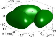
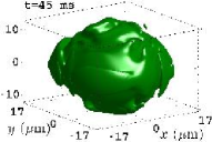
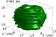
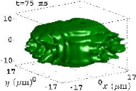
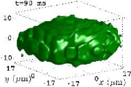
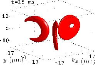
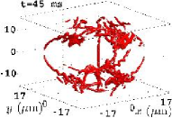
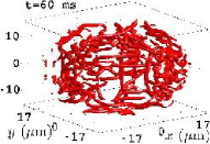
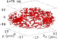
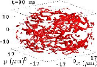
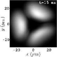
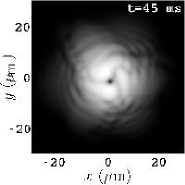
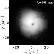
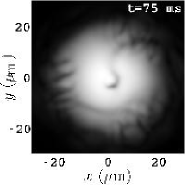
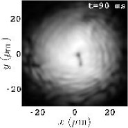
Figure 9: (Color online) Same as in Fig. 8 for an initial phase distribution corresponding to $\phi_{k}=k2\pi/3$.

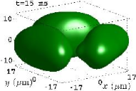
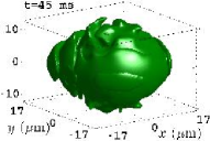
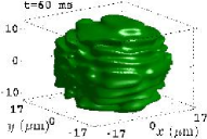
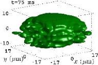
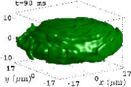
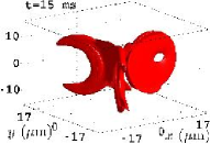
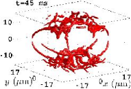
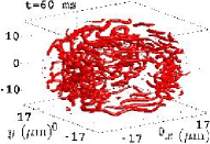
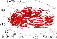
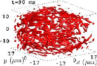
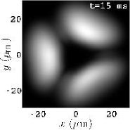
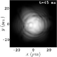
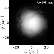
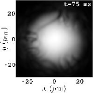
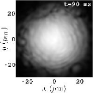
Figure 10: (Color online) Same as in Fig. 8 for an initial phase distribution corresponding to $\phi_{k}=k\pi/3$.

III.2 Three-dimensional BECs.

As shown in the previous section, the 2D setting lends itself to a more detailed examination of important features such as the parametric dependence on the ramping time and the relative phases of the fragments. Nevertheless, it is important to also consider some of the delicate points particular to the 3D nature of the experiments and the observable quantities available within the experimental images. For this reason, we now focus on the 3D setting, presenting results of the simulations relevant to the experiment of Ref. bpa_prl . The setup is the same as in the previous section but we now use the full 3D space with the same chemical potential as before. Typical results are shown in Figs. 8–10 for a ramping down time of the potential barrier of 25 ms. Figure 8 corresponds to the case of equal initial phases $\phi_{k}=0$, while Fig. 9 pertains to initial phases $\phi_{k}=2\pi k/3$, and Fig. 10 to phases $\phi_{k}=\pi k/3$. The figures depict contour plots of the density (top rows) and vorticity (middle rows), as well as a $z$-projection of the density (bottom rows) as it would be observed in the laboratory. The vortex structure is considerably more complex in the 3D scenario because the vorticity does not show up as straight vortex lines but rather as a complex web of vortex filaments in various directions. As in the 2D case, there is the formation of a vertical vortex line at the center of the cloud (cf. second row in Fig. 9) for the appropriate relative phases of the different fragments of the condensate with the same conditions as before. Nonetheless, in the 3D case, the central vortex line is prone to bending as can be clearly seen in the later stages of the dynamical evolution presented in the second row of Fig. 9. In fact, the vortex bending is even clearly visible in the $z$-projection (see third row of Fig. 9). These 3D numerical experiments are quite revealing in that the laboratory experiments can only show projections of the density and thus missing to a great extent are the intricate vortex line dynamics. Importantly also, between the bending effect and the integrated view used in the experimental images, it is possible for the presence of vortex-like structures or filaments to be blurred (as in the later stages of Fig. 9) or entirely lost (as in the later stages of Fig. 8 and Fig. 10).

As can be seen from Figs. 8–10, the vorticity emerges at the early stages of the merger ($t<20$ ms), through vorticity sheets that nucleate some of the vortex line structures. Nonetheless, it is interesting to note that most of the vorticity is carried by vortex lines and vortex rings that are horizontal (except the notable case of the vertical vortex line depicted in the second row of Fig. 9). This fact is also quite visible in the density contour plots for $t=60$ ms where the horizontal vortex lines “pinch” the cloud and create peripheral horizontal ridges around the cloud. It is also possible to observe some vorticity in the bulk of the cloud that does not directly come from the phase differences between the initial fragments, but from the actual turbulence that is created by the fragment collision. As an example, two small vortex rings are clearly visible in Fig. 8 for $t=60$ ms (one close to the top of the cloud and the other one 1/3 from the bottom). We would like to stress the difficulty of capturing the vorticity at the edge of the cloud (where most vorticity is actually observed) in our numerical experiments. This is due to the fact that the vorticity is defined as the curl of the fluid velocity of Eq. (5) that is normalized by the density. The numerical effect is that close to the periphery (where the density is small) the fluid velocity corresponds to the ratio of small numbers which imposes great numerical difficulties. Nonetheless, by using a fine grid of $301\times 301\times 121$ we are able to capture most of the delicate vorticity dynamics at the periphery of the cloud consisting, mostly, of horizontal vortex lines that are parallel to the periphery of the cloud.

Another interesting phenomenon is the oscillation of the atomic cloud. The cloud starts with a larger horizontal extent compared to the vertical one and after merger creates an almost spherical cloud, which in turn elongates again in the horizontal direction after the fragments go “through” each other. This behavior repeats a few times until the cloud takes an approximate spherical shape (results not shown here).

We have also monitored the effects of damping due to the coupling of the condensed atoms to the thermal cloud. Equation (1) is obtained by supposing a dilute Bose gas at a temperature close to absolute zero. However, at finite temperatures, but still smaller than the critical temperature $T_{c}$ for condensation, a fraction of the atoms are not condensed and form the so-called thermal cloud. In turn, this thermal cloud induces a damping on the dynamics of the condensed cloud. We used the approach of phenomenological damping PitaevskiiPhenomenology described in Refs. Ueda02 ; Ueda03 that relies on replacing the $i$ in front of the time derivative in Eq. (1) by $(i-\gamma)$, where $\gamma$ is the damping rate, and by renormalizing the solution at each iteration to keep the initial mass (number of atoms) constant during integration. We tested values of $\gamma$ in the interval $[0.01,0.1]$ that contains the value of 0.03 estimated in Ref. Choi for a temperature $T=0.1T_{c}$. The results of the phenomenological damping are, qualitatively, very similar (results not shown here) to the effects of ramping down the barrier over longer time scales: larger damping resulting in a stronger suppression of the vorticity generated by the merger of the different cloud fragments.

IV Comparison of Numerical and Experimental Results

The simulations described in the present work were directly aimed at developing a more thorough understanding of both the experimental results of Ref. bpa_prl and the dynamics of vortex formation during BEC merging and collisions. In this section, we thus briefly discuss the observed similarities and differences between the experimental and theoretical results.

In the laboratory experiment, an optical potential was used to segment a harmonic trap before condensation was achieved; with additional evaporative cooling, three initially isolated and mutually independent (i.e., uncorrelated phases between the different fragments) condensates were created. A phase-contrast image of three such BECs is given in Fig. 11(a), which can be directly compared with the simulated data of Fig. 8 (bottom row, left image). The initial condition of incoherent condensate fragments serves as the conceptual basis behind the motivation to impose and examine various relative phases between the fragments in this work’s simulations. In the experiment, the optical barrier was ramped off approximately linearly over time scales between 50 ms and 3 s, significantly longer than the time scales considered in the simulations. At the end of the merging process, immediately after the barrier was completely removed, the fully merged BEC was released from the harmonic trap and allowed to ballistically expand for 56 ms to enable imaging of vortex cores. Example images of merged and expanded BECs are shown in Fig. 11(b) through (d). These images can be compared with the simulated data of Figs. 8 through 10 (bottom rows); note that the simulations do not involve an expansion stage.

Figure 11: (a) In-situ phase-contrast image of three BECs trapped in a triple-well potential. (b)–(d) Absorption images of BECs after 56 ms of ballistic expansion. Each BEC was created by merging three BECs, as described in the text.

In both experimental results and in the simulations shown here, we note the following important similarities. First, it is clear that vortex cores may be formed during the merging process. Second, as noted in the experimental work, the vortex formation process should depend upon relative phases between the condensates. This conclusion is borne out by the present work. Specifically, the simple analysis of a slow merging process leading to a 25% probability of vortex formation, as presented in the experimental work, matches the results of the simulations summarized in Fig. 7. Finally, experimental and simulated results show that faster merging leads to more vortices initially created, but these vortices may self-annihilate with time by holding the fully merged BEC in the trap.

However, there is one notable quantitative difference between the experimental and numerical results. In the experimental work, for barrier ramp-down times longer than 1 s, single vortices were experimentally observed in approximately 25% of the images obtained directly at the conclusion of the merging process. Multiple vortex cores were not observed under these conditions. For faster ramps, experimental images containing either single or multiple cores were more often obtained, with significantly more than 25% of the images containing at least one vortex core. The results of the numerical data show that the slow merging limit (where multiple vortices cease to be created during merging) is reached for merging times that are much shorter than in the experiment. In other words, images with multiple vortices are seen in the experiment under conditions where the numerical results would suggest that a given BEC should have at most one vortex.

There are a few possible sources of this discrepancy. At first glance, it might appear that the spontaneous formation of vortices in BECs during evaporative cooling in an axi-symmetric harmonic trap, as noted in Ref. bpa_prl , could play a role in higher percentage of vortices seen in the experiment. Such vortex formation processes can not be described by the GPE and are thus not observable in the simulations of this work. However, due to angular momentum damping and self-annihilation of vortices in the asymmetric local potentials in which the three BEC fragments grow, we believe that vortices that might be spontaneously created in one (or more) of the three BECs are unlikely to survive at rates that would affect the experimental observations of Ref. bpa_prl . This possible source for the quantitative discrepancy could be tested, for example, with simulation methods based on the stochastic GPE MattDavis .

Perhaps a more likely source of the quantitative discrepancy may lie in the optical potential energy or shape; differences between the experiment and simulations regarding barrier heights, widths, and ramp-down trajectory might induce more vortices to form during merging. For example, if center-of-mass oscillations of the cloud were induced in the experiment, atomic fluid flow around the central portion of the optical barrier could induce formation of vortices and lead to increased vortex observation rates in the experiment. Such processes could be studied in future GPE simulations in order to further characterize dynamical processes that may be involved in vortex formation. It might also be possible that imperfections in the true optical barrier used in the experiment could pin vortices for a portion of the barrier ramp process, and significantly alter the vortex formation and annihilation process. Finally, much of the present work focused on the central portion of the trap, a region that encompasses the center of the merged BEC. In the experimental work, however, vortices were most often seen further from the BEC center.

V Conclusions

We have studied the formation and subsequent evolution of vortex structures and filaments in a system directly simulating the experimental setup of Ref. bpa_prl . In particular, we have considered the case of three independent fragments (of variable initial relative phases) and how these merge upon the ramping down and eventual removal of the optical barrier that separates them. While there are many similarities between the numerical results and the experimental results of Ref. bpa_prl , the numerical simulations importantly show features and new dynamics not discussed or observed in the experimental work.

The first part of our study concerns the simpler two-dimensional setting, where it is straightforward to observe the interference of the independent matter waves, the ensuing formation of vortices, as well as their motion within the cloud, as a function of different parameters such as the ramping-down time or the initial relative phases between the fragments. Different diagnostics for the vorticity were developed in the process (such as the $z$-component of the angular momentum, or the integrated velocity of the flow throughout the cloud or near its center) and their dynamics was explained based on the evolution simulations. Principal findings of this part of the work included the formation of smaller numbers of vortices as the ramping-down time was increased and the formation of a single vortex in the core of the condensate for appropriate, discrete-vortex-like relations between the phases of the different fragments.

The second part of our work explored how the features found in the two-dimensional setup are generalized in a fully three-dimensional setting, and how these affect the measurement process through, e.g., the projection of the BEC density on the plane. Key features of the latter dynamical evolutions involved the blurring of the vortex dynamics by the projection process coupled with the spontaneous vortex bending even when the different fragments have the appropriate phase relation to generate a vortex through their merging. In the 3D setting, the vorticity emerged in the form of vorticity sheets inducing vortex filaments (most often in a horizontal form) which led to pinching effects at the vortex cloud periphery and the formation of corresponding ridges in the atomic density profile.

Our work is related to a physical mechanism that has previously been discussed in the context of topological defect formation and trapping during phase transitions, often referred to as the Kibble-Zurek (KZ) mechanism zurek ; kibble . For the case of cooling of an atomic gas through the BEC phase transition Anglin , the KZ scenario involves the growth and subsequent merging of phase-incoherent regions of the atomic cloud, with vortices being trapped in the merging process as the BEC grows in size and atom number. The full KZ mechanism involves physics beyond the scope of the simulations of this work; however, our simulations show dynamical processes that may relate to the portion of the KZ mechanism involving the merging of phase-incoherent regions of condensed atoms. Our numerical results showing the phase relationships involved in vortex formation during merging are consistent with basic notions of this portion of the KZ mechanism.

There are many interesting questions to consider for future work in the present framework. Firstly, it is clear that further analysis of experimental data and further variations of simulation parameters will be needed in order to resolve the quantitative differences between experimental and numerical results, as discussed in Sec. IV. Perhaps additional light on this question (and an interesting diagnostic in its own right) would be the examination of the integrated density along the $(x,z)$ plane which should perhaps detect some of the horizontal vorticity filaments illustrated herein. A particularly challenging (and more general) question along the same vein concerns the extent to which it may be possible to reconstruct the fully three-dimensional cloud density from such projections.

Both from an experimental and from a theoretical point of view it would be interesting to extend the present considerations also to multi-component condensates in order to examine the potential formation of vortex-like filaments and structures in settings similar to the ones presented herein (e.g., containing fragments from different components). In the latter setting, there would exist an exciting interplay between the interference mechanisms and the formation of the coherent structures, and the phase separation dynamics between the components; see e.g., the recent experimental results of Ref. our and references therein.

References

- (1) G.K. Batchelor, An Introduction to Fluid Dynamics, Cambridge University Press (Cambridge, 2000).
- (2) R.J. Donnelly, Quantized Vortices in Helium II, Cambridge University Press (Cambridge, 1991).
- (3) D.R. Tilley and J. Tilley, Superfluidity and Superconductivity, Hilger (1986).
- (4) W.H. Zurek, Nature (London) 317, 505 (1985).
- (5) T.W.B. Kibble, J. Phys. A 9, 1387 (1976).
- (6) A. S. Desyatnikov, Yu. S. Kivshar, and L. Torner, Prog. Optics 47, 291 (2005).
- (7) A.L. Fetter and A.A. Svidzinsky, J. Phys.: Cond. Matt. 13, R135 (2001).
- (8) P.G. Kevrekidis, R. Carretero-González, D.J. Frantzeskakis and I.G. Kevrekidis, Mod. Phys. Lett. B 18, 1481 (2005).
- (9) Pismen, Len M. Vortices in Nonlinear Fields., Oxford University Press (Oxford, 1999).
- (10) L.P. Pitaevskii and S. Stringari, Bose-Einstein Condensation, Oxford University Press (Oxford, 2003); C.J. Pethick and H. Smith, Bose-Einstein condensation in dilute gases, Cambridge University Press (Cambridge, 2002).
- (11) M.R. Matthews, B.P. Anderson, P.C. Haljan, D. S. Hall, C.E. Wieman, and E. A. Cornell, Phys. Rev. Lett. 83, 2498 (1999).
- (12) J. Williams and M. Holland, Nature 401, 568 (1999).
- (13) K.W. Madison, F. Chevy, W. Wohlleben and J. Dalibard, Phys. Rev. Lett. 84, 806 (2000).
- (14) J.R. Abo-Shaeer, C. Raman, J.M. Vogels, and W. Ketterle, Science 292, 476 (2001).
- (15) A.E. Leanhardt, A. Görlitz, A.P. Chikkatur, D. Kielpinski, Y. Shin, D.E. Pritchard and W. Ketterle, Phys. Rev. Lett. 89, 190403 (2002).
- (16) Y. Shin, M. Saba, M. Vengalattore, T.A. Pasquini, C. Sanner, A.E. Leanhardt, M. Prentiss, D.E. Pritchard and W. Ketterle, Phys. Rev. Lett. 93, 160406 (2004).
- (17) H. Pu, C.K. Law, J.H. Eberly and N.P. Bigelow, Phys. Rev. A 59, 1533 (1999).
- (18) Y. Kawaguchi and T. Ohmi, Phys. Rev. A 70, 043610 (2004).
- (19) J. Huhtamäki, M. Mötönen and S.M. Virtanen, Phys. Rev. A 74, 063619 (2006).
- (20) E. Lundh and H.M. Nilsen, Phys. Rev. A 74, 063620 (2006).
- (21) M. Möttönen, T. Mizushima, T. Isoshima, M.M. Salomaa, K. Machida, Phys. Rev. A 68, 023611 (2003).
- (22) H. Saito and M. Ueda, Phys. Rev. A 69, 013604 (2004).
- (23) L.D. Carr and C.W. Clark, Phys. Rev. A 74, 043613 (2006).
- (24) R. Kollár and R. Pego, Stability of vortices in two-dimensional Bose-Einstein Condensates: A mathematical approach, Preprint.
- (25) T. Kapitula, P.G. Kevrekidis and R. Carretero-González, Physica D 233, 112 (2007).
- (26) M.R. Andrews, C.G. Townsend, H.-J. Miesner, D.S. Durfee, D.M. Kurn, and W. Ketterle, Science 275, 637 (1997).
- (27) D.R. Scherer, C.N. Weiler, T.W. Neely, and B.P. Anderson, Phys. Rev. Lett. 98, 110402 (2007).
- (28) N. Whitaker, P.G. Kevrekidis, R. Carretero-González and D.J. Frantzeskakis, cond-mat/0610242.
- (29) L.E. Sadler, J.M. Higbie, S.R. Leslie, M. Vengalattore, and D.M. Stamper-Kurn, Nature (London) 443, 312 (2006).
- (30) B. Jackson, J.F. McCann, and C.S. Adams, Phys. Rev. Lett. 80, 3903 (1998).
- (31) B. A. Malomed and P. G. Kevrekidis, Phys. Rev. E 64, 026601 (2001).
- (32) K.M. Mertes, J. Merrill, R. Carretero-González, D.J. Frantzeskakis, P.G. Kevrekidis and D.S. Hall, arXiv:0707.1205; Phys. Rev. Lett. (in press, 2007).
- (33) T.J. Alexander, A.A. Sukhorukov and Yu.S. Kivshar, Phys. Rev. Lett. 93, 063901 (2004).
- (34) V. Koukouloyannis and R.S. Mackay, J. Phys. A 38, 1021 (2005).
- (35) L.P. Pitaevskii, Sov. Phys. JETP 35, 282 (1959).
- (36) M. Tsubota, K. Kasamatsu, and M. Ueda, Phys. Rev. A 65, 023603 (2002).
- (37) K. Kasamatsu, M. Tsubota, and M. Ueda, Phys. Rev. A 67, 033610 (2003).
- (38) S. Choi, S.A. Morgan, and K. Burnett, Phys. Rev. A 57, 4057 (1998).
- (39) M.J. Davis, R.J. Ballagh, and K. Burnett, J. Phys. B 34, 4487 (2001); C.W. Gardiner, M.J. Davis, J. Phys. B 36, 4731 (2003); P.B. Blakie and M.J. Davis, Phys. Rev. A 72, 063608 (2005).
- (40) J.R. Anglin and W.H. Zurek, Phys. Rev. Lett. 83, 1707 (1999).