Some considerations of finite dimensional spin glasses

Abstract

In talk I will review the theoretical results that have been obtained for spin glasses, paying a particular attention to finite dimensional spin glasses. I will concentrate my attention on the formulation of the mean field approach and on its numerical and experimental verifications. I will mainly considered equilibrium properties at zero magnetic field, where the situation is clear and it should be not controversial. I will present the various hypothesis at the basis of the theory and I will discuss their physical status.

1 Introduction

In this paper, after a very brief history of the subject, I will concentrate my attention on some of the main predictions of the replica approach [1]-[5], that clearly distinguish it from other approaches (e.g. from the droplet model [6] and from an intermediate possibility, the so called TNT scenario [7]). I will compare the theoretical results with the data coming from simulations and briefly from experiments.

I will focus my attention on equilibrium results, not touching the very important region of off-equilibrium properties. A main role has the study of the correlations, both in the usual short range model and in the one dimensional model with long range interactions. Finally I will discuss the status of the properties of ultrametricity in three dimensional short models. Some conclusions are presented at the end.

2 A brief history

2.1 Slow progresses

Although the theoretical investigations of spin glasses have a long history, deep studies of spin glass theory started with the Edwards Anderson paper [8] and the Sherrington Kirkpatrick papers [9]. The SK papers made clear that there was something very strange in this soluble model [10, 11, 12], whose exact solution was not correct, as far it gave a negative entropy at low temperature. This difficulty has been later solved [1], but the theoretical efforts have been quite large: they needed the introduction of many new concepts. The physical theory of complexity was born with this model.

The SK model is conceptually simple, it defines the mean field theory of spin glasses. However the theory of spin glasses is difficult. Already in the mean field framework it took a long time to clarify the theory.

• It took 5 years to solve a soluble model [1].

• It took 5 years to find the full physical meaning of the physical solution after it was found [1, 13].

• It took other 10 years in order to found out the origin of some properties of the solution (e.g. stochastic stability [14, 15, 16]).

• It took 25 years to prove that the free energy computation in mean field is correct [17, 18].

• It has not yet mathematically proved that all computations of the observables done in mean field theory are correct, although there are no doubts on their correctness.

In finite dimensions we know the correlation functions in the Curie-Weiss approximation [19]. Already this computation is a tour de force. The renormalization group (i.e. the study of the non Gaussian fixed point) is still at the infancy. A full computation at one loop of the corrections to the Curie-Weiss approximation is missing (logs are presents in $D<6$). Partial, but very instructive, computations have been done [19] from which we have gained a great insight. Ward identities have identified [20], but we have not found a relevant non-linear sigma model that should give the dominant contribution at low temperature. A simple argument has been presented that implies that the lower critical dimension is $D=2.5$ [21], in perfect agreement with the numerical data [22], but no field theory expansion around this dimension exists. Moreover practically there is no real space renormalization group approach, that would be badly needed.

Why progress has been so slow? We face is very far from being simple; in the course of the investigations we discovered new phenomena that nobody were forecasting at the beginning of the investigations. It turns out the order parameter in the mean field approximation is a probability distribution on an infinite dimensional space, which sounds more or less likely a function of infinitely many variables [23, 13]: the free energy can be written as function of this probability distribution. In the actual solution of the SK model one can restrict oneself to consider only a very small subspace of these probability distributions, i.e. the stochastically stable ultrametric distribution . Indeed the study of the SK model was the starting point of analytic computations and theoretical understanding of complex systems in many different areas of science [13, 24].

2.2 Some properties of mean field theory

In mean field theory there are many equilibrium states (an infinite number of states in the infinite volume limit). These states are more or less equivalent and they can be distinguished one from the another by considering their mutual overlap

$$q_{\alpha,\gamma}=N^{-1}\sum_{i=1,N}m(i)_{\alpha}m(i)_{\gamma},\ \ \ \ \ m(i)_{\alpha}\equiv\langle\sigma(i)\rangle_{\alpha}\ ,$$ (1)

where $\langle\sigma_{i}\rangle_{\alpha}$ denotes the expectation value restricted to the state $\alpha$.

The properties of these states (e.g. the set of the values of their overlaps) changes with the instance of the system. Analytically we can only compute their probability distribution, which is the order parameter of the problem as we have already seen.

For each system we define a function $P_{J}(q)$, $q$ being the overlap. Its average is a function $P(q)$ defined as

$$P(q)=\overline{P_{J}(q)}\ ,$$ (2)

where the overline denotes the average of the couplings $J$.

The function $P(q)$ is a not trivial also in finite dimensions. Also the function $P_{J}(q)$ is non trivial and it change from system to system. All functions $P_{J}(q)$ have a delta peak at $q=q_{EA}\equiv q_{\alpha,\alpha}$ (the peak being obviously rounded for a finite volume system). The value of $q_{EA}$ in independent from the state and this and effect of their macroscopic indistinguishability.

Many phases are present for the same value of the parameters, therefore each point is a critical point (more precisely a multi critical point); sometimes (as it happens in the SK model) each state is at a second order phase transition point and therefore long range correlations are expected to be present inside each state [25, 26]. We have found here a completely unexpected realization of SOCE (Self Organized Criticality at Equilibrium).

The educated reader will object that this picture is not possible for generic Hamiltonians. This violates the Gibbs rule [27] that states that multicritical points (where $K+1$ phases are present) exist on a manifold of codimension $K$ in the parameter space. Apparently this picture seems to be not consistent: it would be unstable under generic perturbations unless something special happens. However Guerra [14] was able to turn the argument around in a brilliant way: something special does happen. The whole picture is possible only if some conditions are satisfied, i.e. the so called stochastic stability identities found by Guerra. They can be derived by assuming that the system is stable against a generic perturbation.

2.3 The two susceptibilities

This picture has immediate experimental consequences. We can define two physically relevant susceptibilities.

• The linear response susceptibility $\chi_{LR}$, i.e. the response within a state, that is observable when we change the magnetic field at fixed temperature and we do not wait too much time . We have that

  $$\chi_{LR}=\beta(1-q_{EA})\ .$$ (3)

• The true equilibrium susceptibility $\chi_{eq}$, that is very near to $\chi_{FC}$, the field cooled susceptibility, where one cools the system in presence of a field:

$$\chi_{eq}=\beta\left(1-\int|q|P(q)dq\right)\ .$$ (4)

The difference of the two susceptibilities is the hallmark of replica symmetry breaking. The experimental data are shown in fig. (1).

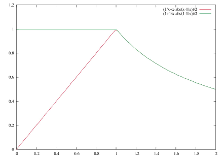
Figure 1: At the left we obtain the results for the SK model, at the right we have experimental data on metallic spin glasses [28]. The similarities among the two figures are striking.

3 Present theoretical understanding

3.1 General considerations

As we have already seen the actual solution of the SK model is a particular one, and in spite of its rather large complication, is the simplest one for a system with many equilibrium states. In principle one can consider more complex mean field solutions; sincerely I hope that these more complex solutions of the mean field equations are not necessary for spin glasses, but they could be useful in other contexts (e.g. in non equilibrium systems or in evolutionary systems with sexual reproduction [13]).

The basic principles, on which the theory is based, are the following:

• The function $P(q)$ is non-trivial and it changes from system to system.

• The system is stochastically stable, in presence of an infinitesimal magnetic field that breaks the spin reversal symmetry .

• Overlap equivalence states that all other possible definitions of overlaps are equivalent to the original one. i.e. in the infinite volume limit the new overlaps become given functions of the usual overlap $q$ [16].

• Ultrametricity, to be defined later.

This four principles are listed in order of relevance and generality. In principle it is possible that the last two could no be valid in sufficiently small dimensions and this would call for modifications of the field theory and (may be) for a more complex order parameter.

It is clear that at sufficiently low dimensions (e.g. for dimensions less that 2.5) the order parameter must be zero and mean field does not apply anymore, however some remnants of mean field theory may survive if the system is not too large or the observation time is not too long, as it happens for two dimensional superconductors where the Landau Ginsburg theory applies very well at low temperatures on human scales, in spite of the absence of an order parameter at equilibrium.

3.2 The probability distribution of the overlap

There are no doubts from simulations, also in three dimensions (at least at zero magnetic field) that the function $P_{j}(q)$ is non trivial and it fluctuates from system to system. In fig. (2) we show some data for two three-dimensional samples with side $L=16$. In fig. (3) we show the average function $P(q)$ in four dimensions.

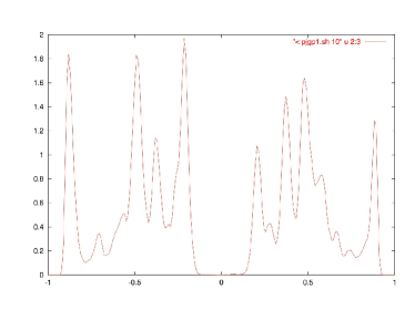
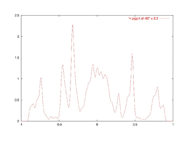
Figure 2: The function $P_{J}(q)$ for two samples samples (i.e a different choice of $J$) for $D=3,\ L=16$ ($16^{3}$ spins)[29].

This effect has been consistently seen in all the simulations for a quite large range of temperatures (practically up to $T=0$) and it persists also for larger lattices (the largest lattices where systematic investigations have been done have side $L=24$ in dimensions 3. There are very strong indications that this effect should persist in the infinite volume limit. Also the critics of the replica approach accept this point, which is not controversial anymore.

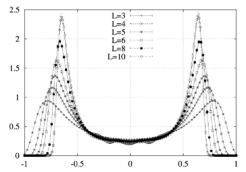
Figure 3: The function $P(q)=\overline{P_{J}(q)}$ for $D=4$ after average over many samples (L=3…10) [31].

3.3 Stochastic stability.

Stochastic stability is a very strong principle: it implies the existence of an infinite set of identities, maybe the most well known being:

$$P(q_{1,2},q_{3,4})\equiv\overline{P_{J}(q_{1,2})P_{J}(q_{3,4})}=\frac{2}{3}P(q_{1,2})P(q_{3,4})+\frac{1}{3}P(q_{1,2})\delta(q_{1,2}-q_{3,4})\ .$$ (5)

The function $P(q_{1,2},q_{3,4})$ can be measured in simulations in a rather simple way by considering 4 identic replicas (or clones) of the the same system (i.e. all with the same Hamiltonian). A direct test of this last relation is not simple, because delta function are rounded in finite volume system. Simpler relations are obtained by taking the moments. For example let us consider four replicas of the system. The previous equation implies that

$$\overline{\langle q_{1,2}^{2}q_{3,4}^{2}\rangle}=\frac{2}{3}\overline{\langle q_{1,2}^{2}\rangle}^{2}+\frac{1}{3}\overline{\langle q_{1,2}^{4})\rangle},$$ (6)

which is satisfied numerically with very high accuracy [32].

In some sense stochastic stability is not an assumption. If we consider the link overlap (to be defined later) at the place of the usual overlap, stochastic stability is a theorem in equilibrium system that has been recently proved [33]. Of course the theorem is valid in the infinite volume limit and finite volume corrections have not been evaluated, so that it is a welcome information to know that, at least as far the low moments are concerned as in equation eq. (6), the stochastic stabilities identities are satisfied with high precision also for not too large systems.

Stochastic stability is a very strong requirement, whose implication have not completely spelled out. We only notice here the very interesting fact that two non-interacting stochastically stable system do not form a single stochastically stable system, so that stochastically stability implies in some sense the existence of a certain degree of coherence of the system. Moreover let me mention (although this paper is devoted to statics) that stochastic stability gives the link to relate the equilibrium properties to the properties of systems that are slightly of equilibrium, recovering in this way the famous fluctuation dissipation relations [34, 35, 36, 37, 38]. More detailed consequences of stochastic stability are discussed in [39, 40].

3.4 Overlap equivalence

Of course there could be many definition of overlaps [13]. You may take any quantity $O(i)$ and define an $O$-dependent overlap as

$$q^{O}_{\alpha,\gamma}=N^{-1}\sum_{i}\langle O(i)\rangle_{\alpha}\langle O(i)\rangle_{\gamma}$$ (7)

A special case, that has been often investigated, is the link overlap, that on a $D$ dimensional lattice is defined as

$$q^{L}_{\alpha_{\gamma}}=1/(DN)\sum_{i,k}\langle\sigma(i)\sigma(k)\rangle_{\alpha}\langle\sigma(i)\sigma(k)\rangle_{\gamma}$$ (8)

where the sums goes on all the $DN$ links $i$ $k$ of the cubic lattice (i.e. all the pairs of nearest neighbour points).

Overlap equivalence state that in the infinite volume limit

$$q^{O}_{\alpha,\gamma}=f^{O}(q_{\alpha,\gamma})\ ,$$ (9)

where the function $f^{O}$ may depend on the temperature. In the case of the SK model we have the simple relation:

$$q^{L}_{\alpha_{\gamma}}=q_{\alpha,\gamma}^{2}\ .$$ (10)

This statement may be cast in a more explicit way if we consider the overlap correlation $G(x)$ defined in a system composed by two replicas of the same system (which for definiteness we call $\sigma$ and $\tau$):

$$G(x)=\langle\sigma(x)\tau(x)\sigma(0)\tau(0)\rangle\ .$$ (11)

We define also the constrained overlap correlation $G(x|q)$ where the previous average is done only on those pair of configurations that have overlap $q$. It can be shown that overlap equivalence is equivalent to the statement that the correlation functions are clustering in the this constrained ensemble [16] and therefore

$$\lim_{x\to\infty}G(x|q)=q^{2}\ .$$ (12)

It is interesting to note that the correlation at distance 1, $G(1|q)$, is also called the link overlap $Q_{L}(q)$. The previous relations implies that in the infinite volume limit

$$\langle q^{O}\rangle_{q}=f^{O}(q),\ \ \ \langle(q^{O})^{2}\rangle_{q}=\langle q^{O}\rangle_{q}^{2}\ .$$ (13)

In the same way in the ferromagnetic Ising model the violations of clustering and the presence of fluctuation in intensive quantities are eliminated by considering the constrained ensembles with positive (or negative) magnetization, therefore the sign of the magnetization is the order parameter. Here the situation is similar, but the constraint is the value overlap. In the ensemble of two replicas at fixed overlap intensive quantities do not fluctuate. This principle partially closes the Pandora box opened by the fact that in the usual unconstrained ensemble intensive quantities do fluctuate [1].

This picture implies that the probability distribution of the window overlaps, i.e. overlaps in a region of side $R$ when the side $L$ goes to infinity first, is similar to that a system with size $L$, a crucial prediction that has been directly checked [32, 41].

This scenario has been questioned and an alternative scenario, the TNT scenario, has been proposed [7]. According to this scenario the situation should be similar to the Ising ferromagnetic with antiperiodic boundary conditions: there are many states (the interface may be anywhere) and there is a non trivial $P(q)$. These states are locally identical (apart from a spin flip) with the exclusion of a region whose relative volume goes to zero as $L^{-a}$ with $a=1$. In the TNT scenario we would have that for $x<<L$, $G(x|q)$ does not depend on $q$ for not too large $q$, i.e. for $1<<x<<L$

$$G(x|q)=q_{ea}^{2}\ ,$$ (14)

while for $x$ of $O(L)$, $G(x|q)$ is a function of $x/L$.

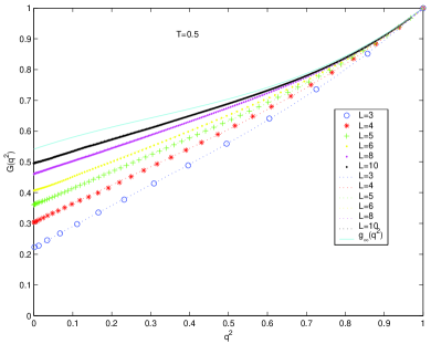
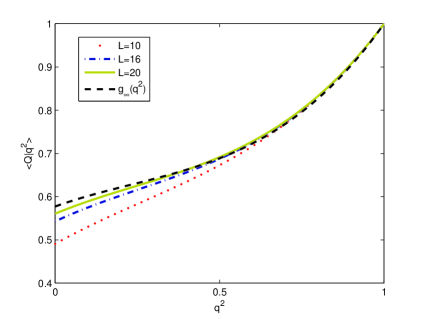
Figure 4: Plot of the curves $Q_{L}(q^{2})$ ( for $T=0.5$ Gaussian model): Left panel $L=3,10$ and infinite volume extrapolation) [44]. Right panel. Plot of the curves $Q_{L}(q^{2})$ ( for $T=0.5$ bimodal model): $L=10,20$ and infinite volume extrapolation) [45].

The TNT scenario, in spite of the difficulties to put it in a stochastically stable form, had some popularity a few years ago, when it was proposed for the first time. It would predict a delta function probability distribution for the link overlap. However this conclusions were based on not too large lattices. A more complete analysis already showed that the arguments for the TNT scenario were related to transient finite volume effects [42]. Indeed it now very clear, both from data for small lattices but at low temperature [43] and from data on quite larger lattices (i.e. up to $L=20$) [44, 45] that the TNT scenario is no correct and that for $q$ not very near to $q_{EA}$ we have

$$\langle Q^{L}(q)\rangle=A+B\,q^{2}\ ,$$ (15)

where $B$ has a definite limit when $L$ goes to infinity (see fig. (4)). Moreover the fluctuations of $Q^{L}(q)$, i. e. its variance, go to zero quite fast with the side (something like $L^{-1.4}$, see fig. (5)).

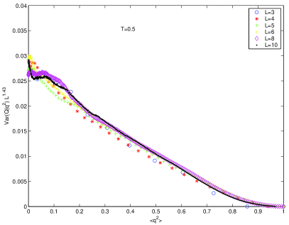
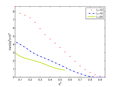
Figure 5: Variance of $Q_{L}(q^{2})$ (left panel divided by $L^{1.43}$ for the temperature $T=0.5$ [44], right panel not divided by $L^{1.43}$ for the temperature $T=0.7$ [45]), as a function of $q^{2}$, for different sizes $L$.

3.5 Dynamic correlations

A particular interesting case are the correlations at at $q=0$. According to the clustering properties they should go to zero at infinity, as a power with an exponent that can be estimated analytically:

$$G(x|0)\propto x^{-\alpha}\ .$$ (16)

The interest on these correlations is that they can be computed in the dynamics [46]: indeed if one consider a pairs of two large large systems, if $q=0$ at time zero, $q$ remains zero at all times. Therefore one can wait for a long time and compute the equal time correlation function. Obviously they will remain nearly equal to zero at distances larger that the dynamically growing correlation length $\xi(t)$. By definition in the limit $t\to\infty$ and fixed $x$ we obtain equilibrium correlations in some equilibrium state.

In the TNT scenario the correlation functions are the same in all equilibrium states in the infinite volume limit and for not to small $x$ they are given by $G(x)=q_{EA}^{2}$; therefore we must have

$$G(x,t)=q_{EA}^{2}f(x/\xi(t))\ .$$ (17)

On the contrary if overlap equivalence holds we should have

$$G(x,t)={x^{-\alpha}}f(x/\xi(t))\ .$$ (18)

There is in the literature no indications whatsoever that eq. (17) holds for the correlations; all numerical simulations (which have done in quite diverse situations) consistently support eq. (18).

However someone may object that in most cases the correlations functions are measured not at too large distances, so that a fit may be ambiguous. A very interesting test of the theoretical predictions can be done in one dimensional models with long range interactions. If we use the diluted version [48] of Young long range model [47], one can easily measure the correlations functions at distances $10^{5}$ (linear lattices with $N=10^{6}$ sites can be simulated). The model is such that

$$\overline{J(i,)^{2}}\propto|i-k|^{-\rho}\ .$$ (19)

More precisely in the diluted version $J_{i,k}=\pm 1$ with probability $|i-k|^{-\rho}$, otherwise it is zero [48].

This model is a proxy of the $D$ dimensional short range model model, with the relation $\rho=1+2/D$, in the sense that the two models have the same upper critical dimension, although they may have a different lower critical dimension.

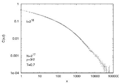
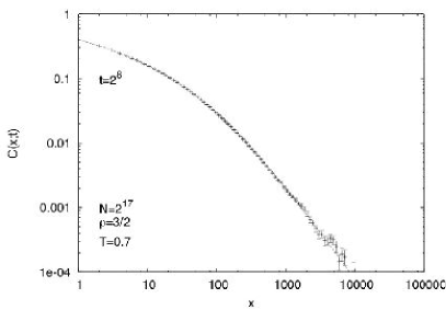
Figure 6: The correlation functions on a one dimensional lattices with $N=2^{17}$ and $\rho=1.5$ in the low temperature phase ($T\approx.4T_{c}$) at time $t=2^{18}$, left panel, and at time $t=2^{8}$, right panel, as function of the distance, fitted with formula eq. (20).

The data may be very well fitted for 4 decades in $x$ by

$$G(x,t)=ax^{-\alpha}\left(1+(x/\xi(t))^{\delta(\rho-\alpha)}\right)^{-1/\delta}\ ,$$ (20)

where we have imposed at very large distances $G(x,t)\propto x^{-\rho}$ (see for example fig. (6)). It turns out that $\alpha$ is roughly temperature independent below and not near to $T_{c}$. The correlation function (at least at some temperatures) seems to increase as stretched power. i.e as $\xi(t)\propto B\exp(A\log(t)^{1/2})$.

The conclusion is quite clear: the dynamic correlation function behaviour in a way that is quite different from that of the droplet model and of TNT scenario and they are perfectly consistent with the clustering properties of the replica approach. Two different copies evolve locally toward two different incongruent ground states.

4 Ultrametricity

Ultrametricity states a very striking property for a physical system: essentially it says that the equilibrium configurations of a large system can be classified in a taxonomic (hierarchical) way (as animals in different taxa): configurations are grouped in states, states are grouped in families, families are grouped in superfamilies.

Ultrametricity implies that sampling three configurations with respect to their common Boltzmann-Gibbs probability, the distribution of the distances among them is supported, in the limit of very large systems, only on equilateral and isosceles triangles with no scalene triangles contribution.

We define the three replicas overlap distribution ${\cal P}_{3}$.

$${\cal P}_{3}(q_{1,2},q_{2,3},q_{3,1})=\langle\delta(q_{1,2}-q(\sigma,\tau))\delta(q_{2,3}-q(\tau,\gamma))\delta(q_{3,1}-q(\gamma,\sigma))\rangle\;,$$ (21)

where $\sigma,\tau,\gamma$ denote three different equilibrium configurations.

Ultrametricity implies that ${\cal P}_{3}$ is zero when the following inequality is violated

$$q_{1,3}\geq\max(q_{1,2},q_{2,3})$$ (22)

Stochastic stability implies [49] an exact formula for $\overline{{\cal P}_{3}}$:

$$\overline{{\cal P}_{3}}(q_{1,2},q_{2,3},q_{3,1})=\frac{X(q_{1,2}}{2}P(q_{12})X(q_{1,2})\delta(q_{1,2}-q_{2,3})\delta(q_{2,3}-q_{3,1})+$$

$$\frac{1}{2}P(q_{1,2})P(q_{2,3})\theta(q_{1,2}-q_{2,3})\delta(q_{2,3}-q_{3,1})$$

$$\frac{1}{2}P(q_{2,3})P(q_{3,1})\theta(q_{2,3}-q_{3,1})\delta(q_{3,1}-q_{1,2})$$ (23)

$$+\frac{1}{2}P(q_{3,1})P(q_{1,2})\theta(q_{3,1}-q_{1,2})\delta(q_{1,2}-q_{2,3}),$$

where $X(q)=\int_{0}^{q}P(q)dq^{\prime}$.

There are some indications that suggest that, for a stochastically stable system overlaps equivalence should imply ultrametricity [50], however no mathematical theorem exists.

There were in the literature some direct test of ultrametricity in dimensions $4$ [51] and some indications (coming from the dynamics [52]) of the validity of ultrametricity in D=3. It is therefore interesting to test directly if ultrametricity present in D=3.

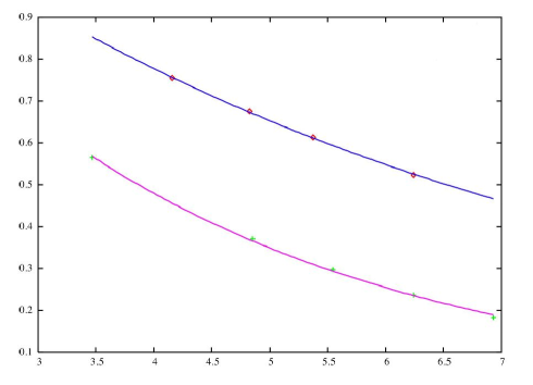
Figure 7: Data extracted from [51]: the average value of $K$ (including the point $K=1$, as function of the volume in the SK model (lower curve) and in the $3d$ EA model (upper curve). The curves are power fits to the data.

There have been some simulations in which the ultrametricity property was investigated [53] by trying to identify the states and to define an ultrametricity index $K$ that takes values in the interval $[0-1]$ such that the $K=0$ correspond to ultrametricity. The simulations were done at low temperature in small lattices.

The expectation values of $K$ as function of the size of the system are shown in fig (7) both for the SK model and for the 3 dimensional Ising model. Both data are well fitted by a power of the volume

$$\langle K\rangle\propto N^{-\lambda}$$ (24)

with $\lambda=.31$ in the SK model and $\lambda=.17$ in $d=3$ (in other words $K\propto L^{-.5}$). The data suggest that $\langle K\rangle$ goes to zero in the infinite volume limit also in $D=3$ although for $L=8$, the maximum lattice explored the value of $K$ is not small. The reader should notice that these are not the conclusions of the authors of the paper [51]: they concentrated their attention on the expectation of value of $K$ restricted to those configurations which have $K<1$ and with this restriction the behaviour is not so simple. Although the difference between the two quantities does not matters in the limit where $K$ goes to zero, the restriction of considering only the data with $K<1$ introduce a finite volume distortion and it may hide a simple power behavior.

As far as the extrapolation a $K=0$ starting from large values of $K$ could be dangerous, it is interesting to study directly the ultrametricity on a larger lattice, using also a less sophisticated analysis that has a simple direct interpretation.

This was done in [45]. We considered three independent configurations 1, 2, 3 such that

$$|q_{1,2}|<|q_{1,3}|<|q_{2,3}|\ ,$$ (25)

If we flip the configurations in such a way that $0<q_{1,3}<q_{2,3}$, it turns out that below the critical temperature $q_{1,2}$ is positive, or, if negative, very near to zero. As far ultrametricity implies that $q_{1,2}=q_{1,3}$ a natural ultrametricity index is given by

$$U=\frac{\langle(q_{1,2}-q_{1,3})^{2}}{\langle q^{2}\rangle}\ .$$ (26)

We have measured $U$ for lattices going from $L=4$ to $L=20$ for temperatures up to $.6T_{c}$, see fig. (8).

At $T_{C}$ the probability distribution is not ultrametric but it nearly ultrametric: the value of $U$ is at the fixed point is much smaller that the value at the high temperature Gaussian fixed point (i.e. around .8) Ultrametricity seems to be present below $T_{c}$, but it sets in slowly like $L^{-.3}$ . In may be possible that the small power of $L$ is an artifact of being too near to the critical temperature and that the exponent of the power may be slightly high at smaller temperatures, showing a more fast approach to ultrametricity.

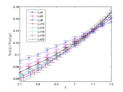
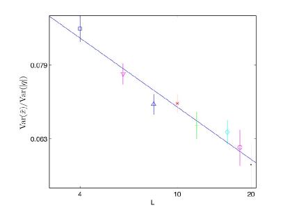
Figure 8: The ultrametricity index $U$ as function of the temperature and of the volume (left panel); the curves crosses at the the critical point. The ultrametricity index $U$ as function of the size of the lattice at $T=.7$ (right panel), where the line is a fit proportional to $L^{-.3}$.

5 Conclusions and questions to be answered

Replica symmetry breaking picture is confirmed. Good evidence if found for overlap equivalence and alternative interpretative scheme like the droplet model or the $TNT$ scenario are no more viable.

Ultrametricity seems to present in the statics. However the measurements are difficult, there are strong finite volume corrections). In the future, we must recheck the $D=4$ short range model and study the long range 1D model for different values of $\rho$. Given the slow approach to ultrametricity in the static one may wonder what happens in the dynamics. Can one use the measured violation of ultrametricity at finite volume in the statics to compute the violations of dynamical ultrametricity in the dynamics?

A very important issue is the behaviour of spin glass in magnetic field. It is possible that in the same way that a random magnetic field destroys the ferromagnetic order in D=2, a random (or constant) magnetic field may destroy spin glass order $D=3$.

In the last year some simulations papers appeared claiming that the de Almeida line, that should separate the replica exact from the replica broken regions is not present in D=3 [47, 54]. I would be more prudent to reach these conclusions:

• For finite volume there is a cross-over region where configurations with negative magnetization have an important role also in presence of a small non zero magnetic field. Any analysis done inside this region may be quite dangerous.

• There are analysis done on very large lattice with a different methodology that indicate that a transition is present in magnetic field and these analysis cannot be easily dismissed [55].

• The previous analysis [55] showed that in presence of a magnetic field the effects of replica symmetry breaking are strongly decreasing with decreasing the dimension, so is not clear if the analysis that miss the $dAT$ transition have enough sensitivity to detect it.

This problem should be carefully investigated and now we have all the tools to investigate the problem more deeply. It remains however a problem quite difficult to be studied, the window of magnetic fields (not too small, not to big) for which sensible results may be obtained may be small in simulations.

Generally speaking analytic progresses are also deeply needed: the development of a non-linear sigma model at low temperature and of a real space renormalization group results are are very important steps that should be achieved.

We should be grateful to David for having given to us something interesting to work on not only in the last 30 year, but also for the next 30 years.

References

- [1] Mézard, M., Parisi, G. and Virasoro, M.A. (1987) Spin Glass Theory and Beyond, (World Scientific, Singapore).
- [2] Parisi G. (1992) Field Theory, Disorder and Simulations, (World Scientific, Singapore).
- [3] G. Parisi in Les Houches Summer School - Session LXXVII: Slow relaxation and non equilibrium dynamics in condensed matter, ed. by J.-L. Barrat, M.V. Feigelman, J. Kurchan, and J. Dalibard, Elsevier 2003.
- [4] G.Parisi PNAS 103 7948 (2006).
- [5] G. Parisi in Les Houches Summer School - Session LXXVII: Slow relaxation and non equilibrium dynamics in condensed matter, ed. by J.-L. Barrat, M.V. Feigelman, J. Kurchan, and J. Dalibard, Elsevier 2007.
- [6] D.S. Fisher, D.A. Huse, Phys. Rev. Lett 56, 1601 (1986); Phys. Rev. B 38, 373 (1988).
- [7] F. Krzakala and O. C. Martin, Phys. Rev. Lett. 85, 3013 (2000). M. Palassini and A. P. Young, Phys. Rev. Lett. 85, 3017 (2000).
- [8] S. F. Edwards and P. W. Anderson, J. Phys. F 5, 965 (1975).
- [9] Sherrington D. and Kirkpatrick S. (1975) Phys. Rev. Lett., 35, 1792; Kirkpatrick S. and Sherrington D. Phys. Rev. B 17, (1978)
- [10] R.L. de Almeida, D.J. Thouless, J. Phys. A 11 (1978) 983.
- [11] Thouless D.J.,Anderson P. A. and Palmer R. G. (1977) Phil. Mag. 35, 593.
- [12] Anderson P.W. (1979), in Ill condensed matter, eds Balian R., Maynard R and Toulouse G., (North-Holland, Berlin) pp. 159-259.
- [13] G. Parisi, Physica Scripta 35, 123 (1987).
- [14] F. Guerra, Int. J. Mod. Phys. B 10, 1675 (1997).
- [15] Aizenman M. and Contucci P. (1998) J. Stat. Phys, 92, 765.
- [16] Parisi G. Int. Jou. Mod. Phys. B, 18, 733-744, (2004).
- [17] Guerra F. (2002) Comm. Math. Phys. 233 1.
- [18] Talagrand M. (2006), Ann. of Math., 163 221.
- [19] C. De Dominicis, I. Kondor, and T. Temesv ari, Beyond the Sherrington-Kirkpatrick Model (World Scientific, 1998), vol. 12 of Series on Directions in Condensed Matter Physics, p. 119, cond-mat/9705215; Eur. Phys. J. B 11, 629 (1999).
- [20] T. Temesv ari and C. De Dominicis, Phys. Rev. Lett. 89, 097204 (2002).
- [21] S. Franz, G Parisi, M.A. Virasoro, .J. Phys. France 4, 1657 (1994).
- [22] S. Boettcher Stiffness of the Edwards-Anderson Model in all Dimensions cond/mat 0508061.
- [23] Aizenman M. , Sims R. , Starr S. L.(2003) Phys. Rev. B 68, 214403.
- [24] D. Sherrington: Magnets, microchips, memories and markets: statistical physics of complex systems, Bakerian lecture (2001)
- [25] C. De Dominicis and I. Kondor, Phys. Rev. B 27, 606 (1983).
- [26] C. De Dominicis, I. Giardina, E. Marinari, O. C. Martin, F. Zuliani Phys. Rev B 72, 014443 (2005).
- [27] D. Ruelle, Comm. in Math. Phys., 5, 324 (1967).
- [28] C. Djurberg, K. Jonason and Nordblad P. (1998) Eur. Phys. J. B 10, 15.
- [29] Marinari E., Parisi G. and Ruiz-Lorenzo J.J. (1998) in Spin Glasses and Random Fields, ed. P. Young (World Scientific, Singapore ) pp. 58.
- [30] L. Gnesi, R. Petronzio and F. Rosati Evidence for Frustration Universality Classes in 3D Spin Glass Models cond-mat/0208015.
- [31] Marinari E., Zuliani F. (1999) J. Phys. A 32, 7447-7461.
- [32] Marinari E., Parisi G., Ricci-Tersenghi F., Ruiz-Lorenzo J. and Zuliani F. (2000) J.Stat. Phys 98, 973.
- [33] P. Contucci, J. Phys. A: Math. Gen. 36, 10961, (2003); P. Contucci, C. Giardinà, Jour. Stat. Phys. to appear math-ph/05050 (2005).
- [34] Cugliandolo L.F. and Kurchan J.(1993) Phys. Rev. Lett. 71, 173.
- [35] Cugliandolo L.F. and Kurchan J.(1994) J. Phys. A: Math. 27, 5749.
- [36] Franz S. and Mézard M. (1994) Europhys. Lett. 26, 209.
- [37] Franz S., Mézard M., Parisi G., Peliti L. (1999), J. Stat. Phys. 97 459.
- [38] D. Hérisson and M. Ocio, Phys. Rev. Lett. 88, 257202 (2002).
- [39] Parisi G. (2003) J. Phys. A 36 10773.
- [40] G.Parisi (2004) Europhys. Lett. 65, 103.
- [41] E. Marinari, G. Parisi, F. Ricci-Tersenghi, J. J. Ruiz-Lorenzo, J. Phys. A: Math. and Gen. 31 (1998) L481.
- [42] Marinari E., Parisi G., Phys. Rev. B 62, 11677 (2000), Phys. Rev. Lett. 86 (2001) 3887.
- [43] G.Hed and E-Domany ”Both site and link overlap distributions are non trivial in 3-dimensional Ising spin glasses” cond-mat/0608535v4 (2007)
- [44] P. Contucci, C. Giardinà, C. Giberti, C. Vernia Phys. Rev. Lett. 96, 217204 (2006).
- [45] P. Contucci, C. Giardinà, C. Giberti, G. Parisi, C. Vernia Ultrametricity in the Edwards-Anderson Model, cond-mat/0607376, Phys. Rev. Lett. (in press).
- [46] E. Marinari, G. Parisi, F. Ritort, J. Ruiz-Lorenzo Phys. Rev. Lett. 76 (1996) 843; E. Marinari, G. Parisi, F. Ricci-Tersenghi, J. J. Ruiz-Lorenzo, J. Phys. A. 33, 2373 (2000); E. Marinari, G. Parisi, J. J. Ruiz-Lorenzo Journal of Physics A 35, 6805-6814 (2002)
- [47] Helmut G. Katzgraber, A. P. Young Phys. Rev. B 72, 184416 (2005).
- [48] L. Leuzzi, G. Parisi, F. Ricci Terzenghi J. J. Ruiz-Lorenzo, in progress.
- [49] Iniguez D., Parisi G. and Ruiz-Lorenzo J.J.(1996) J.Phys. A29 4337.
- [50] G. Parisi and F. Ricci-Tersenghi J. Phys. A 33 113 (2000).
- [51] A. Cacciuto, E. Marinari, G. Parisi J. Phys. A: Math. Gen 30 L263-L269 (1997).
- [52] S. Franz, F. Ricci-Tersenghi, Phys. Rev. E 61, 1121 (2000).
- [53] G. Hed, A. P. Young, E. Domany Phys. Rev. Lett. 92, 157201 (2004).
- [54] A. P. Young, Helmut G. Katzgraber, Phys. Rev. Lett. 93, 207203 (2004).
- [55] E. Marinari G. Parisi , F. Zuliani J. Phys. A:31 (1998) 1181; E. Marinari, G. Parisi, F. Zuliani Phys. Rev. Lett. 84 (2000) 1056; G. Parisi, F, Ricci-Tersenghi, J. J. Ruiz-Lorenzo Phys. Rev. B 57, 13617 (1998); E. Marinari, C. Naitza, F. Zuliani J. Phys. A: Math. Gen. 31 (1998) 6355; F. Krzakala, J. Houdayer, E. Marinari, O.C. Martin, G. Parisi Phys. Rev. Lett. 87, 197204 (2001)