Magnetic resonance as an orbital state probe

Abstract

Magnetic resonance in ordered state is shown to be the direct method for distinguishing the orbital ground state. The example of perovskite titanates, particularly, LaTiO₃ and YTiO₃, is considered. External magnetic field resonance spectra of these crystals reveal glaring qualitative dependence on assumed orbital state of the compounds: orbital liquid or static orbital structure. Theoretical basis for using the method as an orbital state probe is grounded.

Recently, a lot of spin and orbital phases and their phase transitions attract intent investigation due to interplay of these degrees of freedom, particularly in transition-metal (TM) oxides. Imada et al. (1998) Fundamental physical properties revealed in such systems are still a subject for a discussion. Among the phenomena which attract the most attention there is a superexchange interactions driven rich spin-orbital quantum phase diagram proposed to exist in perovskite titanates and vanadates. Khaliullin and Maekawa (2000); Khaliullin and Okamoto (2003); Oleś et al. (2005)

Whether orbital liquid state present in real compound or not — is the question which have given rise to hot debates especially concerning the simpler system — $R\text{TiO}_{3}$, $R$ is rare-earth element or Y.

In wide temperature range for different $R$, titanates are known to possess orthorhombic crystal structure  Komarek et al. (2007); Cwik et al. (2003) (which is often called ”quasi-cubic”) with Pnma space group (see Fig. 1). GdFeO₃-type distortions ($T_{1g}$-distortions), which are present in these crystals, are believed to control magnetic structure and properties of the compounds through the influence on their orbital ground state. Imada et al. (1998); Mochizuki and M.Imada (2003, 2004)

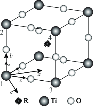
Figure 1: $R$TiO₃ crystal structure. Pnma (a, b, c) and pseudocubic (x, y, z) axes are shown. Numbers denote Ti sublattices.

The discussion of titanates orbital ground state was started by Khaliullin and Maekawa Khaliullin and Maekawa (2000) who proposed the superexchange model with dynamical quenching of local orbital moments in a simple cubic lattice of Ti³⁺ ions with no static orbital order but with fixed magnetic arrangement — in contrast to usual Goodenough-Kanamori picture. This approach based on the Kugel-Khomskii model Kugel and Khomskii (1982) perfectly explains the unusual reduction of Ti³⁺ spin Meijer et al. (1999); Ulrich et al. (2002) and anomalous isotropic spin-wave spectrum Keimer et al. (2000) found experimentally, but contradicts to NMR Kiyama and Itoh (2003) and XAS Haverkort et al. (2005) experiments as well as some crystal-field Mochizuki and M.Imada (2003, 2004); Schmitz et al. (2005, ) and density-functional Solovyev (2006); Streltsov et al. (2005) calculations. However, it is supported by recent Raman scattering experiments Ulrich et al. (2006) revealing orbital excitations and thus making some orbital fluctuations possible.

In this context La and Y titanates are believed to be of special interest for investigators as these two ions stand at the opposite ends of rare-earths and Y series with different ionic radii. $T_{1g}$-distortions in YTiO₃ with ”smaller” Y are much greater of these in LaTiO₃, which has the biggest radius of $R$-ion in the whole series. One more feature which makes these two crystals more interesting is their magnetic ground states: lanthanum titanate is antiferromagnetic Cwik et al. (2003) with strong isotropic superexchange J of about $15.5$ meV, Keimer et al. (2000) whereas yttrium titanate is ferromagnetic with $J\approx-2.75$ meV. Ulrich et al. (2002) Moreover, almost isotropic superexchange couplings both in LaTiO₃ and its sister compound are in contrast with the situation in manganites and cuprates which have pronounced superexchange anisotropy.

Keeping in mind a huge collection of all above mentioned facts, one still can not find a compromise between them and can not answer what ground state is actually realized in titanates. That indicates a puzzling situation: on the one hand the system is already studied in many aspects, on the other hand some of its properties are not clear yet. To meet this challenge, the definite model of a titan perovskite oxide is developed in the current paper on the particular example of Y and La compounds

We start from the crystal-field Hamiltonian with explicit electron-lattice interaction, that is vibronic Hamiltonian (VH):

$$H_{vib} = H_{lin}+H_{QQ}+H_{R}=$$ (3)

$$= \left[V_{e}\left(Q_{\theta}X_{\theta}+Q_{\epsilon}X_{\epsilon}\right)+V_{t}\left(Q_{\xi}X_{\xi}+Q_{\eta}X_{\eta}+Q_{\zeta}X_{\zeta}\right)\right]+$$

$$+ \left[\begin{array}[]{l}V_{a}\left(Q^{2}_{x}+Q^{2}_{y}+Q^{2}_{z}\right)X_{A1}+V_{b}\left\{\left(2Q^{2}_{z}-Q^{2}_{x}-Q^{2}_{y}\right)X_{\theta}+\sqrt{3}\left(Q^{2}_{x}-Q^{2}_{y}\right)X_{\epsilon}\right\}+\\ V_{c}\left(Q_{y}Q_{z}X_{\xi}+Q_{x}Q_{z}X_{\eta}+Q_{x}Q_{y}X_{\zeta}\right)]\end{array}\right]+$$

$$+ \left[\begin{array}[]{l}{V_{e}}^{R}\left(Q^{R}_{\theta}X_{\theta}+Q^{R}_{\epsilon}X_{\epsilon}\right)+\\ {V_{t}}^{R}\left\{\left(Q^{R}_{\xi,1}+Q^{R}_{\xi,2}\right)X_{\xi}+\left(Q^{R}_{\eta,1}+Q^{R}_{\eta,2}\right)X_{\eta}+\left(Q^{R}_{\zeta,1}+Q^{R}_{\zeta,2}\right)X_{\zeta}\right\}\end{array}\right]~{}.$$ (6)

Here $Q_{\Gamma}$ and $Q^{R}_{\Gamma}$ ($\Gamma=\theta,\epsilon,\xi,\eta,\zeta,x,y,z$) are symmetrized shifts of oxygen and $R$-ions which are nearest and next-nearest Ti³⁺ neighbours correspondingly. These shifts are obtained from accurate crystal structure data for LaTiO₃ Cwik et al. (2003) and YTiO₃. Komarek et al. (2007) $X_{\Gamma}$ are symmetric orbital operators, acting on the 3d-$t_{2g}$ triplet, and $V_{\alpha}$ ($\alpha=e,t,a,b,c$) and $V^{R}_{\alpha}$ ($\alpha=e,t$) are electron-lattice coupling constants. Nikiforov et al. (1980) The first two square brackets, which are $H_{lin}$ and $H_{QQ}$, represent Ti³⁺ 3d-$t_{2g}$ electron interactions with nearest oxygen linear and quadratic symmetric shifts correspondingly, whereas $H_{R}$ is responsible for this electron and $R$-ions shifts coupling.

This Hamiltonian with ab initio $V_{\alpha}$ (calculated with GAMESS package Schmidt et al. (1993); Schmidt and Gordon (1998)) gives ground state with static orbital structure of the form predicted by Mochizuki and Imada, Mochizuki and M.Imada (2003, 2004) that is the following orbital functions (3d-$t_{2g}$ cubic basis set): $\psi_{1,2}(\text{La})=\psi_{3,4}(\text{La})\approx 1/\sqrt{3}\left(-\xi-\eta\pm\zeta\right)$, which is almost trigonal, in LaTiO₃ and $\psi_{1,2}(\text{Y})\approx 1/\sqrt{2}\left(\mp\xi+\zeta\right)$, $\psi_{3,4}(\text{Y})\approx 1/\sqrt{2}\left(\mp\eta+\zeta\right)$ — in YTiO₃. Here sign alternation reads sites 1(2) – the upper sign, and 3(4) – the lower one.

We have irrefutable argument for reproducing results of previous LDA-based  Haverkort et al. (2005); Solovyev (2006); Streltsov et al. (2005) or point-charges  Mochizuki and M.Imada (2003, 2004); Schmitz et al. (2005, ) investigations by using (6). All these studies either were based on oversimplified model Mochizuki and M.Imada (2003, 2004) (giving unlikely structure parameters) or did not reveal the mechanisms of the ground state formation. Haverkort et al. (2005); Schmitz et al. (2005, ); Solovyev (2006); Streltsov et al. (2005) The present calculation based on (6) showed that $H_{R}$ plays crucial role in the formation of solitary orbital singlet with its segregation at $\approx 0.20$ eV in LaTiO₃ and $\approx 0.15$ eV in YTiO₃. A half of these gaps is produced by the $R$-ion crystal field. The influence of the remainder of the crystal on Ti³⁺ orbital state is negligible.

Using the low-energy spectrum obtained from (6) we then exploit common Kugel-Khomskii (KK) method within the Hubbard model. Kugel and Khomskii (1982) Thus, arriving to isotropic superexchange, one then can perform Moriya’s approach Moriya (1960) for treating antisymmetric terms Nikiforov et al. (1971) of the effective $S\text{-}\frac{1}{2}$ spin-Hamiltonian (ESH) introduced below:

$$H_{ef\!f}=J_{ij}\left({\bf S}_{i}\cdot{\bf S}_{j}\right)+{\bf D}_{ij}\left({\bf S}_{i}\times{\bf S}_{i}\right)+S^{\alpha}_{i}A^{\alpha\beta}_{ij}S^{\beta}_{j}+H^{\alpha}_{i}g^{\alpha\beta}_{i}S^{\beta}_{i},$$ (7)

where $J_{ij}$ stands for isotropic superexchange between $i$-th and $j$-th magnetic ions, ${\bf D}_{ij}$ is Dzyaloshinskiy-Moriya vector, ${\textsf{A}}_{ij}$ is symmetric anisotropy tensors, ${\textsf{g}}_{i}$ is g-factor and $\bf H$ represents external magnetic field.

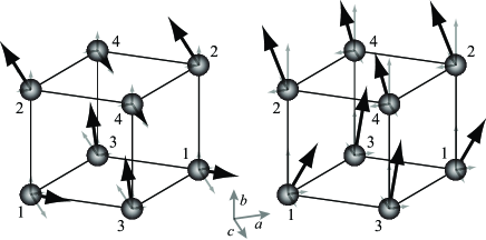
Figure 2: Schematic magnetic structures of LaTiO₃ (up) and YTiO₃ (bottom). Gray arrows denote magnetization projections (Pnma).

The Hubbard model parameters: energy of electron hopping from the $m$-th orbital on one site to the $n$-th on the neighboring one in strictly cubic system $t_{mn}$, on-site Coulumb repulsion of a pair of electrons U and intra-atomic electronic exchange interaction ${\text{J}}_{\text{H}}$ — are taken from LDA-based calculation. Solovyev (2006) For LaTiO₃ $t_{mm}\approx 0.25$ eV, $t_{m\neq n}\approx 0.12$ eV, ${\text{U}}\approx 3.20$ eV, ${\text{J}}_{\text{H}}\approx 0.61$ eV. For YTiO₃ $t_{mm}\approx 0.27$ eV, $t_{m\neq n}\approx 0.08$ eV, ${\text{U}}\approx 3.45$ eV, ${\text{J}}_{\text{H}}\approx 0.62$ eV. Indexes in $t_{mn}$ denote 3d-$t_{2g}$ orbitals, namely $\xi$, $\eta$, $\zeta$. All interactions in ESH, which follow from these parameters, are listed in Tables 1, 2.

Table 1: Single crystal g-factors of LaTiO₃ and YTiO₃. The Pnma coordinate system is used.

$R$	La	Y
${\textsf{g}}_{i}$	$\left(\begin{array}[]{ccc}1.93&0.03&-0.05\\ 0.03&1.89&-0.04\\ -0.05&-0.04&1.93\end{array}\right)$	$\left(\begin{array}[]{ccc}1.93&-0.04&-0.04\\ -0.04&1.87&0.02\\ -0.04&0.02&1.96\end{array}\right)$

This calculation of superexchange couplings, although it is not something new, is to be reproduced because of extreme sensitivity of these parameters to the orbital state. This well-known feature of the KK treatment should be considered as (in comparison with previous studies  Mochizuki and M.Imada (2003, 2004); Haverkort et al. (2005); Schmitz et al. (2005, ); Solovyev (2006); Streltsov et al. (2005); Eremina et al. (2004)) we have obtained new $\psi_{i}(\text{La})$ and $\psi_{i}(\text{Y})$ , $i=1\ldots 4$.

Table 2: Magnetic interactions (meV) in LaTiO₃ and YTiO₃. The Pnma notations are used.

$R$	$J_{12}$	$J_{12}$	${\bf D}_{12}$	${\bf D}_{13}$	${\textsf{A}}_{12}$	${\textsf{A}}_{13}$
La	13.21	16.12	$\left(\begin{array}[]{c}0.58\\ 0\\ -2.80\end{array}\right)$	$\left(\begin{array}[]{c}0\\ -0.36\\ -0.17\end{array}\right)$	$\left(\begin{array}[]{ccc}-0.07&0&0.06\\ 0&-0.08&0\\ 0.06&0&-0.34\end{array}\right)$	$\left(\begin{array}[]{ccc}-0.02&0&0\\ 0&-0.03&-0.02\\ 0&-0.02&-0.01\end{array}\right)$
Y	-2.77	-2.72	$\left(\begin{array}[]{c}0.60\\ 0\\ -0.21\end{array}\right)$	$\left(\begin{array}[]{c}0\\ -0.38\\ -0.11\end{array}\right)$	$\left(\begin{array}[]{ccc}-0.21&0&0.06\\ 0&-0.03&0\\ 0.06&0&-0.06\end{array}\right)$	$\left(\begin{array}[]{ccc}-0.69&0&0\\ 0&-0.10&-0.09\\ 0&-0.09&-0.16\end{array}\right)$

By using the Hamiltonian (7) one can obtain magnetic ground state as well as magnetic excitations in both compounds. The magnetic structure type for both crystals is $(A_{x},F_{y},G_{z})$ with major $G$-component in LaTiO₃ and $F$ — in YTiO₃ (see Fig. 2) — in excellent agreement with neutron scattering experiments. Meijer et al. (1999); Ulrich et al. (2002) Here we should emphasize two special features in $J_{ij}$ which are crucial for obtaining correct magnetic structure. First is considering Hund’s coupling, which is ${\text{J}}_{\text{H}}/{\text{U}}$ smaller then ”common” superexchange, Anderson (1959) proportional to $t^{2}_{mn}/{\text{U}}$ for titanates. The second is explicit introduction of the Ti–O–Ti bond angle ($\varphi$) –dependence of $t_{mn}$. Moskvin and Bostrem (1977) These two give for a pair of Ti³⁺ ions along the b axis (Pnma):

$$J_{12}=a\left(b-\frac{{\text{J}}_{\text{H}}}{\text{U}}\right)-c\left(d+\frac{{\text{J}}_{\text{H}}}{\text{U}}\right){\sin}^{2}\varphi,$$ (8)

where $a=3.54(2.61)$, $b=6.37(1.66)$, $c=43.30(14.70)$ and $d=0.84(0.92)$ are numeric coefficients for La(Y) compound. These coefficients depend on the particular Ti³⁺ orbital state, on $t_{mn}$ and U. Ti–O–Ti bond angle $\varphi$ for lanthanum titanate is about $153^{\circ}$ and $142^{\circ}$ for YTiO₃. Without ${\text{J}}_{\text{H}}$ one can not obtain experimentally observed magnetic structure in both compounds simultaneously as Schmitz et al. Schmitz et al. (2005, ) couldn’t. And in strictly cubic system (without ${\sin}^{2}\varphi$–dependence of $J_{ij}$) one is not able to obtain the correct orbital structure as Khaliullin and Maekawa couldn’t Khaliullin and Maekawa (2000) for LaTiO₃.

It is important to mention that both anisotropic terms of the ESH, namely Dzyaloshinskiy-Moriya interaction and symmetric anisotropy, should be considered, otherwise the static magnetic order couldn’t exist. Shekhtman et al. (1992) This is not always kept by investigators. Ulrich et al. (2002); Keimer et al. (2000)

Actually, the above result is not unique as its different parts were obtained by several authors.  Mochizuki and M.Imada (2003, 2004); Schmitz et al. (2005, ); Solovyev (2006); Streltsov et al. (2005); Eremina et al. (2004) It is reproduced to illustrate the realistic model with reasonable parameters. But this model reveals particular mechanisms of titanates orbital and magnetic ground state formation that was not performed before.

Now we turn to the core idea of the paper. That is drastic dependence of the particular kind of magnetic excitations on orbital ground state.

We consider magnetic excitations, namely spin waves (SW) and antiferromagnetic/ferromagnetic resonance (AFMR/FMR) spectra, in LaTiO₃ and YTiO₃ exploiting linear approximation. Simulations (see Figs. 3, 4) turned out to be surprising when comparing the real static orbital structure with hypothetic orbital liquid state. The latter was simulated by averaging the superexchange parameters through low-energy part of the spectrum (6).

Figure 3: (Color online) Spin wave dispersions for LaTiO₃ (up) and YTiO₃ (bottom). Circles denote experimental data, taken from Ref. Keimer et al., 2000 for LaTiO₃ and from Ref. Ulrich et al., 2002 for YTiO₃. Simulated curves are black for static orbital order and dashed red for orbital liquid.

There is an unexpected feature: spin-wave spectra exhibit almost no changes in two different orbital states for both crystals. Little discrepancy in those simulations can be easily removed by the slight fitting of the Hubbard model parameters, which fitting is really possible within these parameters calculation discrepancies in different approaches. Solovyev (2006); Streltsov et al. (2005); Solovyev et al. (2007) At the same time there is drastic change in AFMR/FMR spectra for La and Y compounds. Orbital liquid shows up here in two ways: rising anisotropy in LaTiO₃ and suppressing it in YTiO₃. This produces handbook curves of AFMR and FMR field spectra, but with different anisotropic behavior.

This result is due to killing electronic distribution anisotropy factor in forming the magnetic interactions by the orbital liquid. Thus, the lattice becomes the only source of magnetic anisotropy. That is why the latter appears to be different in the compounds under consideration — quite expectable for La and Y crystals.

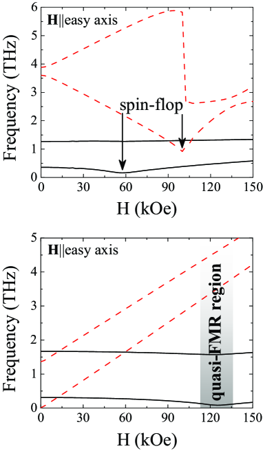
Figure 4: (Color online) Field dependencies of AFMR frequencies in LaTiO₃ (up) and YTiO₃ (bottom). $\bf H$ is parallel to c for LaTiO₃ and b for YTiO₃ (Pnma). These directions are close to easy axes. Curves are black for static orbital order and dashed red for orbital liquid.

Unfortunately, no any attention was paid to such powerful and sensitive method of magnetic structure and magnetic couplings investigation as antiferromagnetic/ferromagnetic resonance so far. The only attempt to observe electron spin resonance (ESR) below the magnetic transition temperatures (this is AFMR or FMR) and above them (EPR) was made by S. Okubo et al. Okubo et al. (1998) But, firstly, the AFMR signals for LaTiO₃ were not obtained at all, that might be because of frequency limits of the equipment used. And, secondly, this investigation was made only for powder samples and thus all direction-dependent effects were wiped out. We can’t but mention that if powder samples are used one neither will observe such an interesting field spectra as represented in Fig. 4, nor the strong orbital state dependence of these spectra can be obtained.

Finally, we argue that up-to-day, magnetic resonance is the ultimate method for distinguishing between static orbital order and orbital liquid. This method is a referee between opposite orbital states. Particularly, AFMR/FMR experiments with single crystals should put a dot at the end of the discussion what is the real orbital ground state in titanates — the remarkable system with strong entanglement of lattice, spin and orbital degrees of freedom.

We thank I.V. Solovyev for fruitful discussions. This work was partially supported by the ”Dynasty” foundation, by the CRDF REC-005, by the Russian Federal Scientific Program ”The development of scientific potential of the high school” and by the RFBR grant no. 08-02-00200.

References

- Imada et al. (1998) M. Imada, A. Fujimori, and Y. Tokura, Rev. Mod. Phys. 70, 1039 (1998).
- Khaliullin and Maekawa (2000) G. Khaliullin and S. Maekawa, Phys. Rev. Lett. 85, 3950 (2000).
- Khaliullin and Okamoto (2003) G. Khaliullin and S. Okamoto, Phys. Rev. B 68, 205109 (2003).
- Oleś et al. (2005) A. M. Oleś, G. Khaliullin, P. Horsch, and L. F. Feiner, Phys. Rev. B 72, 214431 (2005).
- Komarek et al. (2007) A. C. Komarek, H. Roth, M. Cwik, W.-D. Stein, J. B. M. Kriener, F. Bourée, T. Lorenz, and M. Braden, Phys. Rev. B 75, 224402 (2007).
- Cwik et al. (2003) M. Cwik, T. Lorenz, J. Baier, R. Müller, G. André, F. Bourée, F. Lichtenberg, A. Freimuth, R. Schmitz, E. Müller-Hartmann, et al., Phys. Rev. B 68, 060401 (2003).
- Mochizuki and M.Imada (2003) M. Mochizuki and M.Imada, Phys. Rev. Lett. 91, 167203 (2003).
- Mochizuki and M.Imada (2004) M. Mochizuki and M.Imada, New J. Phys. 6, 154 (2004).
- Kugel and Khomskii (1982) K. I. Kugel and D. I. Khomskii, Usp. Fiz. Nauk 25, 231 (1982).
- Meijer et al. (1999) G. I. Meijer, W. Henggeler, J. Brown, O.-S. Becker, J. G. Bednorz, C. Rossel, and P. Wachter, Phys. Rev. B 59, 11832 (1999).
- Ulrich et al. (2002) C. Ulrich, G. Khaliullin, S. Okamoto, M. Reehuis, A. Ivanov, H. He, Y. Taguchi, Y. Tokura, and B. Keimer, Phys. Rev. Lett. 89, 167202 (2002).
- Keimer et al. (2000) B. Keimer, D. Casa, A. Ivanov, J. W. Lynn, M. v. Zimmermann, J. P. Hill, D. Gibbs, Y. Taguchi, and Y. Tokura, Phys. Rev. Lett. 85, 3946 (2000).
- Kiyama and Itoh (2003) T. Kiyama and M. Itoh, Phys. Rev. Lett. 91, 167202 (2003).
- Haverkort et al. (2005) M. V. Haverkort, Z. Hu, A. Tanaka, G. Ghiringhelli, H. Roth, M. Cwik, T. Lorenz, C. Schüßler-Langeheine, S. V. Streltsov, A. S. Mylnikova, et al., Phys. Rev. Lett. 94, 056401 (2005).
- Schmitz et al. (2005) R. Schmitz, O. Entin-Wohlman, A. Aharony, A. B. Harris, and E. Müller-Hartmann, Phys. Rev. B 71, 144412 (2005).
- (16) R. Schmitz, O. Entin-Wohlman, A. Aharony, and E. Müller-Hartmann, eprint cond-mat/0506328 (unpublished).
- Solovyev (2006) I. V. Solovyev, Phys. Rev. B 74, 054412 (2006).
- Streltsov et al. (2005) S. V. Streltsov, A. S. Mylnikova, A. O. Shorikov, Z. V. Pchelkina, D. I. Khomskii, and V. I. Anisimov, Phys. Rev. B 71, 245114 (2005).
- Ulrich et al. (2006) C. Ulrich, A. Gössling, M. Grüninger, M. Guennou, H. Roth, M. Cwik, T. Lorenz, G. Khaliullin, and B. Keimer, Phys. Rev. Lett. 97, 157401 (2006).
- Nikiforov et al. (1980) A. E. Nikiforov, S. Y. Shashkin, and A. I. Krotkii, Phys. Status Solidi (b) 98, 289 (1980).
- Schmidt et al. (1993) M. W. Schmidt, K. K. Baldridge, J. A. Boatz, S. T. Elbert, M. S. Gordon, J. J. Jensen, S. Koseki, N. Matsunaga, K. A. Nguyen, S. Su, et al., J. Comput. Chem. 14, 1347 (1993).
- Schmidt and Gordon (1998) M. W. Schmidt and M. S. Gordon, Annu. Rev. Phys. Chem. 49, 233 (1998).
- Moriya (1960) T. Moriya, Phys. Rev. 120, 91 (1960).
- Nikiforov et al. (1971) A. E. Nikiforov, V. Y. Mitrofanov, and A. N. Men, Phys. Status Solidi (b) 45, 65 (1971).
- Eremina et al. (2004) R. M. Eremina, M. V. Eremin, V. V. Iglamov, J. Hemberger, H.-A. K. von Nidda, F. Lichtenberg, and A. Loidl, Phys. Rev. B 70, 224428 (2004).
- Anderson (1959) P. W. Anderson, Phys. Rev. 115, 2 (1959).
- Moskvin and Bostrem (1977) A. S. Moskvin and I. G. Bostrem, Sov. Phys. Solid State 19, 1616 (1977).
- Shekhtman et al. (1992) L. Shekhtman, O. Entin-Wohlman, and A. Aharony, Phys. Rev. Lett. 69, 836 (1992).
- Solovyev et al. (2007) I. V. Solovyev, Z. V. Pchelkina, and V. I. Anisimov, Phys. Rev. B 75, 045110 (2007).
- Okubo et al. (1998) S. Okubo, S. Kimura, H. Ohta, and M. Itoh, J. Magn. Magn. Mater. 177-181, 1373 (1998).