Exact solution of the extended Hubbard model in the atomic limit on the Bethe Lattice

Abstract

We study the phase diagram at finite temperature of a system of Fermi particles on the sites of the Bethe lattice with coordination number $z$ and interacting through onsite $U$ and nearest-neighbor $V$ interactions. This is a physical realization of the extended Hubbard model in the atomic limit. By using the equations of motion method, we exactly solve the model. For an attractive intersite potential, we find, at half filling, a phase transition towards a broken particle-hole symmetry state. The critical temperature, as a function of the relevant parameters, has a re-entrant behavior as already observed in the equivalent spin-1 Ising model on the Bethe lattice.

I introduction

Recently, it has been shown mancini_0506 that a system of $q$ species of Fermi particles, localized on the sites of a Bravais lattice, is exactly solvable in any dimension by means of the equations of motion approach mancini_04 . This Fermi system is isomorphic to a spin-$q/2$ Ising model in an external magnetic field. As a consequence, spin systems can be studied within a new approach mancini_0506 . Exactly solvable means that it is always possible to find a complete set of eigenvalues and eigenoperators of the Hamiltonian, which closes the hierarchy of the equations of motion. Thus, one can get exact expressions for the relevant Green’s functions and correlation functions. One finds that these functions depend on a finite set of parameters to be self-consistently determined mancini_04 . It has been already shown how it is possible to fix such parameters by means of symmetry and algebra constraints in the case of one dimensional systems for $q=1,2,3$ mancini_05 , and in the case of the Bethe lattice with coordination number $z$ and $q=1$ mancini_06 .

In this paper, we shall address the case of $q=2$ species of Fermi particles on the sites of the Bethe lattice with coordination number $z$ and interacting through nearest-neighbors interaction $V$. By considering also an onsite interaction $U$, one has the extended Hubbard model in the atomic limit. We find that for an attractive nearest-neighbor interaction there is a transition from a phase where the particle-hole symmetry is preserved to a phase where this symmetry is broken. The relative variations of the two regions depend on the coordination number $z$. Furthermore, for $U/|V|>2$ the phase diagram exhibits a re-entrant behavior.

The plan of the paper is as follows: in Sec. II, we outline the equations of motion method for the extended Hubbard model in the atomic limit. In Sec. III, we compute the Green’s and correlation functions and find that they depend only on two parameters. As a result, in Sec. IV, we are able to get a set of self-consistent equations enabling us to fix these parameters in terms of which all the local properties of the system can be expressed. In Sec. V we shall determine the transition temperature as a function of the onsite interaction at half filling and analyze the phase diagram for a wide range of values of the parameters $T$, $U$ (in units of $\left|V\right|)$ and for different values of the coordination number $z$. In Appendix A we briefly discuss the equivalence between the extended Hubbard model in the atomic limit and the spin-1 Ising model on the Bethe lattice pawloski_06 ; katsura_79 . Finally, Sec. VI is devoted to our concluding remarks.

II The Hamiltonian and the equations of motion

The extended Hubbard Hamiltonian in the atomic limit is given by

$$H=-\mu\sum_{i}n(i)+U\sum_{i}D(i)+\frac{1}{2}V\sum_{i\neq j}\,n(i)n(j),$$ (1)

where $U$ and $V$ represent the onsite and the nearest-neighbor intersite interaction, respectively. $\mu$ is the chemical potential, $n(i)=n_{\uparrow}(i)+n_{\downarrow}(i)$ and $D(i)=n_{\uparrow}(i)n_{\downarrow}(i)$ are the density and double occupancy operators at site $i$, respectively. As usual, $n_{\sigma}(i)=c_{\sigma}^{\dagger}(i)c_{\sigma}(i)$ with $\sigma=\left\{{\uparrow,\downarrow}\right\}$ and $c_{\sigma}(i)$ ($c_{\sigma}^{\dagger}(i))$ is the fermionic annihilation (creation) operator of an electron of spin $\sigma$ at site $i$, satisfying canonical anti-commutation relations. In the following we shall use the spinor notation for all fermionic operators. For instance, $c^{\dagger}(i)=({c_{\uparrow}^{\dagger}(i)\,\,\,c_{\downarrow}^{\dagger}(i)})$. The sums in Eq. (1) run over the sites of a Bravais lattice. Here, we shall consider as Bravais lattice the Bethe lattice, which is an infinite Cayley tree consisting of a central site - which we denote by (0) - with $z$ nearest-neighbors forming the first shell. Each site of a shell is joined to $z-1$ nearest-neighbors to form the second shell, and so on to infinity. Thus, on the Bethe lattice, the Hamiltonian (1) may be conveniently written as

$$H=-\mu n(0)+UD(0)+\sum\limits_{p=1}^{z}H^{(p)},$$ (2)

where $H^{(p)}$ represents the Hamiltonian of the $p$-th sub-tree rooted at the central site (0) and it can be written as

$$H^{(p)}=-\mu n(p)+UD(p)+Vn(0)n(p)+\sum\limits_{m=1}^{z-1}H^{(p,m)},$$ (3)

where $p$ are the nearest-neighbors of the site (0). In turns, $H^{(p,m)}$ describes the $m$-th sub-tree rooted at the site $(p)$, and so on to infinity.

The density operator cannot be used to employ the standard methods based on the equations of motion since it does not depend on time. In order to use the Green’s function formalism one may consider the Hubbard operators $\xi(i)=[n(i)-1]c(i)$ and $\eta(i)=n(i)c(i)$, obeying to the following equations of motion:

$$\begin{split}i\frac{\partial}{\partial t}\xi(i)&=-\mu\xi(i)+zV\xi(i)n^{\alpha}(i)\\ i\frac{\partial}{\partial t}\eta(i)&=(U-\mu)\eta(i)+zV\eta(i)n^{\alpha}(i)\,\end{split}$$ (4)

where $n^{\alpha}(i)=\sum\nolimits_{p=1}^{z}n(i,p)/z$, and $(i,p)$ are the nearest neighbors of site $i$. The algebra satisfied by the operators $n$ and $D$ mancini_04 , allows one to establish an important recurrence relation obeyed by $n^{\alpha}(i)$:

$$[n^{\alpha}(i)]^{k}=\sum\limits_{m=1}^{2z}A_{m}^{(k)}[n^{\alpha}(i)]^{m},$$ (5)

where the coefficients $A_{m}^{(k)}$ are rational numbers which can be easily determined by the algebra and the structure of the Bethe lattice, and which satisfy the relations $\sum\nolimits_{m=1}^{2z}A_{m}^{(k)}=1$ and $A_{m}^{(k)}=\delta_{m,k}$ $(k=1,\cdots,2z)$ mancini_07 . The recurrence relation (5) is of seminal importance because it limits the number of composite operators which can be generated by the dynamics of the original fermionic operators. In fact, by taking successive time derivatives of the Hubbard operators $\xi(i)$ and $\eta(i)$, one clearly sees that for $k>2z$, no additional composite operators are generated and the equations of motion close mancini_0506 . Thus, one may define a new composite field operator $\psi(i)$ mancini_04 :

$$\psi(i)=\left({{\begin{array}[]{*{20}c}{\psi^{(\xi)}(i)}\\ {\psi^{(\eta)}(i)}\\ \end{array}}}\right);\quad\psi^{(\xi)}(i)=\left({{\begin{array}[]{*{20}c}{\psi_{1}^{(\xi)}(i)}\\ {\psi_{2}^{(\xi)}(i)}\\ \vdots\hfill\\ {\psi_{2z+1}^{(\xi)}(i)}\\ \end{array}}}\right)=\left({{\begin{array}[]{*{20}c}{\xi(i)\hfill}\\ {\xi(i)[n^{\alpha}(i)]}\\ \vdots\\ {\xi(i)[n^{\alpha}(i)]^{2z}}\\ \end{array}}}\right)\quad\psi^{(\eta)}(i)=\left({{\begin{array}[]{*{20}c}{\psi_{1}^{(\eta)}(i)}\\ {\psi_{2}^{(\eta)}(i)}\\ \vdots\\ {\psi_{2z+1}^{(\eta)}(i)}\\ \end{array}}}\right)=\left({{\begin{array}[]{*{20}c}{\eta(i)}\\ {\eta(i)[n^{\alpha}(i)]}\\ \vdots\\ {\eta(i)[n^{\alpha}(i)]^{2z}}\\ \end{array}}}\right).$$ (6)

By means of the recursion formula (5), the operators $\psi^{(\xi)}(i)$ and $\psi^{(\eta)}(i)$ satisfy the equations of motion:

$$\begin{split}i\frac{\partial}{\partial t}\psi^{(\xi)}(i)&=[\psi^{(\xi)}(i),H]=\varepsilon^{(\xi)}\psi^{(\xi)}(i)\\ i\frac{\partial}{\partial t}\psi^{(\eta)}(i)&=[\psi^{(\eta)}(i),H]=\varepsilon^{(\eta)}\psi^{(\eta)}(i)\end{split}$$ (7)

where $\varepsilon^{(\xi)}$ and $\varepsilon^{(\eta)}$ are the energy matrices of rank $(2z+1)\times(2z+1)$:

$$\varepsilon^{(\xi)}=\left({{\begin{array}[]{*{20}c}{-\mu}&{zV}&0\hfill&\cdots&0&0&0\\ 0&{-\mu}&{zV}&\cdots&0&0&0\\ 0&0&{-\mu}&\cdots&0&0&0\\ \vdots&\vdots&\vdots&\cdots&\vdots&\vdots&\vdots\\ 0&0&0&\cdots&{-\mu}&{zV}&0\\ 0&0&0&\cdots&0&{-\mu}&{zV}\\ 0&{zVA_{1}^{(2z+1)}}&{zVA_{2}^{(2z+1)}}&\cdots&{zVA_{2z-2}^{(2z+1)}}&{zVA_{2z-1}^{(2z+1)}}&{-\mu+zVA_{2z}^{(2z+1)}}\\ \end{array}}}\right)$$ (8)

$$\varepsilon^{(\eta)}=\left({{\begin{array}[]{*{20}c}{U-\mu}&{zV}&0&\cdots&0&0&0\\ 0&{U-\mu}&{zV}&\cdots&0&0&0\\ 0&0&{U-\mu}&\cdots&0&0&0\\ \vdots&\vdots&\vdots&\cdots&\vdots&\vdots&\vdots\\ 0&0&0&\cdots&{U-\mu}&{zV}&0\\ 0&0&0&\cdots&0&{U-\mu}&{zV}\\ 0&{zVA_{1}^{(2z+1)}}&{zVA_{2}^{(2z+1)}}&\cdots&{zVA_{2z-2}^{(2z+1)}}&{zVA_{2z-1}^{(2z+1)}}&{U-\mu+zVA_{2z}^{(2z+1)}}\\ \end{array}}}\right)$$ (9)

whose eigenvalues, $E_{m}^{(\xi)}$ and $E_{m}^{(\eta)}$, are given by:

$$\begin{split}E_{m}^{(\xi)}&=-\mu+(m-1)V\\ E_{m}^{(\eta)}&=-\mu+U+(m-1)V,\end{split}$$ (10)

where $m=1,...,(2z+1)$. It is easy to convince oneself that the Hamiltonian (2) has now been formally solved since one has a closed set of eigenoperators and eigenvalues. Then, by using the formalism of Green’s functions (GF), one can proceed to the calculation of observable quantities.

The two field operators $\psi^{(\xi)}(i)$ and $\psi^{(\eta)}(i)$ are decoupled at the level of equations of motion, as one may clearly see in Eq. (7). However, as we shall see in the next Sections, they are coupled via a set of self-consistent equations allowing for the determination of some unknown parameters in terms of which observables quantities may be computed.

III Retarded Green’s function and correlation functions

The retarded thermal Green’s function is defined as:

$$G^{(s)}(t-{t}^{\prime})=\langle{R\,\left[{\psi^{(s)}(0,t)\,{\psi^{(s)}}^{\dagger}(0,{t}^{\prime})}\right]}\rangle=\theta(t-{t}^{\prime})\langle{\left\{{\psi^{(s)}(0,t),{\psi^{(s)}}^{\dagger}(0,{t}^{\prime})}\right\}}\rangle,$$ (11)

where the index $s$ refers either to the Hubbard operator $\xi$ or $\eta$ and $\langle\cdots\rangle$ denotes the quantum-statistical average over the grand canonical ensemble. By means of the field equations (6), one finds that the retarded GF satisfies the equation

$$\left[{\omega-\varepsilon^{(s)}}\right]G^{(s)}(\omega)=I^{(s)},$$ (12)

where $G^{(s)}(\omega)$ is the Fourier transform of $G^{\left(s\right)}(t-{t}^{\prime})$ and $I^{(s)}=\langle{\left\{{\psi^{(s)}(0,t),{\psi^{(s)}}^{\dagger}(0,t)}\right\}}\rangle$ is the $(2z+1)\times(2z+1)$ normalization matrix. The solution of Eq. (12) is mancini_04 :

$$G^{(s)}(\omega)=\sum_{m=1}^{2z+1}\frac{\sigma^{(s,m)}}{\omega-E_{m}^{(s)}+i\delta},$$ (13)

where $E_{m}^{(s)}$ are the eigenvalues of the energy matrices, as given in Eq. (10). The spectral density matrices $\sigma_{ab}^{(s,n)}$ can be computed by means of the formula mancini_04 :

$$\sigma_{ab}^{(s,n)}=\Omega_{an}^{(s)}\sum\limits_{c=1}^{2z+1}\left[{\Omega_{nc}^{(s)}}\right]^{-1}I_{cb}^{(s)}.$$ (14)

In Eq. (14), $\Omega^{(s)}$ is the $(2z+1)\times(2z+1)$ matrix whose columns are the eigenvectors of the energy matrix $\varepsilon^{(s)}$. It is straightforward to show that $\Omega^{(\xi)}=\Omega^{(\eta)}=\Omega$, where the matrix $\Omega$ is given by:

$$\Omega_{p,k}=\left\{\begin{array}[]{cl}1&\quad\quad k=1,\;p=1\\ 0&\quad\quad k=1,\;p\neq 1\\ (\frac{z}{k-1})^{2z+1-p}&\quad\quad k\neq 1\,.\end{array}\right.$$ (15)

Moreover, the matrix elements of the normalization matrices in Eq. (14) can be cast in a simple form as mancini_05

$$\begin{split}I_{n,m}^{(\xi)}&=\kappa^{(n+m-2)}-\lambda^{(n+m-2)}\\ I_{n,m}^{(\eta)}&=\lambda^{(n+m-2)},\ \end{split}$$ (16)

where the charge correlators $\kappa^{(k)}$ and $\lambda^{(k)}$ are defined as

$$\begin{split}\kappa^{(k)}&=\langle{[n^{\alpha}(0)]^{k}}\rangle\\ \lambda^{(k)}&=\frac{1}{2}\langle{n(0)[n^{\alpha}(0)]^{k}}\rangle.\end{split}$$ (17)

Similarly, one finds that the correlation function (CF)

$$C^{(s)}(t-{t}^{\prime})=\langle{\psi^{(s)}(0,t)\,{\psi^{(s)}}^{\dagger}(0,{t}^{\prime})}\rangle=\frac{1}{(2\pi)}\int\limits_{-\infty}^{+\infty}d\omega\,{\kern 1.0pt}e^{-i\omega(t-{t}^{\prime})}C^{(s)}(\omega)\,,$$ (18)

can also be expressed in terms of the same charge correlators (17). In fact, by means of the relation mancini_06 :

$$C(\omega)=-\left[{1+\tanh\frac{\beta\omega}{2}}\right]\,Im\left[{G(\omega)}\right],$$ (19)

where $\beta=1/k_{B}T$, the CF can be immediately computed from Eq. (13). One obtains

$$\begin{split}C^{(s)}(\omega)&=\pi\,\sum\limits_{m=1}^{2z+1}\sigma^{(s,n)}T_{m}^{(s)}\,\delta\left({\omega-E_{m}^{(s)}}\right)\\ C^{(s)}(t-{t}^{\prime})&=\frac{1}{2}{\kern 1.0pt}\,\sum\limits_{m=1}^{2z+1}e^{-iE_{m}^{(s)}(t-{t}^{\prime})}\,\sigma^{(s,n)}\,T_{m}^{(s)},\end{split}$$ (20)

where $T_{m}^{(s)}=1+\tanh({\beta E_{m}^{(s)}/2})$. As one can clearly see, the knowledge of the GF’s and, consequently of the CF’s, is not fully achieved. In fact, they depend on the unknown correlators $\kappa^{(k)}$ and $\lambda^{(k)}$which are expectation values of operators not belonging to the basis (6). In the next Section we shall show how these quantities can be self-consistently computed.

IV Self-consistent equations

In order to compute the unknown correlators (17), one may start by noticing that, by exploiting the recursion relation (5), also $\kappa^{(k)}$ and $\lambda^{(k)}$ obey to a recursion relation which limits their computation just to the first $2z$ correlators mancini_07 :

$$\begin{split}\kappa^{(k)}&=\sum\limits_{m=1}^{2z}A_{m}^{(k)}\kappa^{(m)}\\ \lambda^{(k)}&=\sum\limits_{m=1}^{2z}A_{m}^{(k)}\lambda^{(m)}.\end{split}$$ (21)

Then, one may split the Hamiltonian (4) as the sum of two terms:

$$\begin{split}H&=H_{0}+H_{I}\\ H_{I}&=zVn(0)n^{\alpha}(0).\end{split}$$ (22)

Since $H_{0}$ and $H_{I}$ commute, the quantum statistical average of a generic operator $O$ can be expressed as:

$$\langle O\rangle=\frac{Tr\{Oe^{-\beta H}\}}{Tr\{e^{-\beta H}\}}=\frac{\langle{O\,e^{-\beta H_{I}}}\rangle_{0}}{\langle{e^{-\beta H_{I}}}\rangle_{0}},$$ (23)

where $\langle\cdots\rangle_{0}$ stands for the trace with respect to the reduced Hamiltonian $H_{0}$. One then considers the correlation functions

$$C_{1,k}^{(s)}=\langle{s(0)s^{\dagger}(0)\left[{n^{\alpha}\left(0\right)}\right]^{k-1}}\rangle,\quad s=\xi,\eta,\quad k=1,...,2z+1\,,$$ (24)

which, by means of Eq. (23), can be written as:

$$C_{1,k}^{(s)}=\frac{\langle s(0)s^{\dagger}(0)\left[n^{\alpha}(0)\right]^{k-1}e^{-\beta H_{I}}\rangle_{0}}{\langle e^{-\beta H_{I}}\rangle_{0}},\quad s=\xi,\eta,\quad k=1,...,2z+1\,.$$ (25)

The Pauli principle leads to the following algebraic relations

$$\begin{split}\xi^{\dagger}(i)n(i)&=0\\ \xi^{\dagger}(i)D(i)&=0\end{split}\quad\quad\quad\begin{split}\eta^{\dagger}(i)n(i)&=\eta^{\dagger}(i)\\ \eta^{\dagger}(i)D(i)&=0\end{split}$$ (26)

from which one has $\xi^{\dagger}(0)\,e^{-\beta H_{I}}=\xi^{\dagger}(0)$ and $\eta^{\dagger}(0)\,e^{-\beta H_{I}}=\eta^{\dagger}(0)\,e^{-z\beta Vn^{\alpha}(0)}$. The Hamiltonian $H_{0}$ describes a system where the original lattice has been reduced to the central site (0) and to $z$ unconnected sublattices. Thus, in the $H_{0}$-representation, the correlation functions connecting sites belonging to disconnected graphs can be decoupled. As a result, Eqs. (25) can be rewritten as:

$$C_{1,k}^{(\xi)}=\frac{\langle{\xi(0)\xi^{\dagger}(0)}\rangle_{0}\langle{[n^{\alpha}(0)]^{k-1}}\rangle_{0}}{\langle{e^{-\beta H_{I}}}\rangle_{0}},\quad\quad C_{1,k}^{(\eta)}=\frac{\langle{\eta(0)\eta^{\dagger}(0)}\rangle_{0}\langle{[n^{\alpha}(0)]^{k-1}e^{-z\beta Vn^{\alpha}(0)}}\rangle_{0}}{\langle{e^{-\beta H_{I}}}\rangle_{0}}\,.$$ (27)

In the $H_{0}$-representation, the Hubbard operators obey to simple equations of motion: $[\xi(i),H_{0}]=-\mu\,\xi(i)$ and $[\eta(i),H_{0}]=-(\mu-U)\,\eta(i)$. Thus, it is easy to show that the equal time CF’s can be expressed as:

$$\begin{split}\langle{\xi(0)\xi^{\dagger}(0)}\rangle_{0}&=\frac{1}{1+2e^{\beta\mu}+e^{\beta(2\mu-U)}}=1-B_{1}+B_{2}\\ \langle{\eta(0)\eta^{\dagger}(0)}\rangle_{0}&=\frac{e^{\beta\mu}}{1+2e^{\beta\mu}+e^{\beta(2\mu-U)}}=\frac{1}{2}(B_{1}-2B_{2}),\end{split}$$ (28)

where:

$$\begin{split}B_{1}&=\langle{n(0)}\rangle_{0}=\frac{2e^{\beta\mu}(1+e^{\beta(\mu-U)})}{1+2e^{\beta\mu}+e^{\beta(2\mu-U)}}\\ B_{2}&=\langle{D(0)}\rangle_{0}=\frac{e^{\beta(2\mu-U)}}{1+2e^{\beta\mu}+e^{\beta(2\mu-U)}}\,\end{split}$$ (29)

and one has used the identities

$$\xi_{\sigma}\xi_{\sigma}^{\dagger}+\eta_{\sigma}\eta_{\sigma}^{\dagger}=1-n_{\sigma},\quad\eta_{\sigma}\eta_{\sigma}^{\dagger}=n_{\sigma}-n_{\uparrow}n_{\downarrow}.$$ (30)

Upon inserting Eqs. (28) into Eqs. (27) and by taking $k=1$, one finds:

$$\begin{split}C_{1,1}^{(\xi)}&=\frac{1-B_{1}+B_{2}}{\langle e^{-\beta H_{I}}\rangle_{0}}\\ C_{1,1}^{(\eta)}&=\frac{\left({B_{1}-2B_{2}}\right)\langle e^{-z\beta Vn^{\alpha}(0)}\rangle_{0}}{2\langle e^{-\beta H_{I}}\rangle_{0}}.\end{split}$$ (31)

It is not difficult to show that the averages in the above equations can be expressed as:

$$\begin{split}\langle{e^{-\beta H_{I}}}\rangle_{0}&=1-B_{1}+B_{2}+(B_{1}-2B_{2})(1+aX_{1}+a^{2}X_{2})^{z}+B_{2}(1+dX_{1}+d^{2}X_{2})^{z}\\ \langle{e^{-z\beta Vn^{\alpha}(0)}}\rangle_{0}&=(1+aX_{1}+a^{2}X_{2})^{z},\end{split}$$ (32)

where $K=e^{-\beta V}$, $a=(K-1)$, $d=(K^{2}-1)$. $X_{1}$ and $X_{2}$ are two parameters defined as:

$$X_{1}=\langle{n^{\alpha}}\rangle_{0},\quad\quad X_{2}=\langle{D^{\alpha}}\rangle_{0}.$$ (33)

$X_{1}$ and $X_{2}$ are parameters of seminal importance since all correlators and fundamental properties of the system under study can be expressed in terms of them. Relevant physical quantities, such as the mean value of the particle density and doubly occupancy, and the charge correlators $\kappa^{(k)}$ and $\lambda^{(k)}$ can be easily computed mancini_07 :

$$\begin{split}n&=\frac{(X_{1}-2X_{2})(1+aX_{1}+a^{2}X_{2})+2X_{2}(1+dX_{1}+d^{2}X_{2})}{(1-X_{1}+X_{2})+(X_{1}-2X_{2})(1+aX_{1}+a^{2}X_{2})+X_{2}(1+dX_{1}+d^{2}X_{2})}\\ D&=\frac{X_{2}(1+dX_{1}+d^{2}X_{2})}{(1-X_{1}+X_{2})+(X_{1}-2X_{2})(1+aX_{1}+a^{2}X_{2})+X_{2}(1+dX_{1}+d^{2}X_{2})},\end{split}$$ (34)

and

$$\begin{split}\kappa^{(k)}&=\frac{1}{\langle{e^{-\beta H_{I}}}\rangle_{0}}\left\{{\langle{[n^{\alpha}(0)]^{k}}\rangle_{0}+\sum\limits_{m=1}^{2z}(B_{1}f_{m}^{(z)}+B_{2}g_{m}^{(z)})\langle{[n^{\alpha}(0)]^{m+k}}\rangle_{0}}\right\}\\ \lambda^{(k)}&=\frac{1}{2\langle{e^{-\beta H_{I}}}\rangle_{0}}\left\{{B_{1}\langle{[n^{\alpha}(0)]^{k}}\rangle_{0}+\sum\limits_{m=1}^{2z}[(B_{1}+2B_{2})f_{m}^{(z)}+2B_{2}g_{m}^{(z)}]\langle{[n^{\alpha}(0)]^{m+k}}\rangle_{0}}\right\},\end{split}$$ (35)

where $f_{m}^{(z)}$ and $g_{m}^{(z)}$ are some easily computable coefficients depending on the external parameters $T$ and $V$ and where the expectation value $\langle{[n^{\alpha}(0)]^{k}}\rangle_{0}$ can also be expressed in terms of $X_{1}$ and $X_{2}$ mancini_07 .

As a result, the solution of the model has been reduced to the determination of just two parameters. $X_{1}$ and $X_{2}$ can be determined by imposing translational invariance. In particular, the requests $\langle{n(0)}\rangle=\langle{n^{\alpha}(0)}\rangle$ and $\langle{D(0)}\rangle=\langle{D^{\alpha}(0)}\rangle$ lead to a set of two self-consistent equations mancini_07 :

$$\begin{split}X_{1}&=2e^{\beta\mu}(1-X_{1}-dX_{2})(1+aX_{1}+a^{2}X_{2})^{z-1}+e^{\beta(2\mu-U)}[2+(d-1)X_{1}-2dX_{2}](1+dX_{1}+d^{2}X_{2})^{z-1}\\ X_{2}&=e^{\beta(2\mu-U)}[1+dX_{1}-(2d+1)X_{2}](1+dX_{1}+d^{2}X_{2})^{z-1}-2e^{\beta\mu}K^{2}X_{2}(1+aX_{1}+a^{2}X_{2})^{z-1}.\end{split}$$ (36)

A full investigation of these equations will be given elsewhere. In this communication, we shall restrict our analysis to the possibility of a breakdown of the particle-hole symmetry.

V Breakdown of the particle-hole symmetry

In this Section we shall study the possibility of a spontaneous breaking of the particle-hole symmetry. Let us consider the following value of the chemical potential: $\mu=U/2+zV$. For this value of $\mu$, Eqs. (36) become

$$X_{1} = 2GK^{-z}(1-X_{1}-dX_{2})(1+aX_{1}+a^{2}X_{2})^{z-1}+K^{-2z}[2+(d-1)X_{1}-2dX_{2}](1+dX_{1}+d^{2}X_{2})^{z-1}$$ (37)

$$X_{2} = K^{-2z}[1+dX_{1}-(2d+1)X_{2}](1+dX_{1}+d^{2}X_{2})^{z-1}-2GK^{-z+2}X_{2}(1+aX_{1}+a^{2}X_{2})^{z-1},$$ (38)

and Eqs. (34) become:

$$\begin{split}n&=\frac{2GK^{z}(1+aX_{1}+a^{2}X_{2})^{z}+2(1+dX_{1}+d^{2}X_{2})^{z}}{K^{2z}+2GK^{z}(1+aX_{1}+a^{2}X_{2})^{z}+(1+dX_{1}+d^{2}X_{2})^{z}}\\ D&=\frac{(1+dX_{1}+d^{2}X_{2})^{z}}{K^{2z}+2GK^{z}(1+aX_{1}+a^{2}X_{2})^{z}+(1+dX_{1}+d^{2}X_{2})^{z}},\end{split}$$ (39)

where $G=e^{\beta U/2}$. It is easy to show that for

$$X_{1}=1-dX_{2}\,$$ (40)

Eq. (37) is always satisfied. Then, by substituting Eq. (40) into Eq. (39) one obtains

$$n=1,\quad\quad D=\frac{1}{2+2G(1-a^{2}X_{2})^{z}}.$$ (41)

That is, solution (40) is in agreement with the particle-hole symmetry. Upon inserting Eq. (40) into Eq. (38) one obtains:

$$X_{2}(1+K^{2})+2GKX_{2}(1-a^{2}X_{2})^{z-1}-1=0.$$ (42)

Thus, for $\mu=U/2+zV$, Eqs. (36) admit a solution which satisfies the particle-hole symmetry and is described by the set of equations (40) and (42). One may ask oneself if Eqs. (37) and (38) do admit other solutions, different from the one described by (40) and (42) and thus breaking the particle-hole symmetry. To this purpose, one may perturb the solution (40), by setting $X_{1}=1-dX_{2}+w$. With a little algebra it is easy to show that a solution with $w\neq 0$ does exist if, and only if, the following equation

$$2K^{\frac{U/\left|V\right|+2}{2}}[z+K(z-2)]^{z-1}+(K+1)^{z-1}(z-1)^{z-1}[z-K^{2}(z-2)]=0$$ (43)

is satisfied. This equation will fix the critical temperature $T_{c}$ below which the system admits other solutions, which do not satisfy the particle-hole symmetry. Numerical calculations show that Eq. (43) admits a solution only for negative values of $V$. Thus, in the following, we shall consider only the case of attractive intersite potential. It is interesting to consider Eq. (43) in two extremal limits, namely $U/\left|V\right|\to-\infty$ and $T_{c}\to 0$. In the former limit, as expected, one finds that the critical temperature is the same as the one of a spinless fermionic system on the Bethe lattice, equivalent to the spin-1/2 Ising model mancini_06 ; mancini_07 ; baxter_82 :

$$z-K^{2}(z-2)=0\quad\quad\Rightarrow\quad\quad K_{c}^{2}=\frac{z}{z-2}\quad\quad\Rightarrow\quad\quad\frac{k_{B}T_{c}}{\left|V\right|}=\frac{2}{\ln\left({\frac{z}{z-2}}\right)}.$$ (44)

The limit $T_{c}\to 0$ provides the value of the ratio $U/|V|$ at which one should expect a quantum phase transition:

$$2e^{\beta U/2}(z-2)^{z-1}-(z-1)^{z-1}K(z-2)=0\quad\Rightarrow\quad\left({U/2-\left|V\right|}\right)=k_{B}T_{c}\ln\left[{\frac{(z-1)^{z-1}}{2(z-2)^{z-2}}}\right].$$ (45)

Thus, in the limit $T_{c}\to 0$, one finds that $U/|V|=2$, independently of the value of $z$. The results obtained from Eq. (43) are displayed in Fig. 1. One observes that, at fixed coordination number, by increasing $U$ from large negative values (i.e., attractive onsite interaction) one finds a decrease of the critical temperature.

An interesting feature of the model’s phase diagram is that it shows regimes with a re-entrance: namely, fixing $U/|V|>2$ and lowering the temperature, one switches from a particle-hole symmetry preserving phase to another one where this symmetry is broken at a certain critical temperature. Then, as evidenced in Fig. 1, lowering further the temperature, one finds another critical temperature at which the symmetry is restored. How pronounced the re-entrance is, depends on $z$.

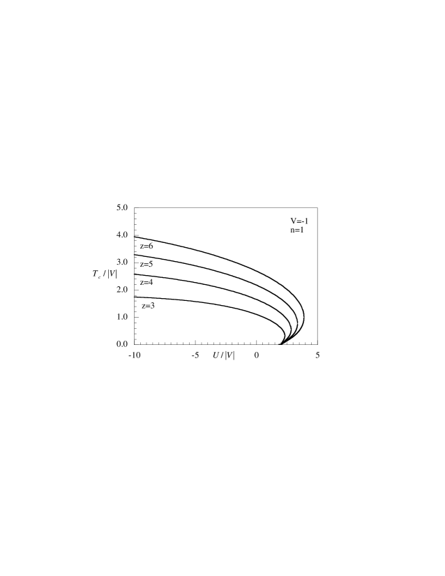
Figure 1: The normalized critical temperature $T_{c}/|V|$ as a function of the on site interaction $U/|V|$ for different values of the coordination number $z$ of the Bethe lattice.

VI Concluding Remarks

In this paper we have obtained the finite temperature phase diagram of a system of fermions with onsite and nearest-neighbor interactions localized on the sites of the Bethe lattice. The Hamiltonian describing such a system defines the so-called extended Hubbard model in the atomic limit. Upon using the equations of motion method, it is possible to exactly solve the model. For attractive nearest-neighbor interaction we find the critical temperature at which the system undergoes a transition to a phase where the particle-hole symmetry is broken. This critical temperature depends on the ratio $U/|V|$ and on $z$. It increases with increasing $z$ and presents a re-entrant behavior for $U/|V|>2$.

Appendix A Spin-1 Ising model on the Bethe lattice

In this Appendix we shall analyze the correspondence between the extended Hubbard model on the Bethe lattice and the spin-1 Ising model defined on the same lattice. A transformation from a fermionic to a spin Hamiltonian can be performed by the use of the pseudospin variable $S(i)$:

$$S(i)=n_{\uparrow}(i)+n_{\downarrow}(i)-1=n(i)-1.$$ (46)

$S(i)$ can take four values, with $S(i)$=0 double degenerate:

$$\begin{split}n_{\uparrow}(i)&=0\quad\quad\\ n_{\uparrow}(i)&=1\quad\quad\\ n_{\uparrow}(i)&=0\quad\quad\\ n_{\uparrow}(i)&=1\quad\quad\end{split}\begin{split}n_{\downarrow}(i)&=0\quad\quad\Leftrightarrow\\ n_{\downarrow}(i)&=0\quad\quad\Leftrightarrow\\ n_{\downarrow}(i)&=1\quad\quad\Leftrightarrow\\ n_{\downarrow}(i)&=1\quad\quad\Leftrightarrow\\ \end{split}\begin{split}\quad\quad S(i)&=-1\\ \quad\quad S(i)&=0\\ \quad\quad S(i)&=0\\ \quad\quad S(i)&=1\end{split}$$ (47)

Under the transformation (46) the Hamiltonian (2) can be cast in the form:

$$\begin{split}H&=\Delta\,S^{2}(0)-h\,S(0)+E_{0}+\sum\limits_{p=1}^{z}H^{(p)}\\ H^{(p)}&=-J\,S(0)S(p)+\Delta\,\,S^{2}(p)-h\,S(p)+\sum\limits_{m=1}^{z-1}H^{(p,m)},\end{split}$$ (48)

where $E_{0}=-V+(-\mu+V)N$, $N$ is the total number of sites, $h=\mu-zV-U/2$, $J=-V$ and $\Delta=U/2$. Thus, the Hamiltonian (48) appears as the one of a spin-1 Ising model with nearest-neighbor exchange interaction $J$ in the presence of a crystal field $\Delta$ and of an external magnetic field $h$. The difference here is that the Hamiltonian (48) is pertinent to a four-level system because of the spin degeneracy. It is possible to get rid of the spin degeneracy by mapping the fermionic Hamiltonian on the standard spin-1 Ising one with $\tilde{S}(i)=\left\{{-1,0,1}\right\}$ paying the price of making the crystal field $\Delta$ to be temperature dependent micnas_84 ; pawloski_06 : $\tilde{\Delta}=U/2+k_{B}T\log 2$. The double degeneracy of every $S(i)=0$ leads to a factor 2 for every singly occupied site in the partition function of the classical spin system. This gives rise to an overall factor

$$\prod_{i}2^{1-\tilde{S}^{2}(i)}=2^{\sum_{i}[1-\tilde{S}^{2}(i)]}$$ (49)

One may rewrite the partition function of Hamiltonian (48) as follows:

$$Z=\sum_{\{S(i)\}=\{-1,0,0,1\}}\exp\{-\beta H[S(i)]\}=\sum_{\{\tilde{S}(i)\}=\{-1,0,0,1\}}\exp\{-\beta\tilde{H}[\tilde{S}(i)]\}$$ (50)

where $\tilde{H}$ is the Hamiltonian of the standard spin-1 Ising model on the Bethe lattice, but now with an effective temperature-dependent crystal field:

$$\begin{split}\tilde{H}&=\tilde{\Delta}\,\tilde{S}^{2}(0)-h\,\tilde{S}(0)+\tilde{E}_{0}+\sum_{p=1}^{z}\tilde{H}^{(p)}\\ \tilde{H}^{(p)}&=-J\,\tilde{S}(0)\tilde{S}(p)+\tilde{\Delta}\,\,\tilde{S}^{2}(p)-h\,\tilde{S}(p)+\sum_{m=1}^{z-1}\tilde{H}^{(p,m)}\\ \end{split}$$ (51)

where $\tilde{E}_{0}=E_{0}+k_{B}T\ln 2$ and $\tilde{\Delta}=\Delta+k_{B}T\,\ln 2$. Having established the mapping between the two models, we find that our critical temperature exactly agrees with the one previously found in the literature katsura_79 .

References

- (1) F. Mancini, Europhys. Lett. 70, 485 (2005); Cond. Matt. Phys. 9, 393 (2006).
- (2) F. Mancini and A. Avella, Adv. Phys. 53, 537 (2004).
- (3) F. Mancini, Eur. Phys. J. B 45, 497 (2005); Eur. Phys. J. B 47, 527 (2005); A. Avella and F. Mancini, Eur. Phys. J. B 50, 527 (2006).
- (4) F. Mancini and A. Naddeo, Phys. Rev. E 74, 061108 (2006); Physica C (2007) in print.
- (5) F. Mancini, F. P. Mancini and A. Naddeo, in preparation.
- (6) R. J. Baxter, Exactly Solvable Models in Statistical Mechanics, Academic Press, New York (1982).
- (7) R. Micnas, S. Robaszkiewicz and K. A. Chao, Phys. Rev. B 29, 2784 (1984).
- (8) G. Pawłowski, Eur. Phys. J. B 53, 471 (2006).
- (9) S. Katsura, J. Phys. A 12, 2087 (1979); K. G. Chakraborty and J. W. Tucker, Phys. A 137, 122 (1986).