Recent developments in effective field theory

Abstract

We will give a short introduction to the one-nucleon sector of chiral perturbation theory and will address the issue of a consistent power counting and renormalization. We will discuss the infrared regularization and the extended on-mass-shell scheme. Both allow for the inclusion of further degrees of freedom beyond pions and nucleons and the application to higher-loop calculations. As applications we consider the chiral expansion of the nucleon mass to order ${\cal O}(q^{6})$ and the inclusion of vector and axial-vector mesons in the calculation of nucleon form factors.

1 Introduction

Effective field theory (EFT) has become a powerful tool in the description of the strong interactions at low energies. The central idea is due to Weinberg [1]:

”… if one writes down the most general possible Lagrangian, including all terms consistent with assumed symmetry principles, and then calculates matrix elements with this Lagrangian to any given order of perturbation theory, the result will simply be the most general possible S–matrix consistent with analyticity, perturbative unitarity, cluster decomposition and the assumed symmetry principles.”

The prerequisite for an effective field theory program is (a) a knowledge of the most general effective Lagrangian and (b) an expansion scheme for observables in terms of a consistent power counting method. The application of these ideas to the interactions among the Goldstone bosons of spontaneous chiral symmetry breaking in QCD results in mesonic chiral perturbation theory (ChPT) [1, 2] (see, e.g., Refs. [3, 4, 5, 6] for an introduction and overview). In the following we will outline some recent developments in devising a renormalization scheme leading to a simple and consistent power counting for the renormalized diagrams of a manifestly Lorentz-invariant approach to baryon ChPT [7].

2 Renormalization and Power Counting

2.1 Effective Lagrangian and Power Counting

The effective Lagrangian relevant to the one-nucleon sector consists of the sum of the purely mesonic and $\pi N$ Lagrangians, respectively,

$${\cal L}_{\rm eff}={\cal L}_{\pi}+{\cal L}_{\pi N}={\cal L}_{\pi}^{(2)}+{\cal L}_{\pi}^{(4)}+\cdots+{\cal L}_{\pi N}^{(1)}+{\cal L}_{\pi N}^{(2)}+\cdots,$$

which are organized in a derivative and quark-mass expansion [1, 2, 7]. For example, the lowest-order basic Lagrangian ${\cal L}_{\pi N}^{(1)}$, already expressed in terms of renormalized parameters and fields, is given by

$${\cal L}_{\pi N}^{(1)}=\bar{\Psi}\left(i\gamma_{\mu}\partial^{\mu}-m\right)\Psi-\frac{1}{2}\frac{\texttt{g}_{A}}{F}\bar{\Psi}\gamma_{\mu}\gamma_{5}\tau^{a}\partial^{\mu}\pi^{a}\Psi+\cdots,$$ (1)

where $m$, $\texttt{g}_{A}$, and $F$ denote the chiral limit of the physical nucleon mass, the axial-vector coupling constant, and the pion-decay constant, respectively. The ellipsis refers to terms containing external fields and higher powers of the pion fields. When studying higher orders in perturbation theory one encounters ultraviolet divergences. As a preliminary step, the loop integrals are regularized, typically by means of dimensional regularization. For example, the simplest dimensionally regularized integral relevant to ChPT is given by

$$I(M^{2},\mu^{2},n) = \mu^{4-n}\int\frac{\mbox{d}^{n}k}{(2\pi)^{n}}\frac{i}{k^{2}-M^{2}+i0^{+}}=\frac{M^{2}}{16\pi^{2}}\left[R+\ln\left(\frac{M^{2}}{\mu^{2}}\right)\right]+O(n-4),$$

where $R=\frac{2}{n-4}-[\mbox{ln}(4\pi)+\Gamma^{\prime}(1)]-1$ approaches infinity as $n\to 4$. The ’t Hooft parameter $\mu$ is responsible for the fact that the integral has the same dimension for arbitrary $n$. In the process of renormalization the counter terms are adjusted such that they absorb all the ultraviolet divergences occurring in the calculation of loop diagrams. This will be possible, because we include in the Lagrangian all of the infinite number of interactions allowed by symmetries [8]. At the end the regularization is removed by taking the limit $n\to 4$. Moreover, when renormalizing, we still have the freedom of choosing a renormalization prescription. In this context we will adjust the finite pieces of the renormalized couplings such that renormalized diagrams satisfy the following power counting: a loop integration in $n$ dimensions counts as $q^{n}$, pion and fermion propagators count as $q^{-2}$ and $q^{-1}$, respectively, vertices derived from ${\cal L}_{\pi}^{(2k)}$ and ${\cal L}_{\pi N}^{(k)}$ count as $q^{2k}$ and $q^{k}$, respectively. Here, $q$ collectively stands for a small quantity such as the pion mass, small external four-momenta of the pion, and small external three-momenta of the nucleon. The power counting does not uniquely fix the renormalization scheme, i. e. there are different renormalization schemes leading to the above specified power counting.

Figure 1: One-loop contribution to the nucleon self energy. The number 1 in the interaction blobs refers to ${\cal L}_{\pi N}^{(1)}$.

As an example, consider the one-loop contribution of Fig. 1 to the nucleon self energy. After renormalization, we would like to have the order $D=n\cdot 1-2\cdot 1-1+1\cdot 2=n-1.$ The application of the $\widetilde{\rm MS}$ renormalization scheme of ChPT [2, 7]—indicated by “r”—yields

$$\Sigma_{\rm loop}^{r}=-\frac{3\texttt{g}_{A}^{2}}{4F^{2}}\left[-\frac{M^{2}}{16\pi^{2}}(p/\hskip 1.00006pt+m)+\cdots\right]={\cal O}(q^{2}),$$

where $M^{2}=2B\hat{m}$ is the lowest-order expression for the squared pion mass in terms of the low-energy coupling constant $B$ and the average light-quark mass $\hat{m}$ [2]. The $\widetilde{\rm MS}$-renormalized result does not produce the desired low-energy behavior which, for a long time, was interpreted as the absence of a systematic power counting in the relativistic formulation of ChPT.

2.2 Infrared Regularization and Extended On-Mass-Shell Scheme

Several methods have been suggested to obtain a consistent power counting in a manifestly Lorentz-invariant approach. We will illustrate the underlying ideas in terms of a typical one-loop integral in the chiral limit

$$H(p^{2},m^{2};n)=\int\frac{{\mbox{d}}^{n}k}{(2\pi)^{n}}\frac{i}{[(k-p)^{2}-m^{2}+i0^{+}][k^{2}+i0^{+}]},$$

where $\Delta=(p^{2}-m^{2})/m^{2}={\cal O}(q)$ is a small quantity. Applying the dimensional counting analysis of Ref. [9] the result of the integration is of the form

$$H\sim F(n,\Delta)+\Delta^{n-3}G(n,\Delta),$$

where $F$ and $G$ are hypergeometric functions which are analytic for $|\Delta|<1$ for any $n$.

In the infrared regularization of Becher and Leutwyler [10] one makes use of the Feynman parametrization

$${1\over ab}=\int_{0}^{1}{\mbox{d}z\over[az+b(1-z)]^{2}}$$

with $a=(k-p)^{2}-m^{2}+i0^{+}$ and $b=k^{2}+i0^{+}$. The resulting integral over the Feynman parameter $z$ is then rewritten as

$$H=\int_{0}^{1}\mbox{d}z\cdots = \int_{0}^{\infty}\mbox{d}z\cdots-\int_{1}^{\infty}\mbox{d}z\cdots,$$

where the first, so-called infrared (singular) integral satisfies the power counting, while the remainder violates power counting but turns out to be regular and can thus be absorbed in counter terms.

The central idea of the extended on-mass-shell (EOMS) scheme [11] consists of subtracting those terms which violate the power counting as $n\to 4$. Since the terms violating the power counting are analytic in small quantities, they can be absorbed by counter term contributions. In the present case, we want the renormalized integral to be of the order $D=n-1-2=n-3$. To that end one first expands the integrand in small quantities and subtracts those integrated terms whose order is smaller than suggested by the power counting. The corresponding subtraction term reads

$$H^{\rm subtr}=\int\frac{\mbox{d}^{n}k}{(2\pi)^{n}}\left.\frac{i}{[k^{2}-2p\cdot k+i0^{+}][k^{2}+i0^{+}]}\right|_{p^{2}=m^{2}}$$

and the renormalized integral is written as $H^{R}=H-H^{\rm subtr}={\cal O}(q)$ as $n\to 4$.

2.3 Remarks

• Using a suitable renormalization condition one obtains a consistent power counting in manifestly Lorentz-invariant baryon ChPT including, e.g., vector mesons [12] or the $\Delta(1232)$ resonance [13] as explicit degrees of freedom.

• The infrared regularization of Becher and Leutwyler [10] has been reformulated in a form analogous to the EOMS renormalization [14].

• The application of both infrared and extended on-mass-shell renormalization schemes to multi-loop diagrams was explicitly demonstrated by means of a two-loop self-energy diagram [15]. In both cases the renormalized diagrams satisfy a straightforward power counting.

3 Applications

3.1 Chiral Expansion of the Nucleon Mass to Order ${\cal O}(q^{6})$

Using the reformulated infrared regularization [14] we have calculated the nucleon mass up to and including order ${\cal O}(q^{6})$ in the chiral expansion [16, 17]:

$$m_{N} = m+k_{1}M^{2}+k_{2}\,M^{3}+k_{3}M^{4}\ln\frac{M}{\mu}+k_{4}M^{4}+k_{5}M^{5}\ln\frac{M}{\mu}+k_{6}M^{5}$$ (2)

$$+k_{7}M^{6}\ln^{2}\frac{M}{\mu}+k_{8}M^{6}\ln\frac{M}{\mu}+k_{9}M^{6}.$$

In Eq. (2), $m$ denotes the nucleon mass in the chiral limit, $M^{2}$ is the leading term in the chiral expansion of the square of the pion mass, $\mu$ is the renormalization scale; all the coefficients $k_{i}$ have been determined in terms of infrared renormalized parameters. The results of Ref. [16] represent the first complete two-loop calculation in manifestly Lorentz-invariant baryon ChPT. Our results for the renormalization-scheme-independent terms agree with the heavy-baryon ChPT results of Ref. [18].

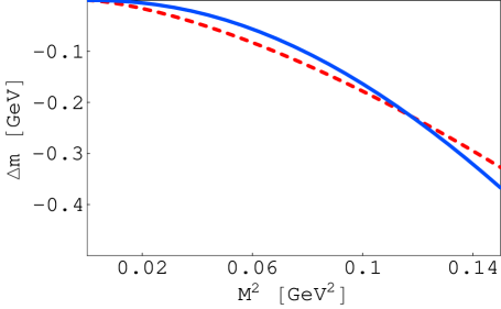
Figure 2: Pion mass dependence of the term $k_{5}M^{5}\ln(M/m_{N})$ (solid line) for $M<400$ MeV. For comparison also the term $k_{2}M^{3}$ (dashed line) is shown.

The numerical contributions from higher-order terms cannot be calculated so far since, starting with $k_{4}$, most expressions in Eq. (2) contain unknown low-energy coupling constants (LECs) from the Lagrangians of order ${\cal O}(q^{4})$ and higher. The coefficient $k_{5}$ is free of higher-order LECs and is given in terms of the axial-vector coupling constant $\texttt{g}_{A}$ and the pion-decay constant $F$. While the values for both $\texttt{g}_{A}$ and $F$ should be taken in the chiral limit, we evaluate $k_{5}$ using the physical values $g_{A}=1.2695(29)$ and $F_{\pi}=92.42(26)$ MeV. Setting $\mu=m_{N}$, $m_{N}=(m_{p}+m_{n})/2=938.92$ MeV, and $M=M_{\pi^{+}}=139.57$ MeV we obtain $k_{5}M^{5}\ln(M/m_{N})=-4.8$ MeV. This amounts to approximately $31$% of the leading nonanalytic contribution at one-loop order, $k_{2}M^{3}$. Figure 2 shows the pion mass dependence of the term $k_{5}M^{5}\ln(M/m_{N})$ (solid line) in comparison with the term $k_{2}M^{3}$ (dashed line) for $M<400$ MeV. For $M\approx 360\,\mbox{MeV}$ the $k_{5}$ term is as large as the $k_{2}$ term.

3.2 Electromagnetic Form Factors

Imposing the relevant symmetries such as translational invariance, Lorentz covariance, the discrete symmetries, and current conservation, the nucleon matrix element of the electromagnetic current operator $J^{\mu}(x)$ can be parameterized in terms of two form factors,

$$\langle N(p^{\prime})|J^{\mu}(0)|N(p)\rangle=\bar{u}(p^{\prime})\left[F_{1}^{N}(Q^{2})\gamma^{\mu}+i\frac{\sigma^{\mu\nu}q_{\nu}}{2m_{p}}F_{2}^{N}(Q^{2})\right]u(p),\quad N=p,n,$$ (3)

where $q=p^{\prime}-p$, $Q^{2}=-q^{2}$, and $m_{p}$ is the proton mass. At $Q^{2}=0$, the so-called Dirac and Pauli form factors $F_{1}$ and $F_{2}$ reduce to the charge and anomalous magnetic moment in units of the elementary charge and the nuclear magneton $e/(2m_{p})$, respectively,

$$F_{1}^{p}(0)=1,\quad F_{1}^{n}(0)=0,\quad F_{2}^{p}(0)=1.793,\quad F_{2}^{n}(0)=-1.913.$$

The Sachs form factors $G_{E}$ and $G_{M}$ are linear combinations of $F_{1}$ and $F_{2}$,

$$G_{E}^{N}(Q^{2})=F_{1}^{N}(Q^{2})-\frac{Q^{2}}{4m_{p}^{2}}F_{2}^{N}(Q^{2}),\quad G_{M}^{N}(Q^{2})=F_{1}^{N}(Q^{2})+F_{2}^{N}(Q^{2}),\quad N=p,n,$$

and, in the non-relativistic limit, their Fourier transforms are commonly interpreted as the distribution of charge and magnetization inside the nucleon. The description of the electromagnetic form factors of the nucleon presents a stringent test for any theory or model of the strong interactions.

Calculations in Lorentz-invariant baryon ChPT up to fourth order fail to describe the proton and nucleon form factors for momentum transfers beyond $Q^{2}\sim 0.1\,\mbox{GeV}^{2}$ [19, 20]. In Ref. [19] it was shown that the inclusion of vector mesons can result in the re-summation of important higher-order contributions. In Ref. [21] the electromagnetic form factors of the nucleon up to fourth order have been calculated in manifestly Lorentz-invariant ChPT with vector mesons as explicit degrees of freedom. A systematic power counting for the renormalized diagrams has been implemented using both the extended on-mass-shell renormalization scheme and the reformulated version of infrared regularization. The inclusion of vector mesons results in a considerably improved description of the form factors (see Fig. 3). The most dominant contributions come from tree-level diagrams, while loop corrections with internal vector meson lines are small [21].

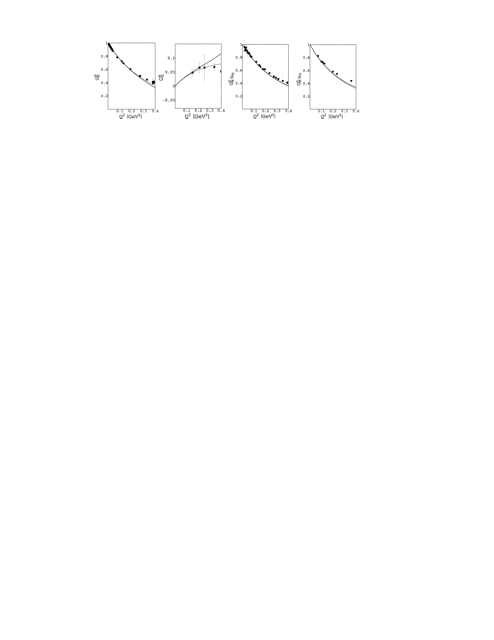
Figure 3: The Sachs form factors of the nucleon in manifestly Lorentz-invariant chiral perturbation theory at ${\cal O}(q^{4})$ including vector mesons as explicit degrees of freedom. Full lines: results in the extended on-mass-shell scheme; dashed lines: results in infrared regularization. The experimental data are taken from Ref. [22].

3.3 Axial and Induced Pseudoscalar Form Factors

Assuming isospin symmetry, the most general parametrization of the isovector axial-vector current evaluated between one-nucleon states is given by

$$\langle N(p^{\prime})|A^{\mu,a}(0)|N(p)\rangle=\bar{u}(p^{\prime})\left[\gamma^{\mu}\gamma_{5}G_{A}(Q^{2})+\frac{q^{\mu}}{2m_{N}}\gamma_{5}G_{P}(Q^{2})\right]\frac{\tau^{a}}{2}u(p),$$ (4)

where $q=p^{\prime}-p$, $Q^{2}=-q^{2}$, and $m_{N}$ denotes the nucleon mass. $G_{A}(Q^{2})$ is called the axial form factor and $G_{P}(Q^{2})$ is the induced pseudoscalar form factor. The value of the axial form factor at zero momentum transfer is defined as the axial-vector coupling constant, $g_{A}=G_{A}(Q^{2}=0)=1.2695(29)$, and is quite precisely determined from neutron beta decay. The $Q^{2}$ dependence of the axial form factor can be obtained either through neutrino scattering or pion electroproduction. The second method makes use of the so-called Adler-Gilman relation [23] which provides a chiral Ward identity establishing a connection between charged pion electroproduction at threshold and the isovector axial-vector current evaluated between single-nucleon states (see, e.g., Ref. [24, 25] for more details). The induced pseudoscalar form factor $G_{P}(Q^{2})$ has been investigated in ordinary and radiative muon capture as well as pion electroproduction (see Ref. [26] for a review).

In Ref. [27] the form factors $G_{A}$ and $G_{P}$ have been calculated in manifestly Lorentz-invariant baryon ChPT up to and including order ${\cal O}(q^{4})$. In addition to the standard treatment including the nucleon and pions, the axial-vector meson $a_{1}(1260)$ has also been considered as an explicit degree of freedom. The inclusion of the axial-vector meson effectively results in one additional low-energy coupling constant which has been determined by a fit to the data for $G_{A}(Q^{2})$. The inclusion of the axial-vector meson results in an improved description of the experimental data for $G_{A}$ (see Fig. 4), while the contribution to $G_{P}$ is small.

Figure 4: Left panel: Axial form factor $G_{A}$ in manifestly Lorentz-invariant ChPT at ${\cal O}(q^{4})$ including the axial-vector meson $a_{1}(1260)$ explicitly. Full line: result in infrared renormalization, dashed line: dipole parametrization. The experimental data are taken from Ref. [24]. Right panel: The induced pseudoscalar form factor $G_{P}$ in manifestly Lorentz-invariant ChPT at ${\cal O}(q^{4})$ including the axial-vector meson $a_{1}(1260)$ explicitly. Full line: result with axial-vector meson; dashed line: result without axial-vector meson. One can clearly see the dominant pion pole contribution at $Q^{2}\approx-M_{\pi}^{2}$.

3.4 Pion-Nucleon Form Factor

The pion-nucleon form factor $G_{\pi N}(Q^{2})$ may be defined in terms of the pseudoscalar quark density $P^{a}=i\bar{q}\gamma_{5}\tau^{a}q$ and the average light-quark mass $\hat{m}$ as [7]

$$\hat{m}\langle N(p^{\prime})|P^{a}(0)|N(p)\rangle=\frac{M_{\pi}^{2}F_{\pi}}{M_{\pi}^{2}+Q^{2}}G_{\pi N}(Q^{2})i\bar{u}(p^{\prime})\gamma_{5}\tau^{a}u(p),$$ (5)

where $q=p^{\prime}-p$, $Q^{2}=-q^{2}$, and $\Phi^{a}(x)\equiv\frac{\hat{m}P^{a}(x)}{M_{\pi}^{2}F_{\pi}}$ is the corresponding interpolating pion field. The pion-nucleon coupling constant is given by $g_{\pi N}=G_{\pi N}(-M_{\pi}^{2})$. Using the (QCD-) partially conserved axial-vector current (PCAC) relation, $\partial_{\mu}A^{\mu,a}=\hat{m}P^{a}$, the pion-nucleon form factor is completely given in terms of the axial and the induced pseudoscalar form factors,

$$2m_{N}G_{A}(Q^{2})-\frac{Q^{2}}{2m_{N}}G_{P}(Q^{2})=2\frac{M_{\pi}^{2}F_{\pi}}{M_{\pi}^{2}+Q^{2}}G_{\pi N}(Q^{2}).$$

This is an exact relation which holds true for any value of $Q^{2}$. The result at ${\cal O}(q^{4})$ is given by [27]

$$G_{\pi N}(Q^{2})=\frac{m_{N}g_{A}}{F_{\pi}}-g_{\pi N}\Delta\frac{Q^{2}}{M_{\pi}^{2}}+\cdots$$

where $\Delta=1-\frac{m_{N}g_{A}}{F_{\pi}g_{\pi N}}$ denotes the Goldberger-Treiman discrepancy. The chiral expansion of the pion-nucleon coupling constant can be found in Ref. [27].

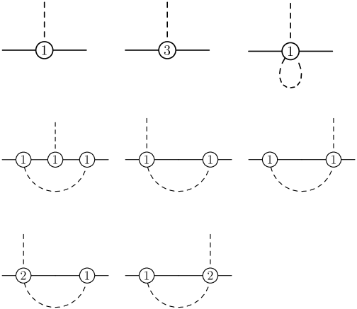
Figure 5: Diagrams contributing to the pion-nucleon vertex at ${\cal O}(q^{4})$.

Finally, we would like to stress that one carefully has to distinguish between the pion-nucleon form factor $G_{\pi N}(Q^{2})$ of Eq. (5) on the one hand and the renormalized pion-nucleon vertex in ChPT on the other hand. The unrenormalized vertex, when evaluated between on-shell nucleon states, is of the form

$$\Gamma_{5}(q^{2})\gamma_{5}\tau^{a}.$$ (6)

At ${\cal O}(q^{4})$ one needs to calculate the diagrams shown in Fig. 5. In general, the pion-nucleon vertex depends on the choice of the field variables in the effective Lagrangian. Only at $q^{2}=M_{\pi}^{2}$, we expect the same coupling strength, since both $\hat{m}P^{a}(x)/(M_{\pi}^{2}F_{\pi})$ and the field $\pi^{a}$ of Eq. (1) serve as interpolating pion fields:

$$G_{\pi N}(-M_{\pi}^{2})=g_{\pi N}=Z_{\Psi}\sqrt{Z_{\pi}}\Gamma_{5}(M_{\pi}^{2}).$$

On the other hand, for arbitrary $q^{2}$

$$G_{\pi N}(Q^{2})\neq Z_{\Psi}\sqrt{Z_{\pi}}\Gamma_{5}(q^{2}).$$

In the present case, the pion-nucleon vertex is only an auxiliary quantity, whereas the “fundamental” quantity (entering chiral Ward identities) is the matrix element of the pseudoscalar density.

4 Summary and Conclusion

Both the infrared regularization and the EOMS scheme allow for a simple and consistent power counting in manifestly Lorentz-invariant baryon chiral perturbation theory. We have discussed some results of a two-loop calculation of the nucleon mass. The inclusion of vector and axial-vector mesons as explicit degrees of freedom leads to an improved phenomenological description of the electromagnetic and axial form factors, respectively. Work on the application to electromagnetic processes such as Compton scattering and pion production is in progress.

I would like to thank D. Djukanovic, T. Fuchs, J. Gegelia, G. Japaridze, and M. R. Schindler for the fruitful collaboration on the topics of this talk. This work was made possible by the financial support from the Deutsche Forschungsgemeinschaft (SFB 443 and SCHE 459/2-1) and the EU Integrated Infrastructure Initiative Hadron Physics Project (contract number RII3-CT-2004-506078).

References

- [1] S. Weinberg, Physica A 96 (1979) 327
- [2] J. Gasser and H. Leutwyler, Annals Phys. 158 (1984) 142
- [3] S. Scherer, Adv. Nucl. Phys. 27 (2003) 277
- [4] S. Scherer and M. R. Schindler, arXiv:hep-ph/0505265
- [5] J. Bijnens, Prog. Part. Nucl. Phys. 58 (2007) 521
- [6] V. Bernard, arXiv:0706.0312 [hep-ph]
- [7] J. Gasser, M. E. Sainio, and A. Švarc, Nucl. Phys. B 307 (1988) 779
- [8] S. Weinberg, The Quantum Theory of Fields. Vol. 1: Foundations (Cambridge University Press, Cambridge, UK, 1995)
- [9] J. Gegelia, G. S. Japaridze, and K. S. Turashvili, Theor. Math. Phys. 101 (1994) 1313
- [10] T. Becher and H. Leutwyler, Eur. Phys. J. C 9 (1999) 643
- [11] T. Fuchs, J. Gegelia, G. Japaridze, and S. Scherer, Phys. Rev. D 68 (2003) 056005
- [12] T. Fuchs, M. R. Schindler, J. Gegelia, and S. Scherer, Phys. Lett. B 575 (2003) 11
- [13] C. Hacker, N. Wies, J. Gegelia, and S. Scherer, Phys. Rev. C 72 (2005) 055203
- [14] M. R. Schindler, J. Gegelia, and S. Scherer, Phys. Lett. B 586 (2004) 258
- [15] M. R. Schindler, J. Gegelia, and S. Scherer, Nucl. Phys. B 682 (2004) 367
- [16] M. R. Schindler, D. Djukanovic, J. Gegelia, and S. Scherer, Phys. Lett. B 649 (2007) 390
- [17] M. R. Schindler, D. Djukanovic, J. Gegelia, and S. Scherer, arXiv:0707.4296 [hep-ph]
- [18] J. A. McGovern and M. C. Birse, Phys. Lett. B 446 (1999) 300
- [19] B. Kubis and U.-G. Meissner, Nucl. Phys. A 679 (2001) 698
- [20] T. Fuchs, J. Gegelia, and S. Scherer, J. Phys. G 30 (2004) 1407
- [21] M. R. Schindler, J. Gegelia, and S. Scherer, Eur. Phys. J. A 26 (2005) 1
- [22] J. Friedrich and Th. Walcher, Eur. Phys. J. A 17 (2003) 607
- [23] S. L. Adler and F. J. Gilman, Phys. Rev. 152 (1966) 1460
- [24] V. Bernard, L. Elouadrhiri, and U. G. Meissner, J. Phys. G 28 (2002) R1
- [25] T. Fuchs and S. Scherer, Phys. Rev. C 68 (2003) 055501
- [26] T. Gorringe and H. W. Fearing, Rev. Mod. Phys. 76 (2004) 31
- [27] M. R. Schindler, T. Fuchs, J. Gegelia, and S. Scherer, Phys. Rev. C 75 (2007) 025202