Throughput Optimal On-Line Algorithms for Advanced Resource Reservation in Ultra High-Speed Networks

Abstract

Advanced channel reservation is emerging as an important feature of ultra high-speed networks requiring the transfer of large files. Applications include scientific data transfers and database backup. In this paper, we present two new, on-line algorithms for advanced reservation, called $\mathtt{BatchAll}$ and $\mathtt{BatchLim}$, that are guaranteed to achieve optimal throughput performance, based on multi-commodity flow arguments. Both algorithms are shown to have polynomial-time complexity and provable bounds on the maximum delay for $1+\varepsilon$ bandwidth augmented networks. The $\mathtt{BatchLim}$ algorithm returns the completion time of a connection immediately as a request is placed, but at the expense of a slightly looser competitive ratio than that of $\mathtt{BatchAll}$. We also present a simple approach that limits the number of parallel paths used by the algorithms while provably bounding the maximum reduction factor in the transmission throughput. We show that, although the number of different paths can be exponentially large, the actual number of paths needed to approximate the flow is quite small and proportional to the number of edges in the network. Simulations for a number of topologies show that, in practice, 3 to 5 parallel paths are sufficient to achieve close to optimal performance. The performance of the competitive algorithms are also compared to a greedy benchmark, both through analysis and simulation.

I Introduction

TCP/IP has been so far considered and used as the core infrastructure for all sorts of data transfer including bulk FTP applications. Yet, it has recently been observed that in ultra high speed networks, there exists a large gap between the capacity of network links and the maximum end-to-end throughput achieved by TCP [1, 2]. This gap, which is mainly attributed to the shared nature of Internet traffic, is becoming increasingly problematic for modern Grid and data backup applications requiring transfer of extremely large datasets on the orders of terabytes and more.

These limitations have raised efforts for development of an alternative protocol stack to complement TCP/IP. This protocol stack is based on the concept of advanced reservation [2, 3], and is specifically tailored for large file transfers and other high throughput applications. The most important property of advanced reservation is to offer hosts and users the ability to reserve in advance dedicated paths to connect their resources. The importance of advanced reservation in supporting dedicated connections has been made evident by the growing number of testbeds related to this technology, such as UltraScience Net [2], On-demand Secure Circuits and Advanced Reservation Systems (OSCARS) [4], and Dynamic Resource Allocation via GMPLS Optical Networks (DRAGON) [5].

Several protocols and algorithms have been proposed in the literature to support advance reservation, see, e.g., [2, 6, 3] and references therein. To the authors’ knowledge, none of them guarantees the same throughput performance as an optimal off-line algorithm. Instead, most are based on greedy approaches, whereas each request is allocated a path guaranteeing the earliest completion time at the time the request is placed.

Our first contribution in this paper is to uncover fundamental limitations of greedy algorithms. Specifically, we show that there exist network topologies and request patterns for which the maximum throughput of these algorithms can be arbitrarily smaller than the optimal throughput, as the network size grows.

Next, we present competitive advanced reservation algorithms that provably achieve the maximum throughput for any network and request profile. The first algorithm, called $\mathtt{BatchAll}$, provides a competitive ratio on the maximum delay experienced by each request in an augmented resource network with respect to the optimal off-line algorithm in the original network. $\mathtt{BatchAll}$ groups requests into batches. In each batch, paths are efficiently assigned based on a maximum concurrent flow optimization. All the requests arriving during a current batch must wait until its completion before being assigned to the next batch.

The $\mathtt{BatchAll}$ algorithm does not return the connection completion time to the user at the time a request is placed, but only when the connection actually starts. Our second algorithm, called $\mathtt{BatchLim}$, returns the completion time immediately as a request is placed, but at the expense of a slightly looser competitive ratio. This algorithm operates by limiting the length of each batch.

The presented competitive algorithms are based upon multicommodity flow algorithms, and therefore can be performed efficiently in polynomial time in the size of the network for each request.

Our model assumes that the network infrastructure supports path dispersion, i.e., multiple paths in parallel can be used to route data. Obviously, a too large path dispersion may be undesirable, as it may entail fragmenting a file into a large number of segments and reassembling them at the destination. To address this issue, we present a simple approach, based on the max-flow min-cut theorem, that limits the number of parallel paths while bounding the maximum reduction factor in the transmission throughput. We prove that this bound is tight. We, then, propose two algorithms $\mathtt{BatchAllDisp}$ and $\mathtt{BatchLimDisp}$, based upon $\mathtt{BatchAll}$ and $\mathtt{BatchLim}$ respectively. These algorithms perform similarly to the original algorithms, in terms of the batching process. However, after filling each batch, the algorithms will limit the dispersion of each flow. Although these algorithms are not throughput optimal anymore, they are still throughput competitive.

While the main emphasis of this paper is on the derivation of theoretical performance guarantees on the maximum throughput of advanced reservation protocols, we also provide simulation results illustrating the performance of these protocols in terms of the average delay. The simulations show that the proposed competitive algorithms compare favorably to a greedy benchmark, although the benchmark does sometime exhibit superior performance, especially in sparse topologies or at low load. With respect to path dispersion, we show that excellent performance can be achieved with as few as five or so parallel paths per connection.

Note that preliminary findings leading to this work were reported in a two-page abstract [7]. The only overlap is Lemma IV.1 and Theorem IV.3, which were presented without proof.

This paper is organized as follows. In Section II, we briefly scan the related work on advanced reservation, competitive approaches, and path dispersion. In Section III, we introduce our model and notation used throughout the paper. We also present natural greedy approaches and demonstrate their inefficiency. In Section IV, we describe the $\mathtt{BatchAll}$ and $\mathtt{BatchLim}$ algorithms and derive results on their competitive ratios. Our method for bounding path dispersion is described and analyzed in Section V. In Section VI, simulation results evaluating the performance of some of our algorithms under different network topologies and traffic parameters are presented. We conclude the paper in Section VII.

II Related Work

Competitive algorithms for advanced reservation networks is the focus of [8]. This work discusses the lazy ftp problem, where reservations are made for channels for the transfer of different files. The algorithm presented there provides a 4-competitive algorithm for the makespan (the total completion time). However, [8] focuses on the case of fixed routes. When routing is also to be considered, the time complexity of the algorithm presented there may be exponential in the network size.

Another recent work [9], focusing on routing in packet switched network in an adversarial setting, discusses choosing routes for fixed size packets injected by an adversary. It enforces regularity limitations on the adversary which are stronger than the ones required here, and achieves the network capacity with a guarantee on the maximum queue size. It does not discuss the case of advance reservation with different job sizes or bandwidth requirements. It is based upon approximating an integer programming, which may not be extensible to a case where path reservation, rather than packet-based routing is involved.

Most of the works regarding competitive approaches to routing focused mainly on call admission, without the ability of advance reservation. For some results in this field see, e.g., [10, 11]. Some results involving advanced reservation are presented in [12]. However, the path selection there is based on several alternatives supplied by a user in the request rather than a path selection using an automated mechanism attempting to optimize performance, as discussed here. In [13] a combination of call admission and circuit switching is used to obtain a routing scheme with a logarithmic competitive ratio on the total revenue received. A competitive routing scheme in terms of the number of failed routes in the setting of ad-hoc networks is presented in [14]. A survey of on-line routing results is presented in [15]. A competitive algorithm for admission and routing in a multicasting setting is presented in [16]. Most of the other existing work in this area consists of heuristic approaches which main emphasis are on the algorithm correctness and computational complexity, without throughput guarantees.

In [17] a rate achieving scheme for packet switching at the switch level is presented. Their scheme is based on convergence to the optimal multicommodity flow using delayed decision for queued packets. Their results somewhat resemble our $\mathtt{BatchAll}$ algorithm. However, their scheme depends on the existence of an average packet size, whereas our scheme addresses the full routing-scheduling question for any size distribution and any (adversarial) arrival schedule. In [18] queuing analysis of several optical transport network architectures is conducted, and it is shown that under some conditions on the arrival process, some of the schemes can achieve the maximum network rate. As the previous one, this paper does not discuss the full routing-scheduling question discussed here and does not handle unbounded job sizes. Another difference is that our paper provides an algorithm, $\mathtt{BatchLim}$ discussed below, guaranteeing the ending time of a job at the time of arrival, which, as far as we know is the first such algorithm.

Many papers have discussed the issue of path dispersion and attempted to achieve good throughput with limited dispersion, a survey of some results in this field is given in [19]. In [20, 21] heuristic methods of controlling multipath routing and some quantitative measures are presented. As far as we know, our work proposes the first formal treatment allowing the approximation of a flow using a limited number of paths with any desired accuracy.

III Greedy Algorithms and their Limitations

III-A Network Model

We first present the network model that will be used throughout the paper (both for the greedy and competitive algorithms). The model consists of a general network topology, represented by a graph $G(V,E)$, where $V$ is the set of nodes and $E$ is the set of links connecting the nodes. The graph $G$ can be directed or undirected. The capacity of each link $e\in E$ is $C(e)$. A connection request, also referred to as job, contains the tuple $(s,d,f)$, where $s\in V$ is the source node, $d\in V-\{s\}$ is the destination node, and $f$ is the file size.

Accordingly, an advance reservation algorithm computes a starting time at which the connection can be initiated, a set of paths used for the connection, and an amount of bandwidth allocated to each path. Our model supports path dispersion, i.e., multiple paths in parallel can be used to route data (in section V-B, we discuss practical methods to bound path dispersion while still providing performance guarantees). In addition, the greedy algorithms introduced below employ path switching, whereby a connection is allowed to switch between different paths throughout its duration.

In subsequent sections, we will make frequent use of multicommodity functions. The multicommodity flow problem is a linear planning problem returning $\mathtt{true}$ or $\mathtt{false}$ based upon the feasibility of transmitting concurrent flows from all pairs of sources and destination during a given time duration, such that the total flow through each link does not exceed its capacity. It is solved by a function $\mathtt{multicomm}(G,L,T)$, where $L$ is a list of jobs, each containing a source, a destination, and a file size, and $T$ is the time duration.

In the sequel of this paper, we will be interested in characterizing the saturation throughput of the various algorithms, which is defined as the maximum arrival rate of requests such that the average delay experienced by requests is still finite (delay is defined as the time elapsing between the arrival of a connection request until the completion of the corresponding connection).

The maximum concurrent flow is calculated by the function $\mathtt{maxflow}(G,L)$. It returns $T_{\mathrm{min}}$, the minimum value of $T$ such that $\mathtt{multicomm}(G,L,T)$ returns $\mathtt{true}$. Both the multicommodity and maximum concurrent flow problems are known to be computable in polynomial time [22, 23].

III-B Algorithms

$\mathtt{Greedy}$

A seemingly natural way to implement advanced channel reservation is to follow a greedy procedure, where, at the time a request is placed, the request is allocated a path (or set of paths) guaranteeing the earliest possible completion time. We refer to this approach as $\mathtt{Greedy}$ and explain it next.

The $\mathtt{Greedy}$ algorithm divides the time axis into slots delineated by event. Each event corresponds to a set up or tear down instance of a connection. Therefore, during each time slot the state of all links in the network remains unchanged. In general, the time axis will consist of $n$ time slots, where $n\geq 1$ is a variable and slot $i$ corresponds to time interval $[t_{i},t_{i+1}]$. Note that $t_{1}=t$ (the time at which the current request is placed) and $t_{n+1}=\infty$.

Let $W_{i}={\{b_{i}(1),b_{i}(2),\ldots,b_{i}(|E|)}\}$ be the vector of reserved bandwidth on all links at time slot $i$ where $i=1,\ldots,n$, and $b_{i}(e)$ denote the reserved bandwidth on link $e$ during slot $i$, with $e=1,\ldots,|E|$.

For each slot $i\in L$, construct a graph $G_{i}$, where the capacity of link $e\in E$ is $C_{i}(e)=C(e)-b_{i}(e)$, i.e., $C_{i}(e)$ represents the available bandwidth on link $e$ during slot $i$.

In order to guarantee the earliest completion time, $\mathtt{Greedy}$ repeatedly performs a max flow allocation between nodes $s$ and $d$, for as many time slots as needed until the entire file is transferred. This approach ensures that, in each time slot, the maximum possible number of bits is transmitted and, hence, the earliest possible completion time (at the time the request is placed) is achieved. The $\mathtt{Greedy}$ algorithm can thus be concisely described with the following pseudo-code:

1. Initialization

   • Set initial time slot: $i$=1.

   • Set initial size of remaining file: $r=f$.

2. If $\mathtt{maxflow}(G_{i},s,d,r)\geq t_{i+1}-t_{i}$ (i.e., all the remaining file can be transferred during the current time slot) then

3. Exit step:

   • Update $W_{i}$ by subtracting the used bandwidth from every link in the new flow and, if needed, create a new event $t_{i+1}$ corresponding to end of connection.

   • Exit procedure.

   else

4. Non-exit step:

   • Update $W_{i}$ by subtracting the used bandwidth from every link in the new flow.

   • $r=r-r\times(t_{i+1}-t_{i})/\mathtt{maxflow}(G_{i},s,d,r)$ (update size of remaining file).

   • $i=i+1$ (advance to the next time slot).

   • Go back to step 2.

$\mathtt{Greedy\_shortest}$

The $\mathtt{Greedy\_shortest}$ algorithm is a variation of $\mathtt{Greedy}$, where only shortest paths (in terms of number of hops) between the source $s$ and destination $d$ are utilized to route data. To implement $\mathtt{Greedy\_shortest}$, we employ exactly the same procedure as in $\mathtt{Greedy}$, except that we prune all the links not belonging to one of the shortest paths using breadth first search. Note that for a given source $s$ and destination $d$, the pruned links are the same for all the graphs $G_{i}$.

III-C Inefficiency Results

We next constructively show that there exist certain arrival patterns, for which both $\mathtt{Greedy}$ and $\mathtt{Greedy\_shortest}$ achieve a saturation throughput significantly lower than optimal. Specifically, we present cases where the saturation throughput of $\mathtt{Greedy}$ and $\mathtt{Greedy\_shortest}$ is $\Omega(|V|)$ times smaller than the optimal throughput. Thus, the ratio of the maximum throughput of the greedy algorithms to that of the optimal algorithm can be arbitrarily small.

Theorem III.1

For any given vertex set with cardinality $|V|$, there exists a graph $G(V,E)$ such that the saturation throughput of $\mathtt{Greedy}$ is $|V|/2$ times smaller than the optimal saturation throughput.

Proof:

Consider the ring network shown in Fig. 1(a). Suppose every link is an undirected 1 Gb/s link and that during each second requests arrive in this order: 1Gb request from node 1 to 2, 1Gb request from node 2 to 3, 1Gb request from node 3 to 4, $\cdots$, 1Gb request from node $|V|$ to 1.

The $\mathtt{Greedy}$ algorithm will allocate the maximum flow to each request, meaning it will be split to two paths, half flowing directly, and half flowing through the alternate path along the entire ring. Therefore, each new request will have to wait to the previous one to end, resulting in a completion time of $|V|/2$ seconds.

On the other hand, the optimal time is just one second using the direct link between each pair of nodes. Assuming the above pattern of requests repeats periodically, then an optimal algorithm can support at most one request per second between each pair of neighboring nodes before reaching saturation, while $\mathtt{Greedy}$ can support at most $2/|V|$ request per second, hence proving the theorem. A similar result can be proved for directed graphs.        $\square$

We next show that restricting routing to shortest paths does not solve the inefficiency problem.

Theorem III.2

For any given vertex set cardinality $|V|$, there exists a graph $G(V,E)$ such that the saturation throughput of $\mathtt{Greedy\_shortest}$ (or any other algorithm using only shortest path routing) is $|V|-2$ times smaller than the optimal saturation throughput.

Proof:

Consider the network depicted in Fig. 1(b), where all requests are from node 1 to 2, and only the direct path is used by the algorithm. In this scenario, an optimal algorithm would all $|V|-2$ paths between nodes 1 and 2. Hence, the optimal algorithm can achieve a saturation throughput $|V|-2$ higher than $\mathtt{Greedy\_shortest}$.        $\square$

Figure 1: Examples for the disadvantages of the greedy approach.

IV Competitive Algorithms

In the previous section, we uncovered some of the limitations of greedy algorithms that immediately allocate resources to each arriving request. In this section, we present a new family of on-line, polynomial-time algorithms that rely on the idea of “batching” requests. Thus, instead of immediately reserving a path for each incoming request as in the greedy algorithms, we accumulate several arrivals in a batch and assign a more efficient set of flow paths to the whole batch. The proposed algorithms guarantee that the maximum delay experienced by each request is within a finite multiplicative factor of the value achieved with an optimal off-line algorithm. Thus, these algorithms reach the maximum throughput achievable by any algorithm.

IV-A Capacity Bounds

As a preparatory step, we present a bound on the maximum throughput achievable by any algorithm. This bound, based on a multicommodity flow formulation, will be used to compare the performance of the proposed on-line competitive algorithms to the optimal off-line algorithm.

Lemma IV.1

If during any time interval $T$, each node $i\in V$ sends on average $\gamma_{ij}$ bits of information per unit time to node $j\in V-\{i\}$, then there exists a multi-commodity flow allocation on graph $G$ with flow values $f_{ij}=\gamma_{ij}$.

Proof:

First, we prove that for any given arrangement of sources and destinations in a network and at any time $t$, the transmission rates in bits per unit time comply with the properties of multi-commodity flows. Take the transmission rate between node $i$ and $j$ going through the (directed) edge $k$ at time $t$ to be $R^{k}_{i,j}(t)$. The total throughput passing each link can not exceed the link capacity, $\sum_{i,j}R^{k}_{i,j}(t)\leq C(k)$. According to the information conservation property, the total transmission rate into any node is equal to the out-going rate except for the source and destination of any of the transmissions. Now, the average transmissions during any time interval $T$ satisfy the same properties as above because of linearity. Thus, we obtain a valid multi-commodity flow problem, where the time average of each flow represents an admissible commodity.        $\square$

Corollary IV.2

The average transmission rate between all pairs in the network for any time interval is a feasible multicommodity flow.

IV-B The $\mathtt{BatchAll}$ Competitive Algorithm

In case no deterministic knowledge on the future requests is given, one would like to give some bounds on the performance of the algorithm compared to the performance of a “perfect” off-line algorithm (i.e., with full knowledge of the future and unlimited computational resources). We present here an algorithm, called $\mathtt{BatchAll}$ (since it batches together all pending requests), giving bounds on this measure.

The algorithm can be described as follows (we assume that there is initially no pending request):

1. For a request $l=\{s,d,f\}$ arriving at time $t$, give an immediate starting time and an ending time of $t_{c}=t+\mathtt{maxflow}(G,l)$.

2. Set $L\leftarrow\mbox{null}$.

3. While $t<t_{c}$ and another request $l^{\prime}=\{s^{\prime},d^{\prime},f^{\prime}\}$ arrives at time $t$:

   • Set $L\leftarrow L\cup l^{\prime}.$

   • Mark $t_{c}$ as its starting time and add it to the waiting batch.

4. When $t=t_{c}$, calculate $t^{\prime}=\mathtt{maxflow}(G,L)$.

   • If $t^{\prime}=0$ (i.e., there is no pending request) go back to step 1.

   • Else $t_{c}=t_{c}+t^{\prime}$ and go back to step 2.

We note that upon the arrival of a request, the $\mathtt{BatchAll}$ algorithm returns only the starting time of the connection. The allocated paths and completion time are computed only when the connection starts (in the next section, we present another competitive algorithm with a slightly looser competitive ratio but which returns the completion time at the arrival time of a request).

We next compare the performance of an optimal off-line algorithm in the network with that of the $\mathtt{BatchAll}$ algorithm in an augmented network. The augmented network is similar to the original network, other than that it has a capacity of $(1+\varepsilon)C(e)$ at any link, $e$, that has capacity $C(e)$ in the original network. This implies that the performance of the competitive algorithm is comparable if one allows a factor $\varepsilon$ extra capacity in the links, or, alternatively, one may say that the performance of the algorithm is comparable to the optimal off-line algorithm in some lower capacity network, allowing the maximum rate of only $(1+\varepsilon)^{-1}C(e)$ for each link. The $\mathtt{BatchAll}$ algorithm satisfies the following theoretical property on the maximum waiting time:

Theorem IV.3

In a network with augmented resources where every edge has bandwidth $(1+\varepsilon)$ times the original bandwidth (for all $\varepsilon>0$), the maximum waiting time from request arrival to the end of the transmission using $\mathtt{BatchAll}$, for requests arriving up to any time $t^{*}$, is no more than $2/\varepsilon$ times the maximum waiting time for the optimal algorithm in the original network.

Proof:

Consider the augmented resource network. Take the maximum length batch that accommodates requests arriving before time $t^{*}$, say $i$, and mark its length by $T$. Since the batch before this one was of length at most $T$ (if a request arrives when no batch is executing, the batch is considered to be of size 0), and all requests in batch $i$ were received during the execution of previous batch $i-1$, then the total waiting time of each of these requests was at most $2T$. By Corollary IV.2, the total time for handling all requests received during the execution of batch $i-1$ must have been at least $T$ in the augmented network, or $(1+\varepsilon)T$ in the original network. Since all of these requests arrived during a time of at most $T$, one of them must have been continuing at least a time of $\varepsilon T$ after the last request under any algorithm. Therefore the ratio between the maximum waiting time is at most $2/\varepsilon$.        $\square$

Corollary IV.4

The saturation throughput of $\mathtt{BatchAll}$ is optimal because for any arbitrarily small $\epsilon>0$, the delay of a request is guaranteed to be at most a finite multiplicative factor larger than the maximum delay of the optimal algorithm in the reduced resources network.

We next show that the computational complexity of $\mathtt{BatchAll}$ is practical.

Theorem IV.5

The computational complexity of algorithm $\mathtt{BatchAll}$ per request is at most polynomial in the size of the network.

Proof:

For each batch, the $\mathtt{BatchAll}$ algorithm solves a maximum concurrent flow problem that can be computed in polynomial time [22]. Noting that the number of batches cannot exceed the number of requests (since each batch contains at least one request), the theorem is proven.        $\square$

IV-C The $\mathtt{BatchLim}$ Competitive Algorithm

The following algorithm, called $\mathtt{BatchLim}$, operates in a similar setup to $\mathtt{BatchAll}$. However, it gives a guarantee on the finishing time of a job when it is submitted.

The algorithm is based on creating increasing size batches in case of high loads. When the rate of request arrival is high, each batch created will be approximately twice as long as the previous one, and thus larger batches, giving a good approximation of the total flow will be created. When the load is low only a single batch of pending requests exists at most times, and its size will remain approximately constant or even decrease for decreasing load.

The algorithm maintains a list of times, $t_{i}$, $i=1,\ldots,n$, where for every interval, $[t_{i},t_{i+1}]$, a batch of jobs is assigned. When a new request between a source $s$ and a destination $d$ arrives at time $t$, then an attempt is first made to add it to one of the existing intervals by using a multicommodity flow calculation. If the attempt fails, a new time, then a new batch is created and $t_{n+1}=\max(t_{n}+(t_{n}-t),t_{n}+M)$, where $M=f/\mathtt{maxflow}(G,s,d)$ is the minimum time for the job completion, is added to the list, and the job is assigned to the interval $[t_{n},t_{n+1}]$.

We next provide a detailed description of how the algorithm handles a new request. We use the tuple $l=\{s,f,d\}$ to denote this job and the list $L_{i}$ to denote the set of jobs already assigned to slot $i$.

1. Initialization: set $i\leftarrow 1$.

2. While $i\leq n$

   • If $\mathtt{multicomm}(G,L_{i}\cup l,t_{i+1}-t_{i})=\mathtt{true}$ then return $i$ and exit (check if request can be accommodated during slot $i$).

   • $i\leftarrow i+1$.

3. Set $n\leftarrow n+1$ (create a new slot).

4. Set $M=\mathtt{maxflow}(G,l)$.

5. If $M>t_{n-1}-t$
   then $t_{n+1}\leftarrow t_{n}+M$;
   else $t_{n+1}\leftarrow t_{n}+(t_{n}-t)$.

6. Return $n$.

Fig. 2 illustrates runs of the $\mathtt{BatchAll}$ and $\mathtt{BatchLim}$ algorithms for the same set of requests.

The advantage of the $\mathtt{BatchLim}$ algorithm over $\mathtt{BatchAll}$ is the assignment of a completion time to a request upon its arrival. Furthermore, the proof of the algorithm requires only an attempt to assign a new job to the last interval, rather than to all of them. Therefore, it is also possible to give the details of the selected paths to the source as soon as a new batch is created.

We introduce the following technical Lemma which will be used to prove the main theorem.

Lemma IV.6

(a) For any $i$, $t_{i}-t_{i-1}\geq(t_{i}-t)/2$. (b) For any $i$, $t_{i+1}-t_{i}\leq\max(2(t_{i}-t_{i-1}),M)$, where $M$ is the minimum completion time for the largest job in the interval $[t_{i+1},t_{i}]$.

Proof:

(a) When the time slot $[t_{i-1},t_{i}]$ is added, its length is the maximum of $M$ and $[t,t_{i-1}]$. As $t$ increases $t_{i}-t_{i-1}\geq t_{i-1}-t$, and therefore $2(t_{i}-t_{i-1})\geq(t_{i}-t_{i-1})+(t_{i-1}-t)=t_{i}-t$.

(b) From (a) follows that at the time $t$ when $[t_{i+1},t_{i}]$ is added $t_{i}-t_{i-1}\geq(t_{i}-t)/2$. Since $t_{i+1}-t_{i}=\max(t_{i}-t,M)$ the Lemma follows.        $\square$

Theorem IV.7

For every $\varepsilon>0$ and every time $t^{*}$, the maximum waiting time from the request time to the end of a job for any request arriving up to time $t^{*}$ and for a network with augmented resources, is no more than $4/\varepsilon$ times the maximum waiting time for the optimal algorithm in the original network.

Proof:

When creating a new batch, at the interval $[t_{n},t_{n+1}]$ there are two possibilities:

1. $t_{n+1}=t_{n}+M$, where $M$ is the minimum time for the new job completion. In this case, the minimum time for the completion of the job in the original network would have been $(1+\varepsilon)M$. By Lemma IV.6(a) the total waiting time for the job here is at most $2M$, and therefore the ratio of waiting times is $2/(1+\varepsilon)<4/\varepsilon$.

2. $t_{n+1}=t_{n}+(t_{n}-t)$, in this case, there exists a request among the set of tasks in batch $n$ that according to theorem IV.3 waits for a time of at least $(t_{n}-t_{n-1})$. Therefore, the maximum waiting time in the original network is at least $\varepsilon(t_{n}-t_{n-1})$. Since $t_{n}-t_{n-1}\geq(t_{n}-t)/2$, and $t_{n+1}=t_{n}+t_{n}-t$, it follows that $t_{n+1}-t\leq 4(t_{n}-t_{n-1})$. Therefore, the ratio is at most $4/\varepsilon$.

$\square$

Figure 2: Illustration of the batching process by the algorithms $\mathtt{BatchAll}$ and $\mathtt{BatchLim}$. The odd numbered jobs request one hour of maximum bandwidth traffic between nodes $A$ and $B$ and the even numbered jobs request one hour maximum bandwidth traffic between $B$ and $C$. In $\mathtt{BatchAll}$, a new batch is created for all requests arriving during the running of a previous batch. In $\mathtt{BatchLim}$, for each new request an attempt is made to add it to one of the existing windows, and if it fails, a new window is appended at the end.

V Bounding Path Dispersion

V-A Approximating flows by single circuits

The algorithms presented in the previous sections (both greedy and competitive), do not limit the path dispersion, i.e., the number of number of paths simultaneously used by a connection. In practice, it is desirable to minimize the number of such paths due to the cost of setting up many paths and the need to split a into many low capacity channels. The following suggests a method of achieving this goal.

Lemma V.1

In every flow of size $F$ between two nodes on a directed graph $G(V,E)$ there exists a path of capacity at least $F/|E|$ between these nodes.

Proof:

Remove all edges of capacity (strictly) less than $F/|E|$ from the graph. The total capacity of these edges is smaller than $F/|E|\times|E|=F$. By the Max-Flow–Min-Cut theorem, the maximum flow equals the minimum cut in the network. Therefore, since the total flow is $F$ there must remain at least one path between the nodes after the removal. All edges in this path have capacity of at least $F/|E|$. Therefore, the path capacity is at least $F/|E|$.        $\square$

Lemma V.1 is tight in order in both $|E|$ and $|V|$ as can be seen for the network in Fig. 3. In this network each path amounts for only $O(|E|^{-1})=O(|V|^{-2})$ of the total flow between nodes $1$ and $2$. Therefore, to obtain a flow that consists of a given fraction of the maximum flow at least $O(|E|)=O(|V|^{2})$ of paths must be used.

Figure 3: A network demonstrating the optimality of Lemma V.1.

The following theorem establishes the maximum number of paths needed to achieve a throughput with a constant factor of that achieved by the original flow.

Theorem V.2

For every flow of size $F$ between two nodes on a directed graph $G(V,E)$ and for every $\alpha>0$ there exists a set of at most $\lceil\alpha|E|\rceil$ paths achieving a flow of at least $(1-e^{-\alpha})F$.

Proof:

Apply Lemma V.1, $\lceil\alpha|E|\rceil$ times. Each time an appropriate path is found, its flow is removed from all of its links. For each such path the remaining flow is multiplied by at most $1-\frac{1}{|E|}\leq\exp\left(\frac{1}{|E|}\right)$.        $\square$

V-B Competitive Algorithms

Theorem V.2 provides both an algorithm for reducing the number of paths and a bound on the throughput loss. To approximate the flow by a limited number of paths remove all edges with capacity less than $F/|E|$ and find a remaining path. This process can be repeated to obtain improving approximations of the flow. The maximum number of paths needed to achieve an approximation of the flow to within a constant factor is linear in $|E|$, while the number of possible paths may be exponential in $|E|$.

Using the above approximation in conjunction with the competitive algorithms one can devise two new algorithms $\mathtt{BatchAllDisp}$ and $\mathtt{BatchLimDisp}$, based upon $\mathtt{BatchAll}$ and $\mathtt{BatchLim}$ respectively. These algorithms perform similarly to $\mathtt{BatchAll}$ and $\mathtt{BatchLim}$, in terms of the batching process. However, after filling each batch, the algorithms will limit the dispersion of each flow, and approximate the flow. To achieve a partial flow, each time we select the widest path from remaining edges (where the weights are determined by the link utilization in the solution of the multicommodity flow) and reserve the total path bandwidth. We repeat this until either the desired number of paths is reached or the entire flow is routed. Setting the dispersion bound to $\alpha|E|$, Theorem V.2 guarantees that the time allocated for the slot will be no more than $\mathtt{maxflow}(G,L)/(1-e^{-\alpha})$, where $\mathtt{maxflow}(G,L)$ is the original slot duration. Algorithms $\mathtt{BatchAllDisp}$ and $\mathtt{BatchLimDisp}$ will achieve a throughput within a factor of $1-e^{-\alpha}$ of the maximum throughput (and will no longer be throughput optimal as $\mathtt{BatchAll}$ and $\mathtt{BatchLim}$, but only throughput competitive).

VI Simulations

In this section, we present simulation results illustrating the performance of the algorithms described in this paper. While the emphasis of the previous sections was on the throughput optimality (or competitiveness) of our proposed algorithms, here we are also interested in evaluating their performance for other metrics, especially average delay. Average delay is defined as the average time elapsing from the point a request is placed until the corresponding connection is completed.

The main points of interest are as follows: (1) how do the competitive algorithms fare compared to the greedy approach of Section III? (2) what value of path dispersion is needed to ensure good performance? It is important to emphasize that we do not expect the throughput optimal competitive algorithms to always outperform the greedy approach in terms of average delay.

VI-A Simulation Set-Up

We have written our own in simulator in C++. The simulator uses the COIN-OR Linear Program Solver (CLP) library [24] to solve multi-commodity optimization problems and allows evaluating our algorithms under various topological settings and traffic conditions. The main simulation parameters are as follows:

(a) 8 node

(b) 11 node LambdaRail

Figure 4: Simulation topologies.

• Topology: our simulator supports arbitrary topologies. In this paper, we consider the two topologies depicted in Figure 4. One is a fully connected graph (clique) of eight nodes and the other is an 11-node topology, similar to the National LambdaRail testbed [25]. Each link on these graphs is full-duplex and assumed to have a capacity of 20 Gb/s.

• Arrival process: we assume that the aggregated arrival of requests to the network forms a Poisson process (this can easily be changed, if desired). The mean rate of arrivals is adjustable. Our delay measurements are carried out at different arrival rates, referred to as network load, in units of requests per hour.

• File size distribution:

  We consider two models for the file size distribution:

  1. Pareto:

     $$F(x)=1-\left(\frac{x_{m}}{x-\gamma}\right)^{\beta}\mbox{, where }x\geq x_{m}+\gamma.$$

     In the simulations, we set $\beta=2.5$, $x_{m}=1.48$ TB (terabyte) and $\gamma=6.25*10^{-3}$ TB, implying that the mean file size is $2.475$ TB.

  2. Exponential:

     $$F(x)=\exp(-\lambda x)\mbox{, where }x\geq 0.$$

     In the simulations, $1/\lambda=2.475$ TB.

• Source and Destination: for each request, the source and destination are selected uniformly at random, except that they must be different nodes.

All the simulations are run for a total of at least $10^{6}$ requests.

VI-B Results

We first present simulation results for the clique topology. Figure 5 depicts the average delay as a function of the network load for the algorithms $\mathtt{BatchAll}$ and $\mathtt{Greedy}$, assuming a Pareto file size distribution. The figure indicates that $\mathtt{Greedy}$’s average delay increases sharply around 140 requests/hour, while $\mathtt{BatchAll}$ can sustain higher network load since it allocates flows more efficiently. On the other hand, at lower load, $\mathtt{Greedy}$ achieves a lower average delay than $\mathtt{BatchAll}$. This result can be explained by the fact that $\mathtt{Greedy}$ does not wait to establish a connection. This results illustrates the existence of a delay-throughput trade-off between the two algorithms.

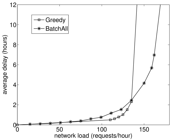
Figure 5: Performance comparison of algorithms $\mathtt{BatchAll}$ and $\mathtt{Greedy}$ for the 8-node clique and Pareto file size distribution.

Figure 6 compares the performance of the $\mathtt{BatchAll}$ and $\mathtt{BatchLim}$ algorithms. The file size distribution is exponential. The figure shows that $\mathtt{BatchLim}$ is less efficient than $\mathtt{BatchAll}$ in terms of average delay, especially at low load. This result is somewhat expected given that $\mathtt{BatchLim}$ uses a less efficient batching process and its delay ratio is looser. However, since $\mathtt{BatchLim}$ is throughput optimal, its performance approaches that of $\mathtt{BatchAll}$ at high load.

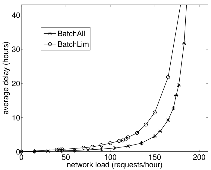
Figure 6: Performance comparison of algorithms $\mathtt{BatchAll}$ and $\mathtt{BatchLim}$ for the 8-node clique and exponential file size distribution.

Figure 7 evaluates and compares the performance of the $\mathtt{BatchAll}$ and $\mathtt{BatchAllDisp}$ algorithms. For $\mathtt{BatchAllDisp}$, results are presented for the cases where the path dispersion bound is set to either 1, 3, or 5 paths per connection. The file size distribution is exponential. The figure shows also a fluid bound on capacity derived in [26]. Its value represents an upper bound on the maximum network load for which the average delay of requests is still bounded.

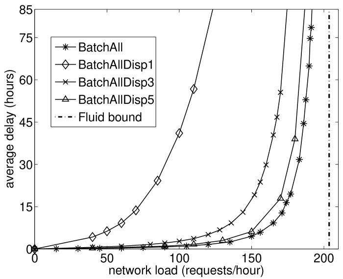
Figure 7: Performance evaluation of algorithms $\mathtt{BatchAll}$ and $\mathtt{BatchAllDisp}$ with bounds 1, 3 or 5 paths per connection for the 8-node clique and exponential file size distribution. A fluid bound on capacity is also depicted.

The figure shows that $\mathtt{BatchAll}$ approaches the capacity bound at a reasonable delay value and that a path dispersion of $5$ per connection (corresponding to $\alpha=0.089$) is sufficient for $\mathtt{BatchAllDisp}$ to achieve performance close to $\mathtt{BatchAll}$. It is worth mentioning that, in this topology, there exist $1957$ possible paths between any two nodes. Thus, with 5 paths, $\mathtt{BatchAllDisp}$ uses only $0.25\%$ of the total paths possible. The figure also demonstrates the importance of multi-path routing: the performance achieved using a single path per connections is far worse.

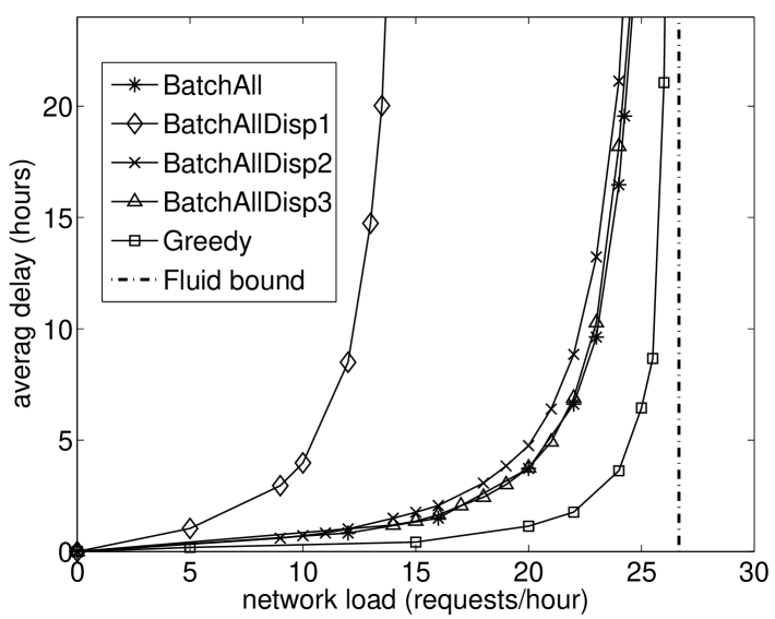
Figure 8: Performance evaluation of algorithms $\mathtt{BatchAll}$, $\mathtt{BatchAllDisp}$ and $\mathtt{Greedy\_shortest}$ for the 11-node topology 4(b) and Pareto file size. Algorithm $\mathtt{BatchAllDisp}$ is plotted with bounds of 3, 2 and 1 on path dispersion.

Figure 8 depicts the performance of the various algorithms and the fluid bound for the 11-node topology of figure  4(b). The file size follows a Pareto distribution. In this case, we observe that $\mathtt{BatchAllDisp}$ with as few as 3 paths per connection (or $\alpha=0.107$) approximates $\mathtt{BatchAll}$ very closely. Since this network is sparser than the previous one, it is reasonable to obtain good performance with a smaller path dispersion. Another observation is that for this topology and the range of network loads under consideration, $\mathtt{Greedy}$ outperforms $\mathtt{BatchAll}$ in terms of average delay. Although $\mathtt{BatchAll}$ achieves the optimal saturation throughput, its superiority over $\mathtt{Greedy}$ may only happen at very large delays. The advantage of $\mathtt{Greedy}$ in this scenario can be explained by the sparsity of the underlying topology. Seemingly, the added efficiency in throughput achieved with batching is not sufficient to compensate the cost incurred by delaying requests.

VII Conclusion

Advance reservation of dedicated network resources is emerging as one of the most important features of the next-generation of network architectures. In this paper, we have made several advances in this area. Specifically, we have proposed two new on-line algorithms for advanced reservation, called $\mathtt{BatchAll}$ and $\mathtt{BatchLim}$, that are guaranteed to achieve optimal throughput performance. We have proven that both algorithms achieve a competitive ratio on the maximum delay until job completion in $1+\varepsilon$ bandwidth augmented networks. While $\mathtt{BatchLim}$ has a slightly looser competitive ratio than that of $\mathtt{BatchAll}$ (i.e., $4/\epsilon$ instead of $2/\epsilon$), it has the distinct advantage of computing the completion time of a connection immediately as a request is placed.

A key observation of this paper is that path dispersion is essential to achieve full network utilization. However, splitting a transmission into too many different paths may render a flow-based approach inapplicable in many real-world environments. Thus, we have presented a rigorous, theoretical approach to address the path dispersion problem and presented a method for approximating the maximum multicommodity flow using a limited number of paths. Specifically, while the number of paths between two nodes in a network scales exponentially with the number of edges, we have shown that throughput competitiveness up to any desired ratio factor can be achieved with a number of paths scaling linearly with the total number of edges. In practice, our simulations indicate that 3 paths (in sparse graphs) to 5 paths (in dense graphs) may be sufficient.

As shown in our simulations, for some topologies, a greedy approach may perform better than the competitive algorithms, especially at low load, in sparse topologies, or with uncorrelated traffic between different pairs. However, we have shown that there exist scenarios where greedy strategies can be highly inefficient. This can never be the case for the competitive algorithms.

We conclude by noting that the algorithms proposed in this paper can be either run in a centralized fashion (a reasonable solution in small networks) or using link-state routing and distributed signaling mechanism, such as enhanced versions of GMPLS [5] or RSVP [27]. Distributed approximations of the multicommodity flow have also been discussed extensively in the literature (see, e.g., [28, 29, 30]). Part of our future work will be to investigate these implementation issues into more detail.

References

- [1] “Network Provisioning and Protocols for DOE Large-Science Applications,” in Provisioning for Large-Scale Science Applications, N. S. Rao and W. R. Wing, Eds. Springer, New-York, April 2003, argonne, IL.
- [2] N.S.V. Rao and W.R. Wing and S.M. Carter and Q. Wu, “UltraScience Net: Network Testbed for Large-Scale Science Applications,” IEEE Communications Magazine, vol. , 2005.
- [3] R. Cohen and N. Fazlollahi and D. Starobinski, “Graded Channel Reservation with Path Switching in Ultra High Capacity Networks,” in Gridnets’06, October 2006, san-Jose, CA.
- [4] “On-demand secure circuits and advanced reservation systems,” http://www.es.net/oscars/index.html.
- [5] “Dynamic resource allocation via gmpls optical networks,” http://dragon.maxgigapop.net.
- [6] Guerin, R. A. and Orda, A., “Networks With Advance Reservations: The Routing Perspective,” in Proceedings of INFOCOM’00, March 2000, tel-Aviv, Israel.
- [7] N. Fazlollahi and R. Cohen and D. Starobinski, “On the Capacity Limits of Advanced Channel Reservation Architectures,” May 2007, proc. of the High-Speed Networks Workshop. http://people.bu.edu/staro/Starobinski-abstract.pdf.
- [8] A. Goel and M. Henzinger and S. Plotkin and E. Tardos, “Scheduling Data Transfers in a Network and the Set Scheduling Problem,” in Proc. of the 31st Annual ACM Symposium on the Theory of Computing, 1999, pp. 189–199.
- [9] M. Andrews and A. Fernandez and A. Goel and L. Zhang, “Source routing and scheduling in packet networks,” Journal of the ACM (JACM), vol. 52, no. 4, pp. 582–601, July 2005.
- [10] Y. Azar and J. Naor and R. Rom, “Routing strategies for fast networks,” in Proc. of IEEE Infocom, 1992.
- [11] B. Awerbuch, Y. Azar, A. Fiat, S. Leonardi, A. Rosen, “On-line competitive algorithms for call admission in optical networks,” Algorithmica, vol. 31, no. 1, pp. 29–43, 2001.
- [12] Erlebach, T., “Call admission control for advance reservation requests with alternatives,” ETH, Zurich, Tech. Rep. 142, 2002.
- [13] S. A. Plotkin, “Competitive Routing of Virtual Circuits in ATM Networks,” IEEE J. on Selected Areas in Communication (JSAC), vol. 13, no. 6, pp. 1128–1136, 1995.
- [14] B. Awerbuch, D. Holmer, H. Rubens, and R. D. Kleinberg, “Provably competitive adaptive routing.” in INFOCOM, 2005, pp. 631–641.
- [15] S. Leonardi, “On-line network routing.” in Online Algorithms, 1996, pp. 242–267.
- [16] A. Goel, M. R. Henzinger, and S. A. Plotkin, “An online throughput-competitive algorithm for multicast routing and admission control.” J. Algorithms, vol. 55, no. 1, pp. 1–20, 2005.
- [17] Ganjali, Y. and Keshavarzian, A. and Shah, D., “Input Queued Switches: Cell Switching vs. Packet Switching,” in Proceedings of INFOCOM’03, March 2000, san-Fancisco, CA, USA.
- [18] Weichenberg, G. and Chan, V. W. S. and Médard, M., “On the Capacity of Optical Networks: A Framework for Comparing Different Transport Architectures,” in Proceedings of INFOCOM’06, March 2000, barcelona, Spain.
- [19] E. Gustafsson and G. Karlsson, “A Literature Survey on Traffic Dispersion,” IEEE Network, vol. 11, no. 2, pp. 28–36, March-April 1997.
- [20] J. Shen and J. Shi and J. Crowcroft, “Proactive Multi-path Routing,” Lect. Notes in Comp. Sci., vol. 2511, pp. 145–156, 2002.
- [21] R. Chow and C. W. Lee and and J. C. L. Liu, “Traffic Dispersion Strategies for Multimedia Streaming,” in Proceedings of the 8th IEEE Workshop on Future Trends of Distributed Computing Systems, 2001, p. 18.
- [22] F. Shahrokhi and D. W. Matula, “The Maximum Concurrent Flow Problem,” Journal of the ACM (JACM), vol. 37, no. 2, April 1990.
- [23] T. Leighton and S. Rao, “Multicommodity max-flow min-cut theorems and their use in designing approximation algorithms,” Journal of the ACM (JACM), vol. 46, no. 4, pp. 787 – 832, November 1999.
- [24] “Coin-Or project,” http://www.coin-or.org/.
- [25] “National LambdaRail Inc.” http://www.nlr.net/.
- [26] N. Fazlollahi and R. Cohen and D. Starobinski, “On the Capacity Limits of Advanced Channel Reservation Architectures,” in Proc. of the High-Speed Networks Workshop, May 2007.
- [27] A. Schill and S. Kuhn and F. Breiter, “Resource Reservation in Advance in Heterogeneous Networks with Partial ATM Infrastructures,” in Proceedings of INFOCOM’97, April 1997, kobe, Japan.
- [28] B. Awerbuch and T. Leighton, “Improved approximation algorithms for the multi-commodity flow problem and local competitive routing in dynamic networks,” in Proceedings of the twenty-sixth annual ACM symposium on Theory of computing (STOC), 1994, pp. 487 – 496.
- [29] A. Kamath and O. Palmon and S. Plotkin, “Fast approximation algorithm for minimum cost multicommodity flow,” in Proc. of the sixth ACM-SIAM Symposium on the Discrete Algorithms (SODA), 1995, pp. 493–501.
- [30] B. Awerbuch and R. Khandekar and S. Rao, “Distributed Algorithms for Multicommodity Flow Problems via Approximate Steepest Descent Framework,” in Proceedings of the ACM-SIAM symposium on Discrete Algorithms (SODA), 2007.