Internetwork magnetic field distribution from simultaneous $1.56$ $\mu$m and $630$ nm observations

Abstract

Aims. Study the contradictory magnetic field strength distributions retrieved from independent analyses of spectropolarimetric observations in the near-infrared ($1.56$ $\mu$m) and in the visible (630 nm) at internetwork regions.

Methods. In order to solve this apparent controversy, we present simultaneous and co-spatial $1.56$ $\mu$m and 630 nm observations of an internetwork area. The properties of the circular and linear polarization signals, as well as the Stokes V area and amplitude asymmetries, are discussed. As a complement, inversion techniques are also used to infer the physical parameters of the solar atmosphere. As a first step, the infrared and visible observations are analysed separately to check their compatibility. Finally, the simultaneous inversion of the two data sets is performed.

Results. The magnetic flux densities retrieved from the individual analysis of the infrared and visible data sets are strongly correlated. The polarity of the Stokes V profiles is the same at co-spatial pixels in both wavelength ranges. This indicates that both $1.56$ $\mu$m and 630 nm observations trace the same magnetic structures on the solar surface. The simultaneous inversion of the two pairs of lines reveals an internetwork full of sub-kG structures that fill only 2% of the resolution element. A correlation is found between the magnetic field strength and the continuum intensity: equipartition fields ($B\sim 500$ G) tend to be located in dark intergranular lanes, whereas weaker field structures are found inside granules. The most probable unsigned magnetic flux density is 10 Mx/cm². The net magnetic flux density in the whole field of view is nearly zero. This means that both polarities cancel out almost exactly in our observed internetwork area.

1 Introduction

Solar magnetic fields as seen in magnetograms form a particular pattern outside active regions, in the so-called quiet Sun. The largest polarimetric signals are confined to the supergranular boundaries forming the photospheric network. Inside these large-scale convective cells it is possible to detect magnetic fields with a more disperse character and with smaller polarimetric signals. These areas are called the internetwork. The magnetic structures of the network can be modeled either with a flux tube model or with the MISMA hypothesis (MIcroStructured Magnetic Atmosphere, Sánchez Almeida & Landi Degl’Innocenti, 1996). Both models reproduce the observed Stokes profiles and agree on the existence of nearly vertical magnetic fields of kG strength occupying only some 10-20 % of the resolution element. Observations at $1.56$ $\mu$m (Muglach & Solanki, 1992; Lin, 1995), 525 nm (Stenflo, 1973) and 630 nm (Sánchez Almeida & Lites, 2000) give consistent results. Unfortunately, this is not the case for the internetwork, with recent studies based on high quality spectro-polarimetric data at $1.56$ $\mu$m and $630$ nm yielding contradictory results.

The first observation of Stokes V spectra of an internetwork region was carried out by Keller et al. (1994). These authors observed the pair of Fe i lines at $525$ nm and analysed four average Stokes V spectra using the line ratio technique (Howard & Stenflo, 1971). Their conclusion was that the magnetic field strength was below $1$ kG (500 G) with a probability of $95$% (68%). Later, Lin (1995) measured directly the Zeeman splitting of the Fe i line pair at $1.56$ $\mu$m to infer the magnetic field strength. He showed that the typical magnetic field strength in the internetwork was well below kG. The retrieved kG structures were correlated with network patches. A few years later, Lin & Rimmele (1999), using the same pair of infrared lines, deduced field strengths between $0.2$ and $1$ kG.

The success of the Advanced Stokes Polarimeter (Lites et al., 1993) filled the literature with works concerning the internetwork magnetism using the Fe i pair of lines at 630 nm. Most of these studies obtained that the field strength distribution at the internetwork presents a peak at kG. These kG fields, even if they occupy a small fraction of the Sun’s surface (0.1-1%), contained most of the magnetic flux of the internetwork. Applying a Principal Component Analysis (PCA) inversion, Socas-Navarro & Sánchez Almeida (2002) also recovered magnetic field strengths of the order of kG. The database for this PCA algorithm consisted of synthetic profiles generated under the MISMA hypothesis. The most surprising fact is that, analysing the same data in terms of a Milne-Eddington inversion, Lites (2002) obtained field strengths clearly below 1 kG. Using the line ratio technique, Domínguez Cerdeña et al. (2003) confirmed the presence of ubiquitous kG fields in the internetwork. They used speckle reconstructed data in order to achieve a spatial resolution of $0.5^{\prime\prime}$.

Khomenko et al. (2003) carried out the study of an internetwork region at $1.56$ $\mu$m, measuring the Zeeman splitting to deduce the magnetic field strength. These authors obtained that the internetwork magnetic field strength was well below the kG regime, with a probability distribution function that could be reproduced by a decreasing exponential with an e-folding factor of $250$ G.

From all these works, one can summarize that studies using the 630 nm or the 1.5 $\mu$m lines have led to contradictory results: the infrared lines indicate fields below 1 kG, while the visible lines indicate a dominance of kG fields. Two plausible explanations have been presented to explain such a discrepancy. One is based on the idea that visible and near-infrared observations contain incompatible information about the internetwork magnetism (Socas-Navarro, 2003; Sánchez Almeida et al., 2003). The other suggests that the line pair at $630$ nm is not reliable for retrieving the magnetic field strength at the internetwork (Bellot Rubio & Collados, 2003; Martínez González et al., 2006; López Ariste et al., 2006).

Socas-Navarro (2003) suggested that, if kG and sub-kG fields co-exist in the same resolution element, the visible lines would be sensitive to the kG contribution, whereas the infrared lines would trace the sub-kG structures. The explanation comes from the different sensitivity of the spectral lines to the magnetic field. According to Bellot Rubio & Collados (2003), this may be the situation in the case of having kG fields occupying $\sim$ 20% of the resolution element and sub-kG fields filling the rest. If the percentages change, the premise seems not valid anymore. However, Socas-Navarro & Lites (2004) found observational evidence indicating the coexistence of sub-kG and kG fields in the internetwork. Their analysis was based on a three-component inversion, two of the components being magnetic with fixed field strengths of 1700 and 500 G and the other one being field-free. The observations were compatible with $\sim$ 20% of the resolution element filled by the 1700 G field and the rest by the $500$ G field.

Bellot Rubio & Collados (2003) performed numerical simulations of Stokes profiles at 630 nm and at 1.56 $\mu$m, assuming a magnetic field filling 5% of the resolution element. For consistency with the results by Khomenko et al. (2003), they parameterized the field strength distribution as a decreasing exponential with a mean value of 250 G. After adding some noise (to a level of 10^-3 I_c, with I_c the continuum intensity) to the synthetic profiles and inverting them, the resulting magnetic field strength distribution retrieved from the synthetic visible data set was centered at kG. On the contrary, the distribution inferred from the synthetic infrared spectra was close to the original one. They concluded that, for a sufficiently small noise level, both infrared and visible observations should agree and retrieve the initial distribution. However, and advancing some of the results that we will show in this paper, other effects apart from the noise level make the 630 nm magnetometry unreliable. This follows from the results by Martínez González et al. (2006) that, for the present observing conditions (with magnetic flux densities of $\sim$ 10 Mx/cm², noise level of $6.5\times 10^{-5}$ I_c, spatial resolution from 0.5^′′ to 1^′′), the 630 nm pair of lines does not carry enough information to retrieve the magnetic field strength.

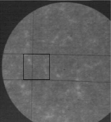
Figure 1: Ca ii K line core image from the VTT slit jaw system. Bright features are good indicators of magnetic activity. The black square marks the area scanned for this study. The lack of intense bright points in the observed area indicates a very quiet region without intense magnetic activity.

Apart from numerical simulations, simultaneous and co-spatial observations in both spectral ranges should give the final answer to the 1.56 $\mu$m-630 nm controversy. The first work with this aim was carried out by Sánchez Almeida et al. (2003) using data from the Vacuum Tower Telescope (VTT) and THEMIS telescopes at the Observatorio del Teide. This yielded two data sets in the $630$ nm and $1.56$ $\mu$m lines, but with a significantly different spatial resolution since the THEMIS telescope was not equipped with an image stabilization system at that time. The separate inversion of both data sets with a Milne-Eddington approximation led to field strengths of about $300$ G for the infrared lines and $1100$ G for the visible ones. More surprisingly, $25$% of the analysed signals showed opposite polarities in the same pixel at both wavelength ranges. Khomenko et al. (2005) showed, using magnetohydrodynamic simulations, that a different spatial resolution in both wavelengths can result in apparent opposite polarities at the same spatial point. In a subsequent publication, Domínguez Cerdeña et al. (2006) degraded the spatial resolution of the VTT data used by Sánchez Almeida et al. (2003) to match that of the THEMIS observations.From a simultaneous MISMA inversion they also obtained an important fraction of kG fields in the visible and weaker fields in the infrared. Consequently, they concluded that the information contained in the infrared data was incompatible to that contained in the visible data set. They assert that kG and weaker magnetic fields were coexisting in the resolution element, the visible being sensitive to the kG fields and the infrared to the weaker ones.

Recently, the polarimeter on-board HINODE has provided spectro-polarimetric observations at 630 nm with the highest spatial resolution ever achieved with this kind of data (0.3^′′). If the occupation fraction of the magnetic elements in the resolution element would have increased at least one order of magnitude from 1^′′ to 0.3^′′ one would have been capable of separating the effects of the thermodynamics and the magnetic field strength (Asensio Ramos et al., 2007b). Orozco Suarez et al. (2007) perform a Milne-Eddington inversion of HINODE’s data on a quiet Sun region. The noise level is around one order of magnitude higher than the one of the observations presented in this paper. In order to perform the inversions they assume one single magnetic atmosphere in the resolution element and some contamination of stray light. The retrieved magnetic field strength distribution has a peak at very weak fields, in disagreement with the previous results using the pair of spectral lines at 630 nm. However, even if this result is compatible with the magnetic fields obtained using the infrared lines at 1.5 $\mu$m, the validity of the visible spectral lines at the HINODE observational conditions should be tested.

In this work we present simultaneous and co-spatial $1.56$ $\mu$m and 630 nm observations taken at the same telescope, under very similar seeing conditions and using image stabilization systems. Spurious effects arising from a different spatial resolution in both data sets, due to different observing conditions, are thus avoided. Prior to the analysis, noise is reduced to very low values using a PCA procedure to ensure that it does not bias the study of the compatibility of the internetwork observations at these two wavelengths.

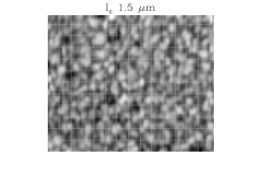
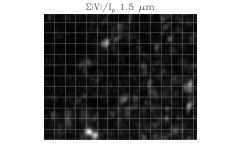
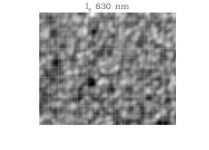
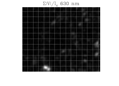
Figure 2: Maps of continuum intensity and integrated absolute circular polarization for the aligned infrared (top) and visible (bottom) data. A grid is superposed for an easier visibility of the co-spatiality of structures.

2 Observations

On August 17, 2003, a very quiet region at disc centre was observed at the VTT of the Observatorio del Teide from UT 07:34:14 to 08:26:31. A two-dimensional map was obtained by stepping the solar image perpendicularly to the spectrograph slit. At each point, the full Stokes vector was recorded at the $1.56$ $\mu$m and 630 nm spectral ranges simultaneously. The light coming from the telescope was divided using an achromatic 50% - 50% beam splitter, which sent half of the incoming radiation to the infrared polarimeter TIP (Collados, 1999) and the other half to the visible polarimeter POLIS (Beck et al., 2005b).

In order to study the internetwork, network regions or other activity areas on the solar surface were explicitly avoided with the aid of live Ca ii K images, which were accessible during the observations. The emission in the core of this spectral line is a good indicator of the magnetic activity (e.g., Lites et al., 1999). In Fig. 1 the observed region as seen in the Ca ii K line is shown. The black square contains the scanned area and the vertical line inside it represents the position of the slit at a given time. There were no intense bright zones in the whole scanned region, indicating that there was no significant magnetic activity. The size of the scanned area was 33.25^′′ (along the slit) $\times$ 42^′′ (along the scan direction). The image was stabilized using a correlation tracker system (Ballesteros et al., 1996), which allowed accurate stepping by 0.35^′′. The sampling of the spectral images was 0.35^′′ $\times$ 29.6 mÅ at 1.56 $\mu$m and 0.14^′′ $\times$ 14.9 mÅ at 630 nm. The integration time at each slit position was around 27 s. The slit widths corresponded to 0.35^′′ for TIP and 0.48^′′ for POLIS. The spatial resolution was estimated to be about 1.2^′′ and 1.3^′′ in the infrared and visible spectral ranges, respectively. The continuum contrast of the granulation were $1.3$% (infrared) and $2.7$% (visible).

3 Data reduction

Dark counts subtraction, flat-field correction and polarimetric demodulation were performed with software packages available for both instruments. Most of the instrumental polarisation crosstalk was removed using calibration optics located before the beam splitter (Schlichenmaier & Collados, 2002). For a complete correction, the coelostat configuration of the telescope needs to be modeled (Collados, 1999; Beck et al., 2005a). The residual crosstalk from Stokes I to Stokes Q, U and V was removed as:

$$\bf{P^{\prime}}=\bf{P}-\gamma I,$$ (1)

being $\bf{P}$ or $\bf{P^{\prime}}$ either Stokes Q, U or V. The symbol $I$ accounts for the intensity profile. The $\gamma$ coefficient is obtained by forcing the continuum of the polarization profiles to zero since we do not expect continuum polarization due to the Zeeman effect. Then, $\gamma$ can be computed as:

$$\gamma=\frac{P_{c}}{I_{c}},$$ (2)

being $P_{c}$ and $I_{c}$ the values the continuum of the Stokes Q, U or V profiles and of the intensity profiles, respectively. The residual crosstalk between Stokes Q, U and V is very difficult to remove. Mainly in the 630 nm data, a few percent may still remain.

After this standard data reduction, two key items still remained to correct for a precise and reliable analysis: the differential refraction of the Earth’s atmosphere and the noise level.

Differential refraction and data alignment

The differential refraction of the Earth’s atmosphere leads to a time-dependent spatial displacement of the solar images in different wavelengths, whose amount and direction depend on the combined geometrical/optical configuration of the telescope and instruments (Reardon, 2006). We already tried to minimise refraction effects during the observations by manually moving the POLIS scan mirror correspondingly in-between exposures. In order to correct for the residual differential diffraction, the continuum images of both spectral ranges were aligned. To that aim, the continuum intensity map from TIP data was divided into 24 small slices with a size of $33.25^{\prime\prime}\times 1.75^{\prime\prime}$. The POLIS continuum image was divided into slices of $45.64^{\prime\prime}\times 1.75^{\prime\prime}$. The correlation coefficient $r(d_{x},d_{y})$, for integer pixel displacements, was calculated as

$$r(d_{x},d_{y})=\frac{\sum_{ij}[A_{T}(i+d_{x},j+d_{y})-\overline{A_{T}}][A_{P}(i,j)-\overline{A_{P}}]}{\sqrt{\sum_{ij}[A_{T}(i+d_{x},j+d_{y})-\overline{A_{T}}]^{2}}\sqrt{\sum_{ij}[A_{P}(i,j)-\overline{A_{P}}]^{2}}},$$ (3)

where $\overline{A_{T}}$ and $\overline{A_{P}}$ are the average intensities of the matching areas between the TIP and POLIS slices, respectively, and $d_{y}$ and $d_{x}$ denote displacements along and perpendicular to the slit, respectively. The position of maximum correlation coefficient gives the required displacement to have co-spatial granulation maps. These displacements inferred from the continuum images were then used to retrieve the co-spatial spectra at each pixel. The displacement perpendicular to the slit was always smaller than $0.6^{\prime\prime}$. Figure 2 shows the aligned maps. It is clear that each recognisable feature is located at the same position in both the $1.56$ $\mu$m and the $630$ nm continuum intensity (or Stokes V) map.

Noise level

The noise level reached during the observations was $2\times 10^{-4}$ and $2.5\times 10^{-4}$ I_c for the $1.56$ $\mu$m and 630 nm data, respectively, with I_c being the mean continuum intensity. This noise level is typical for spectro-polarimetric data. The expected signals for internetwork fields are however so weak ($\ll$ $10^{-3}$ I_c) that we tried to improve as much as possible the signal-to-noise ratio of our data. In order to reduce the noise level, we used a statistical de-noising procedure based on the Principal Component Analysis (PCA) (Rees & Ying, 2003). The main idea is to separate the noise contribution (or residual features from the reduction process) from the real polarimetric information as follows.

Each one of our $n$ observed profiles is assumed to be a vector of size $p$, the number of wavelength points. In principle, each observed profile would be represented by a point in a $p$-dimensional space, so that one would need $p$ parameters to fully describe it. If correlations exist between these parameters, the cloud that represents all the observed profiles in the $p$-dimensional space must be elongated in some particular directions. If the matrix $\hat{O}$ contains the $n\times p$ observed profiles, these directions of maximum correlation can be obtained by diagonalising the correlation matrix of the observations (Casini & López Ariste, 2003), defined as follows:

$$\hat{X}=\hat{O}^{t}\cdot\hat{O},$$ (4)

where $\hat{X}$ is the $p\times p$ correlation matrix, the operator $\cdot$ indicates the matrix product and $t$ denotes matrix transposition. The eigenvectors of the correlation matrix form a suitable basis in which the observations can be decomposed as follows:

$$\hat{C}=\hat{O}\cdot\hat{B},$$ (5)

being $\hat{C}$ the $n\times p$ coefficient matrix and $\hat{B}$ the $p\times p$ matrix containing the eigenvectors of the correlation matrix. Each $C_{ij}$ is the projection of the $i$-th observation on the $j$-th eigenvector.

The election of this basis (the principal components) is not casual. The correlation matrix is constructed from solar profiles and the eigenvectors may have a physical meaning (Skumanich & López Ariste, 2002). However, the most important property of the PCA decomposition for our purposes is that, sorting the eigenvalues in descending order by their value, their magnitude rapidly decreases. This means that the first few eigenvectors contain the majority of the information. Under the assumption that the relevant information is contained in the eigenvectors with higher eigenvalues, the PCA basis can be truncated and those eigenvectors with small eigenvalues can be eliminated. With this, one ends up with a set of $p^{\prime}$ eigenvectors that contain mainly useful solar information. The data can be reconstructed as

$$\hat{O}_{\mathrm{filt}}=\hat{C^{\prime}}\cdot\hat{B^{\prime}}^{-1},$$ (6)

where $\hat{O}_{\mathrm{filt}}$ is the $n\times p$ matrix with the filtered data set, $\hat{C^{\prime}}$ is the $n\times p^{\prime}$ coefficient matrix and $\hat{B^{\prime}}$ is the $p\times p^{\prime}$ pseudo-basis matrix that contains only the $p^{\prime}$ first eigenvectors. The de-noising procedure is very easy, but the election of the new basis to represent the data set is a tricky point. In an ideal case, one is dealing with spectro-polarimetric information contaminated by an additive noise. In this situation, the PCA decomposition separates perfectly the noise and the real information, giving the smaller eigenvalues to the eigenvectors dominated by noise. In a real case, there exist unfortunately some other sources of noise (for instance, interference fringes, cross-talk from one polarisation state to the others, bad pixels, residual features of telluric lines on the polarization profiles, etc). All these contributions to the observed spectra have some kind of pattern and are not compatible with uncorrelated noise. The fact that they present clear patterns means that sometimes those spurious signals appear mixed with spectro-polarimetric information with non-negligible eigenvalues. Thus, the election of the new basis partly has a subjective character. We kept only the first 16 eigenvectors for the 1.5 $\mu$m data and the 31 first ones for the 630 nm data. In both cases the eigenvalues of the rejected profiles are more than 3 orders of magnitude smaller than the maximum eigenvalue. Recently, Asensio Ramos et al. (2007c) have proposed a numerical procedure to find the optimum number of eigenvectors for such kind of problem. Our selection of the reduced basis is in agreement with their calculations.

Figure 3: Top panel: circular polarization amplitude of the 1564.8 nm line (solid line) and the 630.25 nm one (dashed line). Middle panel: linear polarization amplitude for the same spectral lines. Bottom panel: ratio of the circular and linear polarization amplitudes for the same spectral lines.

Figure 4: Histograms of the amplitude (left) and area (right) asymmetries of the two-lobed Stokes V profiles at $1.5648$ $\mu$m (solid line) and at 630.2 nm (dashed line).

After applying this procedure, a filtered set of spectra with a very low noise level is obtained. The Stokes V profiles show noise values of $4\times 10^{-5}$ and $7\times 10^{-5}$ I_c at $1.56$ $\mu$m and 630 nm, respectively. The noise in the linear polarization spectra is $10^{-4}$ I_c in both data sets.

4 Analysis of polarization profiles

4.1 Amplitude of circular and linear polarization

In this section we focus on the study of directly measurable polarimetric quantities: the amplitudes of circular and linear polarization as well as the amplitude and area asymmetries of the Stokes V profiles. Interestingly, 92.6% of the observed area showed signals above three times the noise level, indicating that the whole surface is full of magnetic fields. However, in order to make a reliable analysis we selected those profiles that fulfill, simultaneously in both spectral ranges, the requirement that the maximum total polarization degree is larger than $10\sigma$, with $\sigma$ the standard deviation of the noise level at continuum wavelengths. This translates into $4\times 10^{-4}$ for the infrared and $7\times 10^{-4}$ I_c for the visible. In order not to bias our results, the amplitude of total polarization $A_{p}$ was computed for the line with less magnetic sensitivity in each spectral range (1.5652 $\mu$m and 630.15 nm) as the maximum of $\sqrt{Q^{2}+U^{2}+V^{2}}$. This gives 56.4% of the field of view with total polarization signal over the $10\sigma$ threshold.

Although the profile selection was carried out with the spectral lines with the weakest signals, we computed the amplitudes of circular and linear polarization with the lines with the largest magnetic sensitivity to the magnetic field (1.5648 $\mu$m and 630.25 nm). The amplitude of circular polarization ($A_{V}$) has been calculated as the maximum of Stokes V and the amplitude of linear polarization ($A_{L}$) as the maximum of $\sqrt{Q^{2}+U^{2}}$. Figure 3 shows the resulting histograms. The circular polarization distribution is very similar in both spectral ranges, although small differences exist. The visible lines detect slightly less weak signals than the infrared ones and slightly larger amplitudes. There is also an interesting feature common to both spectral ranges: the peak of the distributions is clearly above the noise level. One would expect that undetected weak signals (due to the noise level or to the sensitivity of the detectors) should lead to maxima of the distributions at noise level. Wang et al. (1995) studied the internetwork magnetism at a spatial resolution of $\sim$ 2^′′ using Big Bear deep magnetograms. They observed a magnetic flux distribution that peaked at $5\times 10^{16}$ Mx ($\sim$ 10 Mx/cm²), far from their detection threshold of $10^{16}$ Mx ($\sim$ 2 Mx/cm²). They examined seeing and selection effects on their results and concluded that they were not responsible for the peak and the consequent drop towards the smallest values of the distribution down to the detection limit. We have also performed numerical simulations to study the solar nature of this peak above the detection limit. In our case, we obtain that cancellations due to the poor spatial resolution produce a similar drop towards the detection limit. This means that the observed peak well above the noise level might be an observational evidence of cancellations in the resolution element.

The linear polarization histograms show very different distributions in the two spectral ranges. The visible lacks many of the signals that are detected in the infrared. Of importance is to note that the Stokes Q and U signals observed in the infrared present amplitudes that are of the same order of magnitude as those found in Stokes V. The peak of the visible distribution of $A_{L}$ is close to the noise level of $10^{-4}$ I_c, and almost no signal is detected for values of $A_{L}$ above $10^{-3}$ I_c, just the value for which the infrared distribution reaches its maximum. The infrared distribution clearly presents a peak for values much higher than the $3\sigma$ level, as already found for the amplitude of circular polarization.

In order to shed some light into the previous results, it is interesting to recall the quantities introduced by Landi degl’Innocenti & Landolfi (2004) that give an idea of the sensitivity of a spectral line to the circular and linear polarization. These quantities are defined as:

$$s_{V} = \frac{\lambda}{\lambda_{ref}}\overline{g}d_{c}$$

$$s_{L} = \left(\frac{\lambda}{\lambda_{ref}}\right)^{2}\overline{G}d_{c},$$ (7)

where $s_{V}$ and $s_{L}$ are the circular and linear polarization sensitivity index, respectively. The symbol $\lambda_{ref}$ stands for a reference wavelength. Consequently, these numbers have only sense when comparing two different spectral lines. The symbol $\overline{g}$ stands for the effective Landé factor of the transition and $d_{c}$ is the central depression in terms of the continuum intensity:

$$d_{c}=\frac{I_{c}-I(\lambda_{0})}{I_{c}},$$ (8)

with $I(\lambda_{0})$ being the intensity at the minimun of the line minimum. The symbol $\overline{G}$ plays the same role as the effective Landé factor but for linear polarization. It is defined as:

$$\overline{G}=\overline{g}^{2}-\delta,$$ (9)

where $\delta$ is a quantity that depends on the quantum numbers of the transition (see Landi degl’Innocenti & Landolfi, 2004). In both the 1564.8 nm and 630.25 nm spectral lines we have $\delta=0$. The ratios between the circular and linear polarization indices of the infrared and visible spectral lines are:

$$\frac{(s_{V})_{1.5\mu\mathrm{m}}}{(s_{V})_{630\mathrm{nm}}} = 1.37$$

$$\frac{(s_{L})_{1.5\mu\mathrm{m}}}{(s_{L})_{630\mathrm{nm}}} = 4.17.$$ (10)

This means that the sensitivity to the circular polarization is similar in both wavelengths but the sensitivity to the linear polarization is 4 times larger at 1.5 $\mu$m than at 630 nm. This result can explain the observed behaviour: the presence of ubiquitous linear polarization signals in the infrared and the lack of them in the visible.

The bottom panel of Fig. 3 shows the ratio of the circular and linear polarization amplitudes. The histogram of the 630.25 nm line shows a broad maximum near $\sim 3$, i.e. the majority of the circular polarization signals are 3 times larger than the linear polarization signals. The 1.5 $\mu$m histogram has a peak at $\sim 1$, i.e. the linear polarization signals are as large as the circular ones. If we compute the theoretical ratio, $s_{V}/s_{L}$, of the infrared and the visible lines, we obtain:

$$\frac{(s_{V}/s_{L})_{1.5\mu\mathrm{m}}}{(s_{V}/s_{L})_{630\mathrm{nm}}}=0.34.$$ (11)

Our observational data show a ratio between the circular and linear polarization of the infrared relative to the visible of 0.33, close to the theoretical prediction. As the formulae used are based on the weak field approximation, this indicates that the magnetic fields that give rise to the observed signals are most probably in the weak field regime. This means that the majority of the field strengths may be below $\approx 600$ G.

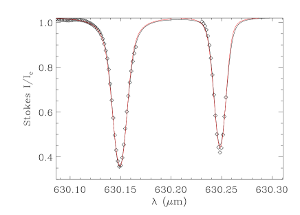
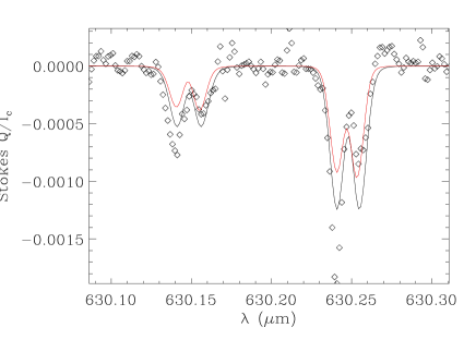
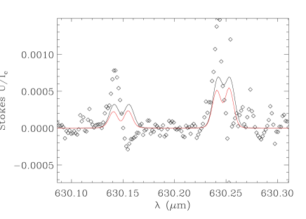
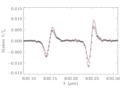
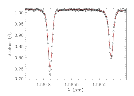
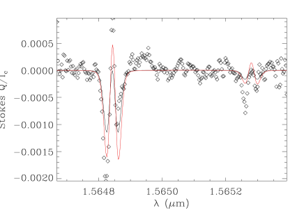
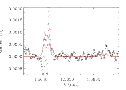
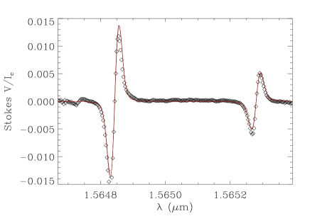
Figure 5: The four upper panels represent the four Stokes profiles of a $630$ nm observation. The four lower panels are the Stokes profiles of the co-spatial $1.56$ $\mu$m pixel. In all the plots, diamonds represent the experimental data and solid lines the best fit from the two inversion procedures: the black line shows the separate inversion and red one the simultaneous one.

4.2 Asymmetries of the circular polarization

In order to compute the asymmetries of the Stokes V profiles, we reduced the sample by selecting only those profiles that have two lobes in both spectral ranges. The procedure to find the amplitude and position in wavelength of the lobes is as follows. First, we calculated the positions where the Stokes V profile reaches zero. Then, we computed the maximum (or minimum) of the profile between two zero-crossings. With this procedure, the two spectral lines in the same wavelength range (e.g. 630.15 nm and 630.25 nm) can show a different number of lobes. To select only those lobes that are compatible in the two spectral ranges, we imposed additionally the condition that the zero-crossings have to be the same within an error of 1.7 km/s in the infrared data and 2.1 km/s in the visible data (equivalent to 3 pixels). Finally, only those profiles with two lobes in both spectral ranges were selected. With this, we ended up with 24% of the observed area. We used the definition of the amplitude ($\delta a$) and area ($\delta A$) asymmetries of Solanki & Stenflo (1984). The amplitude asymmetry is defined as:

$$\delta a=\frac{(A_{V})_{b}-(A_{V})_{r}}{(A_{V})_{b}+(A_{V})_{r}},$$ (12)

where $(A_{V})_{b}$ and $(A_{V})_{b}$ represent the amplitudes of the blue and red lobes as defined before, while the area asymmetry is defined as:

$$\delta A=\frac{A_{b}-A_{r}}{A_{b}+A_{r}},$$ (13)

where $A_{b}$ and $A_{r}$ are the absolute values of the area of the blue and red lobes, respectively. The boundaries of the integral of each lobe are different for each profile. We choose the initial point of the integration of the blue lobe as the position in the blue wing closest to the lobe which has an amplitude lower than $3\times 10^{-5}$ I_c and the ending point the zero-crossing of the profile. This last wavelength is the lower limit of the integration of the red lobe and the final one is again the wavelength point in the red wing closest to the profile having an amplitude lower than $3\times 10^{-5}$ I_c.

Figure 4 shows the histograms of the amplitude and area asymmetry. The amplitude asymmetry distributions for the visible and infrared data peak at 0.15. Both are similar in shape, but the one corresponding to the visible lines is slightly broader. The infrared distribution is very similar to that of Khomenko et al. (2003), who also found a peak at 0.15. The histograms of the area asymmetries are more symmetric than those of the amplitude asymmetries and are both centered at 0. Again, the visible distribution is broader than the infrared one. For comparison, the infrared histogram shown in Khomenko et al. (2003) peaks at 0.07 and seems to be narrower. Positive amplitude asymmetries and zero area asymmetries mean that our Stokes profiles have a higher amplitude and narrow blue lobe and a small amplitude and broad red lobe. This kind of asymmetric profiles are typical of active regions like plages and network (Solanki & Stenflo, 1984).

Figure 6: Magnetic field strength distributions at internetwork regions recovered from the separate inversion of the $1.56$ $\mu$m pair of lines (solid line) and the $630$ nm ones (dashed line) and from the simultaneous inversion of the two data sets (dotted line). The left panel shows the histogram of the magnetic field strength. The right panel represents the PDF. Both representations have been plotted to easily compare with previous works. Note that the PDF takes into account the filling factor.

Figure 7: Granular (solid line) and intergranular (dashed line) magnetic field strength distributions recovered from the separate $1.56$ $\mu$m inversion (left plot) and from the $630$ nm one (right plot).

5 Inversion of the full Stokes vector

Inversion procedures are very powerful diagnostic techniques that allow us to retrieve the physical conditions of the solar atmosphere from the information contained in the Stokes vector. However, the smaller the signal-to-noise ratio the smaller the information contained in the spectra. This was our main reason for using the PCA to reduce the noise contribution. We used the SIR code (Ruiz Cobo & del Toro Iniesta, 1992) to carry out the inversions of our data sets. We adopted a two-component model to reproduce the observed signals in each pixel: a magnetic atmosphere covering some fraction of it and a field-free one filling the rest of the surface. This modeling only allows us to reproduce regular anti-symmetric V profiles. Consequently, we only used two-lobed V profiles with a signal-to-noise ratio above $10\sigma$ in both spectral ranges.

The free parameters of the inversion for the field-free atmosphere are: the temperature height profile (with a maximum of 5 nodes), the line-of-sight (LOS) velocity height profile (with a maximum of 3 nodes) and the microturbulent velocity. Concerning the magnetic component, the parameters are: the temperature height profile (with a maximum of 5 nodes), the microturbulent and the LOS velocity, the magnetic field strength, the inclination of the magnetic field vector with respect to the LOS and the field azimuth. The magnetic field vector and the LOS velocity are set constant with height. One single macroturbulent velocity was applied to the synthetic profiles. The filling factor of the magnetic component is also a parameter of the inversion.

As a first step, we performed separate inversions of the $1.56$ $\mu$m and 630 nm data. As will be demonstrated below, since the information contained in both spectral ranges is compatible, we also carried out an inversion of both spectral ranges simultaneously.

The assumption of magnetic field properties and LOS velocities constant with height prevents the recovery of the asymmetries of the Stokes V profiles. Thus, profiles with strong asymmetries cannot be well reproduced, although other properties like the amplitude ratio between the two lines (for each pair of lines) or the width of the Stokes V lobes can be correctly fitted. Figure 5 shows examples of observed and best-fit profiles for the $1.56$ $\mu$m and 630 nm lines for the separate (black line) and the simultaneous inversion (red line). In both cases, Stokes I and V are correctly reproduced. The observed linear polarization signals are extremely low and show some crosstalk contamination (mainly at 630 nm). In spite of this, the shapes and the amplitudes of the profiles are nicely reproduced.

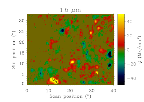
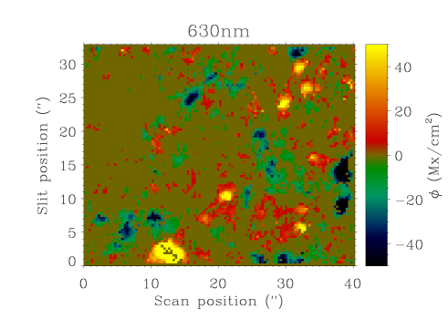
Figure 8: Magnetic flux density maps retrieved from the separate inversions of the $1.56$ $\mu$m and $630$ nm data. Both maps have been saturated to the range -50 and 50 Mx/cm².

6 Results

6.1 Magnetic field strength distributions from independent inversions of the 1.5 $\mu$m and 630 nm data sets

Figure 6 shows the magnetic field strength distributions retrieved from the separate inversion of the infrared and visible data sets (solid and dashed lines, respectively). The left panel represents the histogram of the magnetic field strength for a direct comparison with Khomenko et al. (2003). The right panel represents the probability density function (PDF) for a direct comparison with Sánchez Almeida et al. (2003). The PDF is the probability of finding a particular range of magnetic field strengths between $B$ and $B+dB$ in the field of view. It has been computed from the inversion results as:

$$PDF(B,B+\Delta B)=\frac{\sum_{i}f(B_{i},B_{i}+\Delta B_{i})}{N\Delta B},$$ (14)

where $f(B_{i},B_{i}+\Delta B_{i})$ is the value of the magnetic filling factor for the magnetic field strengths that are between $B_{i}$ and $B_{i}+\Delta B_{i}$. The symbol $N$ represents the total number of profiles in the field of view and $\Delta B$ denotes the bin size. Note that the PDF takes into account the filling factor of the magnetic elements.

The $1.56$ $\mu$m inversions reveal that the majority of magnetic fields at the internetwork have field strengths well below kG. This has been already pointed out by other works using the same pair of lines (Lin, 1995; Lin & Rimmele, 1999; Khomenko et al., 2003). It must be noted that the shape of the infrared distribution resembles that presented by Khomenko et al. (2003). On the contrary, the field strength distribution obtained from the visible lines has a peak at kG fields. This result is in agreement with the works of Socas-Navarro & Sánchez Almeida (2002), Domínguez Cerdeña et al. (2003), Sánchez Almeida et al. (2003), Lites & Socas-Navarro (2004) and Domínguez Cerdeña et al. (2006). The approximate height of formation of the infrared pair of lines is deeper than for the visible ones. However, this difference in height ($\sim 200$ km) is not big enough to explain the extremely different values of the field strength. At this point, the magnetic field strength recovered separately from the $1.56$ $\mu$m and $630$ nm inversions are apparently incompatible.

In order to check the reliability of the inferred magnetic field distributions, we study the distributions of granular and intergranular regions. The spatial resolution in our data was good enough to show a correlation between the continuum intensity and the bulk velocity, in the sense that dark areas in our data statistically correspond to downflows (intergranular lanes) and bright areas to upflows (granules). We select as granules those pixels where the continuum intensity was larger than the mean continuum intensity and intergranules those which present smaller values. Figure 7 shows the magnetic field strength distribution for granular and intergranular regions. In the infrared we can clearly distinguish two different distributions. In the granular cells, the fields are intrinsically weaker and have a distribution with a tail with an exponential decay. In the intergranular lanes, the distribution is centered at values near the equipartition field on the photosphere ($\sim 500$ G). This result is expected from magnetohydrodynamical considerations and was already pointed out by Lin & Rimmele (1999) and Khomenko et al. (2003). The scenario is very different in the visible data: we found the same distribution in granules and intergranules. This strange behaviour made us think that the inversion of the $630$ nm lines alone might not be reliable.

The magnetic filling factors inferred from the analysis of the $1.56$ $\mu$m data is $1-2$% for magnetic field strengths larger than $300$ G. Smaller field strengths are in the weak field regime and the magnetic field strength can not be separated from the filling factor. In the visible, the filling factor is $0.5-1$% for field strengths higher than approximately $500$ G.

6.2 Compatibility of the observations

In this section, we present arguments about the compatibility of our data taken at $1.56$ $\mu$m and 630 nm to be sure that the simultaneous inversion of both profiles at different wavelengths is really trustful. Some authors working mainly with the $630$ nm lines suggested that both spectral ranges carry different information about the magnetic field (Socas-Navarro, 2003). These conclusions are based on the systematical presence of opposite polarities of co-spatial circular polarization profiles at both wavelengths (Socas-Navarro & Lites, 2004). Sánchez Almeida et al. (2003) analysed simultaneous observations in both spectral ranges, discovering the presence of opposite polarities in $25\%$ of their selected profiles. Another ingredient they point out is the higher flux density inferred from visible wavelengths as compared to the one recovered from the infrared. Sánchez Almeida et al. (2003) measured an unsigned flux density at $630$ nm that was almost two times the one at $1.56$ $\mu$m.

Figure 9: Magnetic field strength distributions recovered from the inversion of the 630 nm data set with a kG (solid line) and a 200 G (dashed line) magnetic field strength initialization. The inset window represents the goodness of the fit in terms of the standard deviation of the difference between the observed and fitted Stokes V profiles.

In our simultaneous observations, opposite polarities are not a common occurrence, amounting only to $3.6\%$ of our two-lobed selected profiles. Figure 8 shows the spatial distribution of the magnetic flux density recovered from the separate analysis of the infrared and visible lines, defined as:

$$\phi=fB\cos{\theta},$$ (15)

being $\theta$ the inclination of the magnetic field vector with respect to the LOS. Both infrared and visible lines measure the same magnetic flux density, as shown by the strong correlation between both maps. Only those areas of more intense magnetic flux density are slightly larger in the visible than in the infrared. Not only the value of the magnetic flux density is compatible but also the polarities are the same in the same pixel in both spectral ranges. Consequently, the conclusion can be reached that both spectral ranges are tracing the very same magnetic features in the solar surface. The following question arises: if the observations are compatible in both spectral ranges, why does the magnetic field strength distribution at both spectral ranges seem to be incompatible?

Martínez González et al. (2006) showed that the 630 nm lines do not carry binding information about the magnetic field strength at internetwork areas. They showed that with typical present internetwork observations (magnetic flux density $\sim$ 10 Mx/cm² and a noise level of $6.5\times 10^{-5}$ I_c) the magnetic field strength can not be reliably recovered and separated from the thermodynamic parameters of the atmosphere. In order to check the reliability of the retrieved magnetic field distribution from the independent $630$ nm inversions, we perform two different inversions with two different initializations of the code: one with a kG field (the one showed in Fig. 6) and another one with an initial sub-kG field strength ($200$ G). Figure 9 shows the two inferred magnetic field distributions from the two different inversion procedures. The one starting with a kG field results in a field strength distribution with a predominance of kG magnetic fields, while the one initialized in the sub-kG regime is radically different, presenting a peak around $200$ G. The inset window shows the mismatch (in terms of the standard deviation, $\sigma$) between the observational Stokes V profiles and the fits for both initializations. Although the whole Stokes vector is well reproduced, we have only taken Stokes V into account to avoid our results to be biased by the intensity profile. All the points remain in the diagonal, meaning that indistinguishable profiles are obtained from both different inversions. Figure 10 shows the microturbulent velocity histograms of the magnetic component retrieved from the inversion of the 630 nm data set with the weak and strong initializations. As can be seen, the initialization with a weak field gives rise to larger values of the microturbulent velocity. This is used by the inversion code to broaden the profiles since the magnetic field is not strong enough. The inset window in the same figure shows the difference between the mean temperatures of the magnetic component retrieved from the weak and strong initializations. The presence of different temperatures at the (different) heights of formation of the $630.15$ and $630.25$ nm lines are used to modify the relative amplitudes of their Stokes V profiles in order to compensate for the weak value of the field strength. Consequently, since the magnetic field strength cannot be disentangled from the thermodynamics, one cannot discriminate between the two recovered magnetic field strength distributions shown in Fig. 9.

According to our results, the claim by Socas-Navarro (2003) that there is an observational bias produced by the difference in wavelength of the two spectral regions does not sustain until reliable results are found for visible lines. We have been able to obtain sub-kG or kG fields from the same data set in the visible lines. Recently, Ramírez Vélez, López Ariste & Semel (private comunication) have used the Mn i spectral line at $553.7$ nm and find results that are in agreement with those obtained from the $1.56$ $\mu$m, with a distribution of magnetic field strengths in the internetwork well below the kG regime. The observations at $1.56$ $\mu$m and 630 nm are compatible and a simultaneous inversion based on a single magnetic component does not lead to contradictions and appears to be sufficient.

Figure 10: Magnetic microturbulent velocity distributions recovered from the inversion of the 630 nm data set with a kG (solid line) and a 200 G (dashed line) magnetic field strength initialization. The inset window represents the difference between the mean temperatures of the magnetic component inferred from the weak and strong initializations.

Figure 11: Left panel: granular (solid line) and intergranular (dashed line) magnetic field strength distributions recovered from the simultaneous $1.56$ $\mu$m and $630$ nm inversions. The dotted line is the total distribution. Right panel: distribution of the magnetic filling factor.

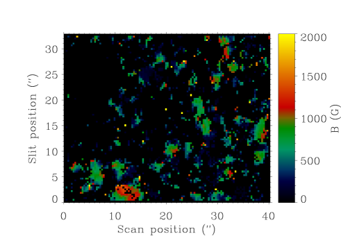
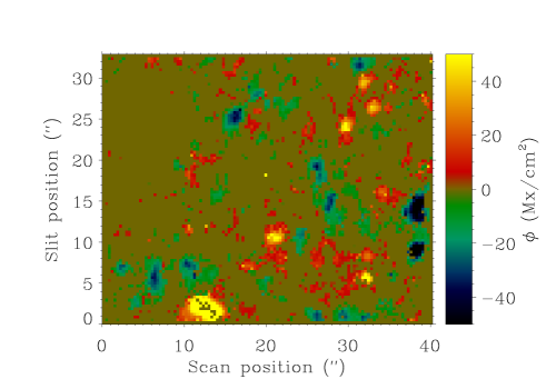
Figure 12: The left panel shows the spatial distribution of the magnetic field strength retrieved from the simultaneous inversions of the infrared and visible data sets. the right panel represents the map of the magnetic flux density. All points set to zero were not analyzed.

Figure 13: Left panel: magnetic field strength versus the inclination with respect to the LOS. Right panel: histogram of the magnetic flux density. All magnitudes have been recovered from the simultaneous inversion of the infrared and visible data sets.

Figure 14: Left panel: magnetic flux density distributions of granules (solid line) and intergranules (dashed line). Right panel: unsigned magnetic flux density distributions of granules (solid line) and intergranules (dashed line). The dotted line is the total unsigned magnetic flux distribution. All magnitudes have been recovered from the simultaneous inversion of the infrared and visible data sets.

6.3 Simultaneous inversion of infrared and visible data sets

When inverting the four spectral lines simultaneously, more physical constraints are added, leading to a larger reliability of our analysis. Figure 6 shows the magnetic field strength distribution (histogram and PDF representations) inferred from the simultaneous inversion of the two different spectral ranges (dotted line). The sub-kG field strengths dominate the magnetic field strength distribution at the internetwork. Even if the information of the $630$ nm lines has been taken into account in the simultaneous inversion, the magnetic field strength resembles substantially the one obtained with the isolated analysis of the $1.56$ $\mu$m lines.

Figure 11 shows the magnetic field strength distribution on granular and intergranular regions. Granules present a histogram that has a decreasing exponential shape with intrinsically weak fields. Intergranules, however, present a maxwellian-type behaviour centered on equipartition fields. The conclusion is, therefore, the same as that obtained from the inversion of the infrared pair of lines alone. The right panel of Fig. 11 shows the distribution of the magnetic filling factor. Most of the inferred magnetic fields fill up only $2$% of the resolution element.

The spatial distribution of the magnetic field strength is shown in the left panel of Fig. 12. The scale of variation of the magnetic field strength is $\sim 2-5^{\prime\prime}$, showing patches whose size is similar to that found for the magnetic flux density on the right panel of Fig. 12. These scales are larger than the spatial resolution and are not only due to smearing by the seeing conditions. If we compare the two maps, kG features are concentrated in few locations corresponding to the highest magnetic flux densities. On the contrary, this conclusion is not reversible, since there are strong magnetic flux density concentrations associated with hG field strengths (for instance, positions [17^′′,26^′′] and [$38^{\prime\prime}$,$14^{\prime\prime}$]). The spatial distribution of magnetic field strengths is really close to the one retrieved from the infrared inversion. Not only the simultaneous and the separate infrared magnetic field strength distributions are substantially similar, but also their spatial distributions are in very good agreement. The spatial distribution of the magnetic flux density is very similar to the one retrieved from the separate inversion. This is an interesting point since while $630$ nm lines are not capable of giving good results for the magnetic field strength, they are good indicators of the magnetic flux density.

The left panel of Fig. 13 shows the magnetic field strength as a function of the inclination of the magnetic field vector. It seems that there is a tendency for intrinsically stronger fields to be more vertical. Intrinsically weaker ones have a wider range of angles. The right panel of Fig. 13 represents the histogram of the magnetic flux density. Both polarities are equally probable in our data set. In fact, the total flux density in the field of view is $-0.055$ Mx/cm². This very small flux imbalance has been considered to point towards a $local\leavevmode\nobreak\ dynamo$ as the mechanism that generates the magnetic fields on the internetwork (Wang et al., 1995; Lites, 2002). The total unsigned flux in the field of view is $4.10$ G, something in between the figure computed from the separate infrared (2.94 Mx/cm²) and visible (4.85 Mx/cm²) inversions. Figure 14 shows the magnetic flux density (signed and unsigned) in granular and intergranular regions. There are no clear differences between the two distributions in granules or intergranules. It seems that the magnetic flux density remains the same in the whole solar surface, irrespective of the plasma motions.

7 Conclusions

Simultaneous and co-spatial observations of Fe i $1.56$ $\mu$m and Fe i $630$ nm pair of lines have been analysed. A total of 93% of the observed field of view has polarimetric signals above three times the noise level. This means that at 1^′′ spatial resolution the internetwork is full of magnetic fields.

In order to study the internetwork magnetism, the information of the full Stokes vector has to be taken into account. At this point the $1.56$ $\mu$m lines present a big advantage when compared to the 630 nm ones. Both pairs of lines are equally sensitive to the circular polarization. However, the infrared lines show conspicuous linear polarization signals while the visible ones show these signals only in few weak features.

The Stokes V profiles are quite asymmetric at both spectral ranges, having similar distributions of area and amplitude asymmetries. Most of the observed two-lobed profiles have an amplitude asymmetry of about 15% and an area asymmetry mainly zero.

We have performed the separate inversion of the infrared and visible data in order to check their compatibility. Our conclusions are:

• The magnetic flux density recovered from the independent inversion is the same at both spectral ranges (both spatial distributions have a strong correlation). Small differences can be produced by the different formation heights of the two pairs of lines.

• There are no systematic opposite polarities for co-spatial Stokes V profiles in both observations.

• The magnetic field strength distributions are very different. The infrared observations result in equipartition or even weaker fields while the visible lines show fields in the kG regime.

These three points are compatible since the validity of the magnetic field strength distributions retrieved from the 630 nm data has been questioned. We conclude that the information of our observations is compatible in both spectral ranges. This means that both the $1.56$ $\mu$m and 630 nm lines trace the same magnetic structure on the solar surface. Anyway, it does not mean that the infrared distribution of magnetic field strengths is the real one. One should keep in mind that the Zeeman effect is only capable of detecting magnetic fields in $\approx\sim$2% of the resolution element. What we really know is that our observations lead to reliable results and that the magnetic field strengths that we infer are really present on the internetwork. Ramírez Vélez, López Ariste & Semel (private comunication), with observations of a Mn i line in the visible that is sensitive to the magnetic field strength, have concluded that the magnetic field strengths on the internetwork are well below the kG regime. This supports the fact that the infrared is not biased towards weak fields.

In order to put more physical constraints, we have performed the simultaneous inversion of both data sets. The inferred magnetic field strength distribution is dominated by sub-kG fields. The occupation fraction of those fields peaks at $2$% but with a broad distribution. Two different magnetic field strength distributions are present on granules and intergranules. The granular one has intrinsically weaker field strengths than the intergranular one, which is centered on the equipartition field of the photosphere. The magnetic flux density distribution is the same on granules and intergranular lanes. There is no net magnetic flux density in the studied field of view, implying that there is a perfect cancellation of positive and negative magnetic flux density.

The unsigned magnetic flux density histograms peak at $\sim 10$ Mx/cm². Martin (1987) and Wang et al. (1995) obtained the same value using magnetograms with $2-3^{\prime\prime}$ spatial resolution. This is agreement with Lites & Socas-Navarro (2004), who show that there is no apparent increment in the magnetic flux density when improving the spatial resolution from 1 to 0.6^′′.

Since the Zeeman effect allows us to study $\sim$ 2% of the resolution element, what happens in the rest of the surface? Is it field-free? If not, which kind of magnetic fields can we find in it? Asensio Ramos et al. (2007a) show the first experimental evidence of magnetic flux cancellation at the internetwork. This supports the fact that the peak of the circular and linear polarization histograms well above the noise level is produced by cancellations in the resolution element. This means that there are still undetected magnetic fields at a spatial resolution of 1^′′ (mixed polarities or extremely weak fields). The study of the internetwork magnetism has become a very interesting field that deserves more efforts to know if it can play an important role in the solar global magnetism as claimed by Trujillo Bueno et al. (2004).