The Evolutionary History of Galactic Bulges: Photometric and Spectroscopic Studies of Distant Spheroids in the GOODS Fields

Abstract

We report on the first results of a new study aimed at understanding the diversity and evolutionary history of distant galactic bulges in the context of now well-established trends for pure spheroidal galaxies. To this end, bulges have been isolated for a sample of 137 spiral galaxies within the redshift range 0.1 $<$ z$\,<$ 1.2 in the GOODS fields. Using proven photometric techniques we determine the characteristic parameters (size, surface brightness, profile shape) of both the disk and bulge components in our sample. In agreement with earlier work which utilized aperture colors, distant bulges show a broader range of optical colors than would be the case for passively-evolving populations. To quantify the amount of recent star formation necessary to explain this result, we used the DEIMOS spectrograph to secure stellar velocity dispersions for a sizeable fraction of our sample. This has enabled us to compare the Fundamental Plane of our distant bulges with that for spheroidal galaxies in a similar redshift range. Bulges of spiral galaxies with a bulge-to-total luminosity ratio ($B/T$) $>$ 0.2 show very similar patterns of evolution to those seen for pure spheroidals such that the stellar populations of all spheroids with $M$ $>$ $10^{11}$ $M_{\odot}$ are homogeneously old, consistent with a single major burst of star formation at high redshift ($z_{f}$ $\gtrsim$ 2), while bulges with $M$ $<$ $10^{11}$ $M_{\odot}$ must have had more recent stellar mass growth ($\sim$ 10% in mass since $z$ $\sim$1). Although further data spanning a wider range of redshift and mass is desirable, the striking similarity between the assembly histories of bulges and low mass spheroidals is difficult to reconcile with the picture whereby the majority of large bulges form primarily via secular processes within spiral galaxies.

1. Introduction

The history of galactic bulges remains a key issue in studies of the origin of the Hubble sequence. Originally thought to form at high redshift through dissipationless collapse (Eggen, Lynden-Bell & Sandage 1962), their continued growth, as predicted in hierarchical models (Baugh et al. 1998), is consistent with the diversity observed in their present-day stellar populations (Wyse, Gilmore & Franx 1997). Local data alone, however, cannot distinguish between quite different hypotheses for bulge formation, including secular processes triggered by interactions and the evolution of bars (Kormendy & Kennicutt 2004; Combes 2006).

The assembly history of bulges is also central to understanding the strong correlations observed between the nuclear black hole mass and bulge properties (Magorrian et al. 1998; Gebhardt et al. 2000). The different physical scales involved in these local scaling relations represent a major theoretical challenge (Miralda-Escudé & Kollmeier 2005). As ambiguities remain even if fairly precise observations are available for local samples, an important route to understanding this puzzle lies with undertaking observations at intermediate redshift. This is especially challenging for measurement of black hole masses where the sphere of influence remains unresolved (c.f. Woo et al. 2006). However, as an alternative approach, it may be more practical to attempt to measure the growth history of the bulges in which they reside.

The arrival of deep multi-color imaging data from the Hubble Space Telescope (HST) provided the first glimpse of the photometric properties of bulges at intermediate redshift. In an early paper, Ellis, Abraham & Dickinson (2001, hereafter EAD), examined aperture colors of bulges in 68 suitably oriented isolated spirals with $I_{AB}$ $<$ 24 in the northern and southern Hubble Deep Fields (HDF). The authors found a remarkable diversity in bulge colors over the redshift range 0.3 $<$ $z$ $<$ 1 (using both spectroscopic and photometrically determined redshifts), with few as red as a passively-evolving track which matches the integrated colors of luminous spheroidal galaxies observed in the HDFs . EAD concluded that bulges have suffered recent periodic episodes of rejuvenation consistent with 15–30% growth in stellar mass since $z$ $\simeq$ 1. These conclusions were challenged by Koo et al. (2005, hereafter Koo05) who located 52 luminous ($I_{AB}$ $<$ 24) bulges in the shallower but wider field Groth Strip Survey for which a more elaborate photometric decomposition was undertaken. They found that 85% of their field sample had uniformly red colors at $z$ $\simeq$ 0.8 ($\delta(U-B)$ $\simeq$ $\pm$ 0.03), as red as present-day and distant cluster E/S0s. Only a minority (8%) showed blue rest-frame colors, most of which occurred in interacting or merging systems.

In the interim, much has been learned about the luminosity dependence of evolution in the field spheroidal galaxy population. Treu et al. (2002), van Dokkum & Ellis (2003), Treu et al. (2005a&b, hereafter T05), van der Wel et al. (2005), and di Serego Alighieri et al. (2005) have undertaken comprehensive Fundamental Plane (FP) analyses of several hundred field galaxies to $z$ $\simeq$ 1. Whereas the most luminous spheroidal galaxies studied support the long-held view of early collapse and subsequent passive evolution (e.g. Bower, Lucey, & Ellis 1992), a surprising amount of recent star formation is necessary to explain the scatter and FP offsets for lower-luminosity galaxies. T05 find that as much as 20–40% of the present dynamical mass in systems with $M<10^{11}$ $M_{\odot}$ formed since $z$ $\simeq$ 1.2. For these systems, spectroscopic signatures of recent star formation are visible and several show resolved blue cores, consistent with recently-accreted gas-rich dwarfs.

The present paper aims to clarify the relationship between bulges and spheroidals in the light of the above work. The first part is motivated by the arrival of superior resolution multi-color ACS imaging data in the Great Observatories Origins Deep Survey (GOODS) fields; this represents a significant improvement over the WFPC2 data used by EAD and Koo05. The GOODS ACS dataset offers the potential of securing improved photometric parameters. In particular, EAD chose not to undertake bulge-to-disk (B/D) decomposition, arguing by example with local data (de Jong 1996) that aperture colors were adequate. In the present paper, we revisit this discussion using a larger sample with equivalently-deep but higher spatial resolution, broader wavelength coverage, spectroscopic redshifts, and employing photometric decompositions of bulge and disk parameters.

The second component is concerned with securing dynamical estimates of the bulge stellar masses from resolved spectroscopy. At intermediate redshifts, resolved spectroscopy of high quality is now possible thanks to instruments such as the Deep Imaging and Multi-Object Spectrograph (DEIMOS; Faber et al. 2003) on the Keck II telescope. Following recent progress in interpreting the mass assembly history of field spheroidals (e.g. T05), mass-to-light ratios ($M/L$) determined from FP analyses are much superior to interpretations based solely on optical colors. Our goal is to secure the mass assembly history of a representative sample of intermediate redshift bulges and to compare trends found with the integrated properties of field spheroidals.

A plan of the paper follows. In §2, we discuss the selection criteria we adopt for both the photometric and spectroscopic sample of bulges in the GOODS fields. In §3 we describe the photometric techniques used for bulge/disk decomposition, taking into account the effects of the ACS point spread function, and derive rest-frame properties (k-corrections). In §4 we compare our photometric results with earlier measures of the diversity and star formation history of intermediate redshift bulges. In §5 we describe the spectroscopic measurements undertaken with DEIMOS and their reduction to the central stellar velocity dispersions necessary to construct the FP. Key issues of disk contamination, systematic rotation, and relative aperture size are discussed. In §6 we compare the FP of bulges with the trends now well-established for more massive E/S0 galaxies. We discuss the implications of both our photometric and spectroscopic results in the context of various formation hypotheses in §7. We summarize our overall findings in §8.

Throughout this paper, for all distance dependent quantities we adopt a flat cosmological model with $\Omega_{M}$ = 0.3, $\Omega_{\Lambda}$ = 0.7, and H${}_{\hbox{\scriptsize 0}}$ = 65 km s^-1 Mpc^-1. We note that both diagnostics considered in this study – colors and evolution of mass-to-light ratios – are independent of the Hubble constant. All magnitudes are in the AB system (Oke 1974) unless otherwise noted.

2. Data

The primary dataset for this study is the GOODS public v1.0 data release (Giavalisco et al. 2004) which provides deep imaging in four ACS passbands: F435W ($B$), F606W ($V$), F775W ($i$), and F850LP ($z$). The depth and high resolution (0$\farcs$03/pix sampling) of the GOODS ACS photometry, allow for an examination of the structure and luminosity parameters of spheroidal galaxies and, in particular, spiral galaxy bulges can be isolated from their surrounding disk. Spectroscopic data is essential both for the photometric analysis where redshifts are required to create rest-frame properties, and for the FP analysis where precise bulge stellar velocity dispersions are required.

Spectroscopic data is drawn from two independent campaigns. The first is that of T05, who secured high signal/noise spectra of a magnitude-limited sample of isolated spheroid-dominated galaxies in the northern GOODS field with $z_{AB}$ $<$ 22.5 spanning the redshift range 0.1 $<$ $z$ $<$1.2 (see Figs. 1 & 2 of T05 for a mosaic of this sample). Precision central stellar velocity dispersions were secured for 181 of these galaxies via 1–2 night exposures undertaken with DEIMOS during 2003 April 1–5 at the Keck observatory.

The second component of our bulge sample arises from later Keck campaigns during 2004 and 2005 dedicated to increasing the spiral sample for this project. Here, we selected isolated spirals from the northern and southern GOODS fields according to visual classifications presented by Bundy et al. (2005). This sample was also limited at $z_{AB}$ $<$ 22.5 with the additional criterion of a known spectroscopic redshift from the Keck Team Redshift Survey (Wirth et al. 2004). This yielded a further target sample of 45 spirals within 0.1 $<$ $z$ $<$ 0.7. A mosaic of 3-color ACS images for this second subset is shown in Figure 1.

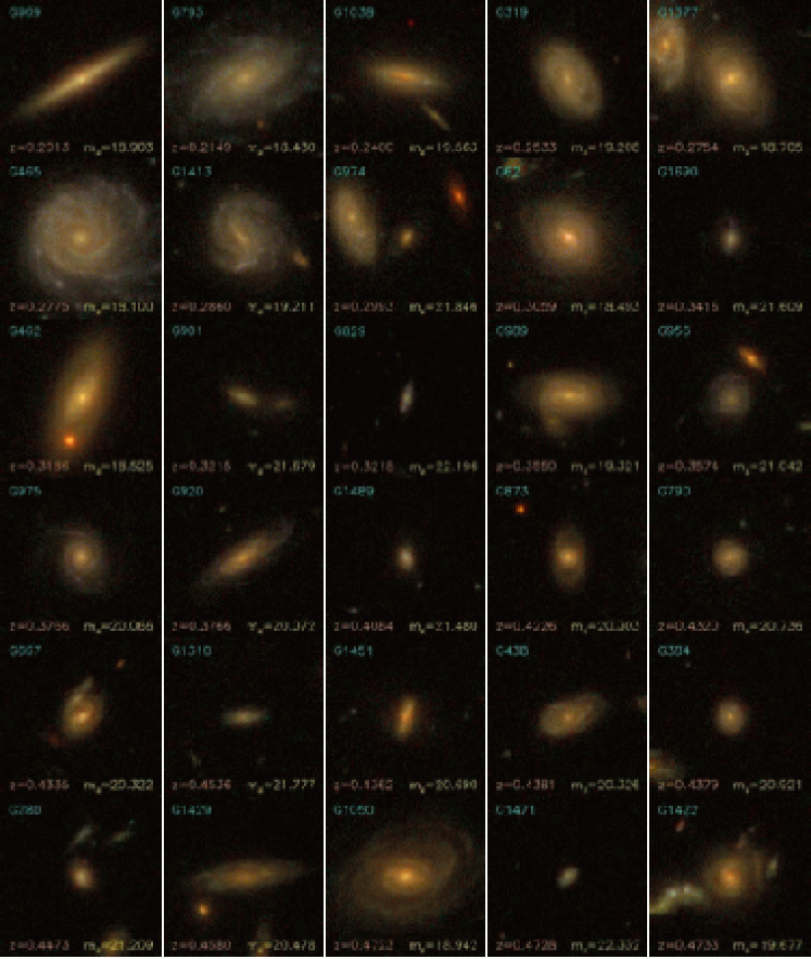
Figure 1.— Mosaic of 3-color composite ACS images (R=$z$, G=$i$, B=$V$), 7″ on a side, of the new GOODS bulge sample, sorted by redshift (lowest at top left, highest at bottom right). For each galaxy the internal ID [top left corner], redshift [bottom left corner], and total apparent $z$-band (F850LP) magnitude [bottom right corner] are indicated.

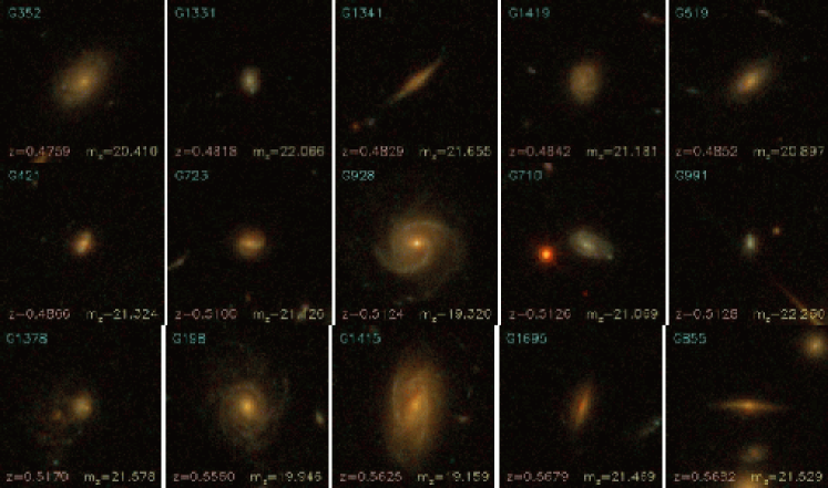
Figure 1.— Continued.

The two spectroscopic subsets are naturally somewhat different. The first, from T05, is skewed to spheroid-dominated systems considered to be E/S0s in the originally-released v0.5 images. Regardless of the original T-type classification (see T05 for details), all galaxies in the combined sample were independently visually examined as part of this analysis, in order to determine whether they were better described by 1 (pure spheroidal) or 2-component (spheroid plus disk) systems. Occasionally, particularly at high redshift, the visual inspection was not definitive. In such cases, the shape of the light profile was used as an additional guide by comparing one-component Sérsic fits to B/D decompositions (see §3.1). The different fits and their residuals were compared to single versus two-component fits of the bona-fide spirals. Since we only consider the radial component of the light profiles, the 25 high-inclination ($i$ $\gtrsim$ 70^∘) spirals in both samples are excluded from further analysis. Furthermore, a kinematic decomposition into separate components for the observed central velocity dispersion is not feasible. We thus restrict ourselves to galaxies with bulge-to-total ratio ($B/T$) greater than 0.2 for the FP analysis to ensure that the effects of disk contamination is minimal (see § 5.3). This excludes a further 21 galaxies from the recent campaign, and 25 from T05.

In summary, therefore, the photometric sample for this study comprises 193 galaxies in the redshift range 0.1 $<$ $z$ $<$ 1.2 of which 56 were modeled as single-component Sérsic profiles and 137 were decomposed into two components: exponential disk plus Sérsic bulge. The spectroscopic sample, from which the FP will be constructed, comprises 147 galaxies, 56 pure (single-component) spheroidals and the spheroidal component of 91 two-component galaxies. Eight bulges are common to both spectroscopic sub-samples, thereby offering a check on systematic errors (see § 5.2). Figure 3 shows a histogram of the redshift distributions for both the photometric and spectroscopic samples. Finally, Table A lists positions, redshifts, T-type, number of fit components, $B/T$, and total observed magnitudes (see § 3.3) for all of our sample galaxies.

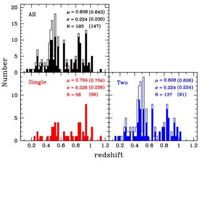
Figure 3.— Histograms of sample redshift distribution. Top: full sample; Bottom left: single component galaxies; Bottom right: two-component galaxies. Open histograms refer to the photometric sample, filled histograms and numbers in parentheses refer to the spectroscopic sample.

3. Photometric Analysis

We begin with an examination of the deep ACS images in the GOODS v1.0 data release to derive the structural and luminosity parameters of the spheroidal components (defined here as the entire galaxy for single-component galaxies, or the isolated bulge for the two-component galaxies) of the full photometric sample. A key goal is the comparison of the photometric properties of our bulges with the spheroidals analyzed by T05.

Azimuthally-averaged surface brightness (SB) profiles are extracted from the $z$-band images using the XVISTA package. Galaxy centers are determined interactively and fixed for the isophotal fit, but variable position angles (PA) and ellipticities ($\epsilon=1-b/a$, where $a$ and $b$ are respectively the semi-major and semi-minor axes) are permitted at each isophote. SB profiles are traced to $\sim$ 24–26 mag arcsec^-2 , corresponding to a systematic SB error of $\lesssim$ 0.1 mag arcsec^-2 . Profiles were extracted in at least $z$ & $i$ for each galaxy in our sample, and most $z$ $\lesssim$ 0.5 also have adequate $V$ & $B$ profiles.

3.1. Light Profile Modeling

Surface brightness profiles are modeled using techniques described in detail in MacArthur, Courteau, & Holtzman (2003, hereafter Mac03). A brief description is provided here.

Our profile modeling algorithm reduces one-dimensional (1D) projected galaxy luminosity profiles into either a single component Sérsic profile, or decomposes bulge and disk components simultaneously using a nonlinear Levenberg-Marquardt least-squares fit to the logarithmic intensities (i.e. magnitude units). Random SB errors are accounted for in the (data$-$model) minimization, whereas systematic errors such as uncertainties in the sky background and point spread function measurements are accounted for separately by performing decompositions with the nominal values as well as $\pm$ their respective errors (see § 3.2.2).

A fundamental aspect of the profile decompositions is the choice of fitting functions. The exponential nature of disk profiles has been established observationally both locally (Freeman 1970; Kormendy 1977; de Jong 1996; Mac03), and at high-$z$ (Elmegreen et al. 2005). Hence, here we model the disk light, in magnitudes, as:

$$\mu_{d}(r)=\mu_{0}+2.5\log_{10}(e){\left\{{r\over{h}}\right\}},$$ (1)

where $\mu_{0}(\equiv-2.5\log_{10}I_{0}$) and $h$ are the disk central surface brightness (CSB) and scale length respectively, and $r$ is the galactocentric radius measured along the major axis.

The appropriate form for spiral bulges and spheroidal galaxies is, however, less clear. Historically, all spheroids were modeled with the de Vaucouleurs $r^{1/4}$ profile which has proven to be a good description for the shape of luminous elliptical galaxies. However, higher resolution studies have revealed a range of profile shapes for both E/S0s and spiral bulges, which generally correlates with the luminosity (Caon et al. 1993; Andredakis, Peletier, & Balcells 1995; Courteau et al. 1996; Graham 2001; Mac03). Such a range is also supported by numerical simulations of two component (halo plus stars) dissipationless collapse (Nipoti et al. 2006) when mergers and secular evolution of disk material are accounted for (Scannapieco & Tissera 2003; Debattista et al. 2005).

To ensure the most general form for the bulge SB profile, we adopt the formulation of Sérsic, which, in magnitudes, becomes:

$$\mu_{b}(r)=\mu_{e}+2.5\log_{10}(e)\,b_{n}{\left[\left({r\over{r_{e}}}\right)^{1/n}-1\right]},$$ (2)

where $\mu_{e}(\equiv-2.5\log_{10}(I_{e}))$ is the SB at the effective radius, $r_{e}$, enclosing half the total extrapolated luminosity, and $b_{n}$ is chosen to ensure that

$$\int_{0}^{\infty}I_{b}(r)\,2\pi r\,dr=2\int_{0}^{r_{e}}I_{b}(r)\,2\pi r\,dr.$$ (3)

We use the approximation for $b_{n}$ given in Appendix A of Mac03 which is good to one part in 10⁴ for $n$ $>$ 0.36 and two parts in 10³ for $n$ $\leq$ 0.36.

It has become customary to express the disk parameters in terms of scale length and CSB ($h$ and $\mu_{0}$), while the spheroid is described in terms of effective parameters ($r_{e}$ and $\mu_{e}$). We adopt this formalism, thus parameters with subscript “$e$” refer to the bulge or spheroid. We will use a capital $R_{e}$ to indicate radii expressed in physical units (usually kpc).

For the Fundamental Plane analysis in the following sections, we also need to compute the average SB within the effective radius. For the Sérsic profile this is computed as:

$${\rm SBe}=-2.5\log_{10}(\langle I_{e}\rangle),$$ (4)

where

$$\langle I_{e}\rangle={{I_{e}\,{\exp(b_{n})\,n\,\Gamma(2n)}}\over{b_{n}^{2n}}}.$$ (5)

The best-fit parameters of the (data$-$model) comparison are then those which minimize the reduced chi-square merit function,

$$\chi^{2}_{\nu}={1\over{\rm{N-M}}}\,\,{\sum_{i=1}^{\rm{N}}}\,\left[{\mu_{gal}(r_{i})-\mu_{model}(r_{i};h,\mu_{0},r_{e},\mu_{e},n)\over\sigma_{i}}\right]^{2},$$ (6)

where N is the number of radial data points used, M is the number free parameters (i.e. N $-$ M = $\nu\equiv$ Degrees of Freedom), and $\sigma_{i}$ is the statistical error at each SB level. From here on the $\nu$ subscript will be omitted and the $\chi^{2}$ variable refers to a $\chi^{2}$ per degree of freedom.

3.2. Fitting Procedure

Constraining the five structural parameters of spiral galaxies is a challenge even at low-redshift. At higher-$z$, the lower (relative) resolution and depth limitations of the images renders the challenge even greater. In order to avoid discrepant fits between different passbands, some workers have opted to perform fits simultaneously in all bands. The scale parameters are held fixed for the decompositions in all passbands, and only the flux levels are allowed to vary to obtain colors (e.g. Koo05). This procedure implies there are no significant color gradients and that the bulge shapes are identical at all wavelengths. However, just as any morphological description of galaxies (e.g. Hubble types) depends on the wave band, intrinsic structural parameters have also been shown to vary with wavelength as a result of stellar population and dust extinction effects (e.g. MacArthur et al. 2004, hereafter Mac04). Thus, multi-wavelength information and independent fits at each wavelength are required for any accurate description of galactic structural parameters.

An additional narrowing of the parameter space is often accomplished by fixing the bulge shape to be that of a de Vaucouleurs profile (Sérsic $n$ = 4). While this may be justified for luminous spheroidal galaxies and earliest-type spiral bulges, our sample contains a range in spheroidal galaxy luminosity and extends to late-type spirals which have been shown to have bulge profiles closer to that of an exponential (e.g. Mac03), thus such a constraint would be inappropriate. Physical differences in the shape and size of spheroids among galaxies are also expected depending on how they were formed. Formation by dissipationless collapse (Nipoti et al. 2006) or accretion processes (e.g.  major/minor mergers) can account for steeply rising (high-$n$) light profiles in the central parts of galaxies (e.g.  Aguerri et al. 2001), while secular evolution of disk material (possibly triggered by a satellite) would yield shallower distributions ($n$ $\simeq$ 1–2) of the central light (Scannapieco & Tissera 2003; Eliche-Moral et al. 2006). The formation of small bulges is indeed largely attributed to secular processes and redistribution of disk material (see Kormendy & Kennicutt 2004 and references therein).

An important constraint in analyzing our present dataset is the need to compare the evolutionary characteristics of our new bulge sample with a similar sample of E/S0s (from T05). Ideally, the analysis techniques should be identical. In T05, structural homology was assumed and all profiles were modeled with a fixed $n$ = 4 profile, to conform with the standard practice for traditional studies of the Fundamental Plane of early-type galaxies in the local universe (e.g.  Dressler et al. 1987; Djorgovski & Davis 1987; Jørgensen et al. 1996). However, the goal of this paper is to extend the study to bulges, which are typically best modeled as lower $n$ Sérsic profiles. Thus, to ensure homogeneity between the analysis of bulges and spheroidals, we have re-modeled the light profiles of the T05 galaxies using Sérsic profile for the spheroid component and adding a disk component when necessary. We find a range of best fit Sérsic parameters for these early-type galaxies spanning $\sim$ 0.9 $<$ $n$ $<$ 3.4 (i.e. it does not extend as high as the de Vaucouleurs $n$ = 4 shape, see panel (d) in Fig. 6).

The following sections detail the fitting techniques which are specific to our intermediate redshift sample and are based exclusively on results from 1D B/D decompositions. The fact that we do not attempt to model non-axisymmetric shapes (bars, rings, oval distortions) lessens the need for more computationally intensive 2D B/D decompositions (extensive simulations in Mac03 showed no improvements using the 2D over the 1D decomposition method when modeling axisymmetric structures.) The measured parameters and correlations among them are discussed in §3.5.

3.2.1 Initial Estimates

In order to determine the range of best-fitted bulge and disk parameters, we need to assist the minimization program in finding the lowest possible (data$-$model) $\chi^{2}$ (c.f. Mac03). We base our initial estimates for the disk parameters $h$ and $\mu_{0}$ on a “marking the disk” technique, where the linear portion of a luminosity profile is “marked” and the selected range is fit using standard least squares techniques to determine its slope. The baseline adopted for these fits is 0.25$\,r_{max}$ to $r_{max}$. The inner boundary is chosen to exclude the major contribution of a putative bulge or a Freeman (1970) Type-II profile dip, and $r_{max}$ is the radius at which the surface brightness error is greater than 0.1 mag arcsec^-2 .

Flexibility in the bulge initial parameters is, however, limited by point spread function and sampling effects; thus the Sérsic $n$ exponent cannot be fit as a free parameter. We therefore hold $n$ fixed in the decompositions and explore the full range of 0.1 $<$ $n$ $<$ 6.0 in steps of $n$ $=$ 0.1. A grid search is performed to select the best fit. As in Mac03, for each decomposition (at fixed $n$) we explore four different sets of initial bulge parameter estimates to protect against local minima in the parameter space.

3.2.2 Point Spread Function and Sky Treatment

Bulges of late-type spirals are small and their luminosity profiles can be severely affected by the point spread function (PSF). The PSF is accounted for by convolving the model light profiles with a radially-symmetric Gaussian PSF prior to comparison with the observed profile.

The PSFs in the GOODS ACS images were estimated using a modified version of the Tiny Tim HST PSF modeling software (Rhodes et al. 2007). For each of the 4 GOODS filters, 2500 artificial stars were inserted across the ACS WFC field with a telescope focus value of $-2\,\mu$m (i.e. a primary/secondary spacing 2$\,\mu$m smaller than nominal). SExtractor (Bertin & Arnouts 1996) was then used to measure the FWHM of those PSFs. Table 1 lists the mean and standard deviation of the 2500 PSF measurements for each of the 4 ACS filters. To account for the spread in these PSF distributions, each profile is modeled with three different values of the PSF FWHM: the nominal mean value and $\pm$5% of that value.

The GOODS ACS images are already sky subtracted, so no further attempt at measuring a residual sky was made. However, we do allow for sky subtraction errors in the decompositions, in a similar manner as the PSF errors, by using three different sky levels: the measured profile as is and at $\pm$0.5% of a nominal space-based value for each band. The adopted sky levels are listed in Table 1.

The final step is to determine the best fit from the resulting 2160 decompositions. We follow Mac03 ($\S$4.3) and undertake a grid search for the minimum of two $\chi^{2}$ merit function distributions; the global $\chi^{2}$ (eq. [6]) which is dominated by the contribution from the disk, and a separate inner $\chi^{2}$ statistic computed to twice the radius where the bulge and disk contribute equally to the total luminosity ($r_{b=d}\equiv 2r(I_{b}=I_{d})$). We label this statistic as $\chi^{2}_{in}$. For cases where the bulges are so small that they never truly dominate the light profile (i.e. $r_{b=d}$ is undefined), we compute $\chi^{2}_{in}$ out to the radius at which $\nu$ = 1. Only the global $\chi^{2}$ is considered for single component fits. $\chi^{2}_{in}$ was adopted to increase the sensitivity of the goodness-of-fit indicator to the bulge area.

In cases where the bulge component is weak, fitting becomes more difficult, particularly where the rest-frame wavelength range extends into the UV for our highest-$z$ galaxies. In order to avoid unrealistically large differences in the fits between the different bands, constraints were placed based on the $i$ and $z$-band fits (where the SB profiles are closest to rest-frame $R$-band). These physical constraints are rather generous and do not contribute any subjective bias.

Figure 4 shows an example of the best fit profiles and the fit residuals derived for all four bands of the $z$ = 0.512 spiral galaxy G928. The five structural fit parameters are shown in the upper right corner, the bottom two panels show the run of ellipticity and position angle from the isophotal fits. Note that these are the same for all four bands as the $z$-band fits are used for the profile extraction of the other 3 bands.

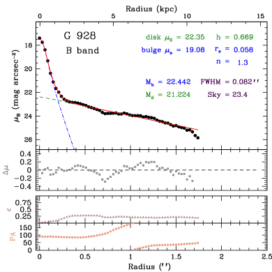
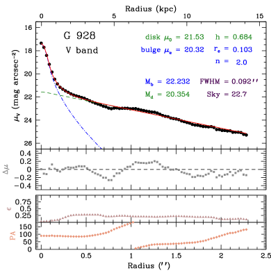
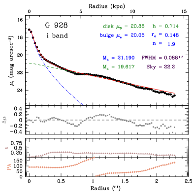
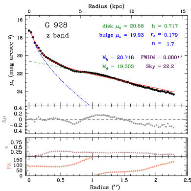
Figure 4.— Example of B/D decompositions for the $z$ = 0.512 spiral galaxy G928 in all 4 GOODS bands. In each figure, the upper panel shows the measured SB profile (solid black circles), the bulge fit (blue dashed-dotted line), the disk fit (green dashed line), and the total bulge+disk fit (solid red line). All fits are seeing-convolved using the best selected PSF values (see text). The five structural fit parameters are shown in the upper right corner, where the scales ($h$ & $r_{e}$) are in arcseconds. The second panel shows the fit residuals where $\Delta\mu(r)\equiv fit(r)-data(r)$. The bottom two panels show the run of ellipticity and position angle from the isophotal fits. Note that these are the same for all four bands as the $z$-band fits are used for the profile extraction of the other 3 bands.

3.3. Total Magnitudes and Spheroid Colors

A key goal of our study is construction of the color-redshift relation for bulges in our sample. We will thus explore in detail the relationship between the colors of the spheroidal component and those determined using apertures. We likewise wish to derive integrated magnitudes so that we can more accurately determine the bulge/total ratios implied by our photometric analysis.

Magnitudes computed involving extrapolations will be highly sensitive to the actual profile shape. For example, outer disk (anti-)truncations which are often observed in spiral galaxies would not be accounted for with a single exponential disk fit. We thus compute total galaxy magnitudes from the photometry to the maximum observed radius with the addition of the extrapolation of a linear fit to the outer 20% of the profile. The extrapolation typically increases the magnitude by $\simeq$ 0.1 mag, except when the profile is very shallow. In cases where the extrapolation adds more than 0.5 mag, the galaxy is tagged and the tabulated error is increased accordingly. We correct total magnitudes for (small) Galactic foreground extinction using the reddening values, $A_{\lambda}$, of Schlegel, Finkbeiner, & Davis (1998) and interpolating to the effective wavelength of the GOODS-ACS filters. The adopted values for both the Northern and Southern fields are listed in Table 1.

Similarly, the contribution to the total light at large radii (i.e. extrapolated to infinity) in the Sérsic profile changes significantly as a function of $n$ (see Fig. 2 of Mac03), thus a small error on the fitted $n$ could lead to an error in the total magnitude. While this error will typically not be significant for the total spheroid magnitude, the relative differences between passbands can propagate to large errors on the colors whose dynamical ranges are small (of order $\sim$ 1.5 mag for rest-frame $B-R$ and smaller for shorter wavelength baselines). To minimize the potentially large errors due to extrapolation, while still allowing for color gradients, we compute the colors of our fitted spheroids using the best fit model parameters, but only integrating out to the radius corresponding to the best fit $r_{e}$ in the $z$-band. These colors should be equivalent to aperture colors within 1 $r_{e},z$ for the single component galaxies, but can differ significantly from aperture colors for spiral bulges as they account for the (differential) contamination from disk light.

Bulge-to-total ($B/T$) luminosity ratios can be computed either from the fits alone, or as a combination of the bulge fit and the (nearly) non-parametrically measured galaxy magnitude discussed above. We adopt the latter approach as we have found that extrapolating a disk fit often overestimates its contribution.

Table 1Adopted quantities specific to the four GOODS-ACS filters

Filter	$A_{\lambda}$ (mag)		PSF (arcsec)		Sky
	North	South	$\mu$	$\sigma$	mag arcsec-2
F435W	0.0531	0.0336	0.071	0.006	23.4
F606W	0.0354	0.0233	0.080	0.006	22.7
F775W	0.0254	0.0165	0.088	0.003	22.2
F850LP	0.0165	0.0114	0.093	0.003	22.2

3.4. K-correction

The final step in deriving useful photometric quantities is the application of a $k$-correction to enable the compilation of rest-frame measures.

Often, a single function K($z$,$X-Y$), where $X-Y$ is the observed color in (optical) bands $X$ and $Y$, is derived and applied to entire samples, regardless of the galaxy type. For example, T05 provide transformations from the GOODS ACS filters to rest-frame Landolt $B$ and $V$ magnitudes (to within a few hundredths of a magnitude) for the redshift range 0 $\leq$ $z$ $<$1.25. Two filters are used in each transformation depending on where the 4000 Å break falls at the given redshift. Gebhardt et al. (2003) present a similar transformation, derived from 43 empirical SED templates, to convert from observed HST F606W and F814W magnitudes to rest-frame $U$ and $B$.

Alternatively, Blanton & Roweis (2007) provide an IDL code, kcorrect, for computing $k$-corrections which fits linear combinations of a set of model-based templates, including provision for emission lines and dust extinction, to the observed galaxy colors. kcorrect infers the underlying SEDs for galaxies over a range of redshifts by requiring that their SEDs be drawn from a similar population. The resulting reconstructed SEDs can then be used to synthesize the galaxy’s rest-frame magnitude in any bandpass.

The different methods for deriving k-corrections will have their own set of advantages and drawbacks depending on the application. As a consistency check, in Figure 5 we compare the results from all three methods mentioned above. T05 provide transformations to rest-frame $B$ and $V$ while Gebhardt et al. (2003) give transformations to rest-frame $B$ and $U$. The comparison between the three methods give reasonably consistent results for the $B$ and $V$-band k-corrections. The results are less consistent in the $U$-band. This is not surprising as it is more strongly dependent on the observed $B$-band magnitudes which have the least-well-determined profiles. An additional investigation into the templates used in the kcorrect code implies that the dust extinction prescription employed also adds to this scatter. Regardless, we can be fairly confident in the absolute $B$ and $V$ rest-frame magnitudes derived from any of the three methods for the current sample.

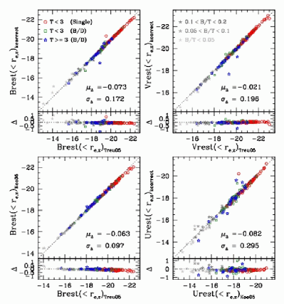
Figure 5.— Comparison of rest-frame spheroid magnitudes within the $z$-band effective radius using three different methods for deriving k-corrections: Treu05, Gebhardt et al. (2003) (also provided by Koo05 and labeled as such in the figure), and kcorrect (Blanton & Roweis 2007, see text for descriptions). Point types and colors are indicated in the upper left corners of the top panels. Gray shaded asterisks indicate galaxies with $B/T$ $<$ 0.2 which are excluded from the FP analysis in § 6. The bottom panel in each figure shows the residuals and their respective mean and standard deviations are printed in the lower right corner of the upper panels.

3.5. Structural Parameters

As a final check on our decompositions and sample characteristics, we examine here the structural parameters of our sample of spheroids with comparisons to local data. Figure 6 compares several correlations between our sample and the Mac03 sample of local bulges. The reader is advised that evolutionary effects (e.g. luminosity and/or size evolution) and selection effects (redshift dependent limiting magnitude) have the be kept in mind when interpreting these correlations and comparing them to local samples. Strong correlations are seen between luminosity and both the effective radius [panel (c)] and Sérsic $n$ parameter [panel (d)]. At a given magnitude, bulges in low-$B/T$ spirals have smaller effective radii [panel c], and there is some indication that local bulges have slightly larger $R_{e}$ at a given luminosity than those at intermediate redshift. Trujillo et al. (2006) have likewise claimed significant size evolution in the rest-frame optical for bulges in low-concentration galaxies between $z$ = 2.5 and today.

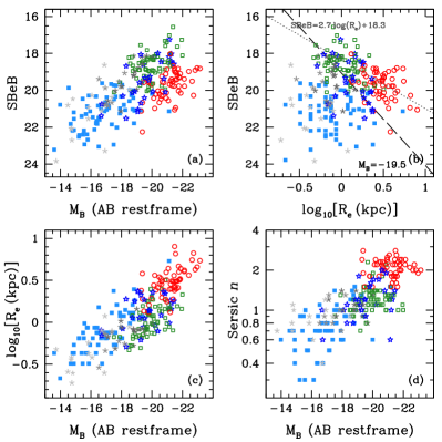
Figure 6.— Correlation of photometric parameters for the spheroidal components of our intermediate-$z$ galaxies (point types and colors are as in Fig. 5), and the local, mostly late-type, bulge sampleof Mac03 (light blue squares). The dotted line in panel (b) is a linear fit to the galaxies with M${}_{B}<-19.5$ only (i.e. the Kormendy relation for this sample) and the dashed black line is the line of constant magnitude M${}_{B}=-19.5$ (see text for discussion).

The correlation between luminosity and the effective SB within $R_{e}$ [panel (a)] is weaker and it appears that the single component Es have lower SBe for a given M_B than the spiral bulges. Graham & Guzman (2003) point out that this is a manifestation of variations in profile shape as a function of total luminosity [shown in panel (d) here and see Fig. 12 of Graham & Guzman 2003]. If one plots the central surface brightness of the bulge, $\mu(0)_{b}$ rather than SBe, the relation becomes more linear with significantly less scatter over the full luminosity range.

Finally, panel (b) plots the so-called Kormendy (1977) relation between effective radius and SBe. At first glance, there does not appear to be any correlation. However, for the most luminous spheroids with M_B $<$ $-$19.5, denoted by the dashed line, a reasonably tight relation emerges. A linear fit (dotted line) with a slope of 2.7 is in rough agreement with previously determined values (e.g. La Barbera et al. 2003 find a constant slope of 2.9 for spheroidal galaxies out to $z$ = 0.64). The difference in slope and the large scatter observed here might be expected, given the broad redshift range. Fainter spheroids deviate from this relation having smaller $R_{e}$ and/or lower SBe. The transition at M_B = $-$19.5 roughly corresponds to the luminosity below which spheroid profiles are best characterized by a Sérsic $n$ $\lesssim$ 1 (exponential) shape. Thus this represents the transition between cored ($n$ $<$ 1) and cuspy ($n$ $>$ 1) profile shapes.

Deviations in the Kormendy relation for smaller systems have been noted before in the context of differences between Es and dEs (e.g. Kormendy 1985). More recently this observation has extended to the bulges of local spiral galaxies in Ravikumar et al. (2006), who note that the fainter bulges appear more like the dEs, while the brightest bulges appear to follow the relation defined by the E/S0s. This also complies with the observation that both dEs and small bulges are more supported by rotation than their larger counterparts. The temptation to interpret the Kormendy relation as an evolutionary diagram or an indication of different formation mechanisms, however, has been disregarded due to the mixture between different types, and the changes in the profile shapes discussed above.

Prior to our photometric analysis below, we summarize in Table A our derived photometric parameters for the spheroidal components of our sample galaxies.

4. Spheroid Colors

We now turn to the first component of the analysis of our dataset which is concerned with addressing the photometric evolution of our intermediate redshift bulges. Both EAD and Koo05 presented color-redshift diagrams but using different analysis methods and different sample selection criteria. Perhaps as a result of this, they arrived at rather different conclusions. Our goal is to understand the source of any discrepancy as well as to intercompare the various approaches.

The dispersion in color at a given redshift is an important indicator of the diversity of the bulge population and hence the likelihood of continued star formation and mass assembly. Moreover, a comparison with similar data for low luminosity spheroidal galaxies will give an indication of the extent to which growth is primarily driven by processes internal to spiral galaxies.

EAD based their analysis on aperture colors (within a fixed size of 5% relative to the isophotal radius) and found that their bulges displayed a large scatter toward the blue in observed $V-I$, with few being as red as E/S0 counterparts at a given redshift. They concluded that bulges underwent recent periods of growth and associated rejuvenation. However, it is possible that the blueward scatter arises, in part, from disk contamination. As we have undertaken careful decomposition of the light profiles with the improved ACS data, here we examine the equivalent color trends with redshift for our sample.

4.1. Comparison with Aperture Colors

Bulge colors computed from B/D decompositions are extremely sensitive to the fits themselves. To understand some of these effects, and to calibrate some of the contamination that might have affected the EAD analysis, in Figure 7 we compare our fitted bulge $V-i$ colors (measured out to 1 $r_{e}$) to the central 0$\farcs$3 aperture colors [left panel] and those of the total galaxy [right panel]. The ACS PSF is $\lesssim$ 0$\farcs$09, so the 0$\farcs$3 aperture colors should not be seriously affected by PSF mismatch between bands (which are $\Delta$(PSF) $\lesssim$ 0$\farcs$008). Bulge fits are not shown if the fit magnitudes in either band were fainter than 30 mags (as these galaxies are fundamentally bulgeless).

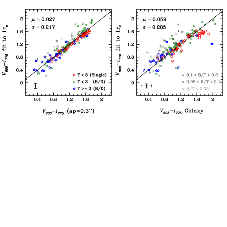
Figure 7.— Comparison of observed F606W$-$F775W ($V-i$) color from the model fits with the 0$\farcs$3 aperture color [left] and total galaxy color [right]. Point types and colors are indicated [bottom right corners] and the average errors are shown [bottom left corners]. The mean difference and standard deviation are given [top left corners] and the solid line is the one-to-one relation.

The fit and aperture $V-i$ colors are very similar, but there is some scatter such that the model fit colors are often somewhat redder than the aperture colors, particularly for galaxies that have a disk component (squares, stars, and asterisks). This probably arises from (bluer) disk contamination within the aperture. The fit colors are also often redder than the total galaxy, consistent with negative (bluing outward) gradients. Nonetheless, the above comparison confirms that our photometric decomposition is stable and yields reasonably-consistent bulge colors.

4.2. Colors vs. Redshift

We now return to the redshift dependence of our observed spheroidal component colors. Figure 8 plots the observed $V-i$ colors as a function of redshift. The black lines represent model tracks of a passively-evolving single burst population for three formation redshifts ($z_{f}$ = $0.5,1,3$) and three metallicities ($Z$ = $0.004,0.02,0.05$). All stellar population models considered are those of Bruzual & Charlot (2003, hereafter BC03). The dash-dotted cyan line is a $z_{f}$ = 3 model with solar metallicity that has extinction included using the dust models of Charlot & Fall (2000) with $\tau_{V}$ = 2 (corresponding to an $A_{B}$ $\sim$ 1.5).

As observed by many authors (e.g. T05), most of the elliptical (i.e. single component) galaxies (circles) are consistent with a single burst model with $z_{f}$ $\simeq$ 3. Those Es which deviate from this trend, indicating a more recent formation/activity, tend to be the lower-luminosity systems (as indicated by the point size). Many of the two-component galaxies (squares, stars, and asterisks) also follow this trend, but a more significant number scatter strongly to the blue and a few lie redwards of the dust-free models (even if a very high metallicity is assumed). The latter may arise from dust extinction, but the large scatter to the blue is consistent with the observations of EAD (see their Fig. 4). However, unlike EAD we do see a number of bulges that are just as red as the E/S0s. These could represent the red bulges observed by Koo05 and, indeed, if a similar cut is made on the observed $i$-band bulge magnitude as that of Koo05, the remaining spheroids in the same redshift range ($z$ $\sim$ 0.8) are red and consistent with old single-burst populations.

Thus it seems that there is no real disagreement between the studies of EAD and Koo05. While there are differences in their analysis techniques, our own internal tests suggest these are unlikely to be significant to a level that could cause such a discrepancy (§ 4.1). The fundamental difference is in the respective bulge samples: EAD sampled bulges drawn from a full range of Hubble types with the morphologically-classed spirals likely skewed towards later-type bulges. Koo05 selected bulges only from the bright end of the bulge luminosity function which, according to Figure 8, are predominantly red and passively-evolving.

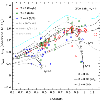
Figure 8.— Observed $V-i$ spheroid color (measured to $1\,r_{e}$ from the light profile modeling) versus redshift. Point types and colors are indicated in upper left and the point size is proportional to the rest-frame $B$ magnitude of the spheroidal component. The black lines represent BC03 models of single burst stellar populations (SSPs) formed at three redshifts ($z_{f}$ = 0.5,1,3) that evolve passively. SSPs for three metallicities are shown ($Z$ = 0.0004, 0.02, & 0.05, where $Z_{\odot}$ = 0.02). The cyan dashed-dotted line is a $z_{f}$ = 3 model with solar metallicity that has extinction included using the dust models of Charlot & Fall (2000) and $\tau_{V}$ = 2. The average error is shown as the error bar [bottom left corner].

In summary, therefore, our results confirm the diversity of bulge colors at intermediate redshift originally identified by EAD, although the bulk of the more luminous systems more closely track the relationship defined by the larger spheroidal galaxies. The question thus arises whether we are looking at two different populations each following a distinct formation path, or rather a more continuous mode of assembly for the spheroidal components where, for example, additional growth is occurring but it has proportionally less effect for the more massive systems.

Phrased another way, we can ask whether the spheroidal components of all galaxies (spirals, S0s, and Es) at a given mass are consistent in terms of their evolutionary paths. It is hard to address such a question from colors alone as the bulge luminosity or $B/T$ ratio represent poor proxies for the mass of the system. To address this more fundamental question we now turn to considering the combined set of dynamical and photometric information for our sample. By constructing the Fundamental Plane for a subset of our bulge components and comparing the relation to that now well-mapped for spheroidal galaxies of various masses (T05), we can more accurately determine the mass growth rate of luminous bulges.

5. Spectroscopic Data and Analysis

Our DEIMOS/Keck spectroscopic data are used to derive central stellar velocity dispersions which, together with the photometric parameters derived in § 3, enable us to construct the FP for the spheroidal components of E, S0, and spiral galaxies and to compare their recent stellar mass growth rates.

As discussed earlier, the spectroscopic data were taken in two distinct campaigns. The first is that described in detail in T05, relating to both E/S0s and bulge-dominated spirals. The second campaign was designed to increase the sample of spiral bulges for the current study, particularly in the redshift range 0.1 $<$ $z$ $<$ 0.7. Targets were selected with Sa+b (T=3) morphologies from Bundy et al. (2005)’s catalog to a limit of $z^{\prime}_{AB}$ = 22.5 corresponding to spirals with luminosities $-18.5$ $<$ $M_{B}$ $<$ $-20.5$.

In the following sections we describe how the new spectroscopic observations were undertaken and discuss the extraction of central velocity dispersions in the context of the earlier work by T05.

5.1. Observations & Data Reduction

The spectroscopic observations used here were taken with the Deep Imaging and Multi-Object Spectrograph (DEIMOS) on the Keck II Telescope. The data set comprises a total exposure time of 5 – 7 hours for each of 4 masks (three in the Northern GOODS field, one in the Southern GOODS field) spanning three observing campaigns in March 2004, December 2004, & March 2005. A further campaign on GOODS-S in October 2005 was unsuccessful due to bad weather and yet another campaign scheduled in October 2006 was canceled due to a major earthquake which ceased all observatory operations. Most of the data was obtained in seeing conditions in the range of 0.8–1.0″ (FWHM).

We used the 1200 line gold coated grating blazed at 7500 Å and centered at 8000 Å, which offers high throughput in the red, a pixel scale of 0$\farcs$1185 $\times$ 0.33 Å and a typical wavelength coverage of 2600 Å. A resolution of $\sim$ 30 km s^-1 was determined from arc lines and sky emission lines for the 1″-wide slitlets. In deriving velocity dispersions, the resolution was measured independently for each slit as discussed below.

The raw spectra were reduced using the DEIMOS reduction pipeline as developed by the DEEP2 Redshift Survey Team (Davis et al. 2003). After extracting one-dimensional sky-subtracted spectra, we estimated the redshift and spectral type for each galaxy. Zspec, an IDL-based software package also written by the DEEP2 Team, was used to evaluate the accuracy of the assigned redshift and a quality criterion $q$ ($-$1 for stars, 2 for possible, 3 for likely, and 4 for certain) was assigned. All spectra in our sample have a redshift quality $\geq$ 3 and most have $q$ = 4.

Noting that the minimum S/N/Å ratio for accurate central dispersions (hereafter $\sigma_{0}$) is $\gtrsim$ 10 (see, e.g., Treu et al. 2001), coupled with the desire to extract radial kinematic profiles, the spectra were coadded in radial bins to ensure a minimum S/N/Å of 5. Failure to obtain accurate $\sigma_{0}$ measurements occurred due to low S/N spectra, bad sky subtraction, unfortunately placed absorption features with respect to the atmospheric A&B absorption bands, or bulges whose velocity dispersions probably lie below our resolution limit ($\sim$ 30 km s^-1). We detail below our methodology for deriving these dispersions.

5.2. Measuring Velocity Dispersions

The velocity dispersion and rotation profiles of our spectra were measured using the well-tested Gauss-Hermite Pixel Fitting algorithm provided by van der Marel (1994).

Prior to analysis, the 1D galaxy and template spectra are matched in rest-frame wavelength range and re-binned onto a logarithmic wavelength scale. After convolving a suitable template spectrum with Gaussian velocity profiles of various dispersions, the best-fitting dispersion for each template is found (see Fig. 9 [middle panels]). The goodness-of-fit is measured via the $\chi^{2}$ statistic, weighted by the observational errors. The parameters determined for a given spectrum include the model-to-galaxy relative line strength ($\gamma$), the mean velocity ($v$), the stellar velocity dispersion ($\sigma$), and their respective errors. An advantage of the pixel fitting technique is the ability to mask, via zero weighting, undesirable regions of the spectrum, for example those containing emission lines, gaps between CCDs, and atmospheric features.

Ideally, the template spectra should be an excellent match to the spheroid stellar population (González 1993). From our previous analysis of GOODS E/S0s (T05), we have an appropriate set of high-resolution stellar templates that range from spectral types G0III to K5III. Recognizing that one of the goals of this study is to address the conjecture that bulges contain younger stellar populations, potentially spanning a range of metallicities, in addition to the observed red giant templates, we also include a selection of 36 templates from the high-resolution synthetic spectra of Coelho et al. (2005) spanning the range T_eff = 4000–7000 K, log₁₀(g) = 15–45, [Fe/H] = $-$2.0 to $+$0.5. The best-fit template is selected primarily on the $\chi^{2}$ figure of merit, but some weight is given to the line-strength parameter $\gamma$ (which should equal unity for a perfect spectral match between galaxy and template) and the formal error of the fit parameters. Indeed, in many cases, the bulge spectra are best matched by the “younger” model template spectra.

Out of 45 spiral bulges observed in this second observing campaign, successful central dispersions were obtained for 23 galaxies. 7 had marginal measurements, 13 failed to yield dispersions, and 2 had corrupt spectra. Of the 23 galaxies with successful $\sigma_{0}$ measurements, only 8 had $B/T$ $>$ 0.2 and thus could be included in our FP sample. The velocity dispersion fits for these 8 galaxies are shown in Figure 9 [middle panels].

Finally, of the 8 galaxies observed in common in both campaigns, 5 had successful $\sigma$ measurements in both and can be compared as a consistency check. Four of the galaxies had $\delta\sigma/\sigma$ $<$ 0.08 with no systematic trend. The fifth galaxy (G928) had $\delta\sigma/\sigma$ = 0.54, but this is not surprising nor worrisome, given that the spectrum is dominated by young stellar populations and emission lines, while the measurement procedure in T05 was only appropriate for older stellar populations, starting with the choice of red giant stellar templates. We thus conclude that the measurements are consistent within the error bars, when they are comparable.

5.3. Aperture Corrections & Disk Contamination

Disk contamination could potentially present a source of uncertainty when interpreting the central velocity dispersions for these spiral galaxies as representative of the bulge component. In addition to template mismatch biases, even a modest systematic rotation might lead to an overestimated value for the smaller bulges. The spatial resolution of the observations are limited by the pixel scale (0$\farcs$1185 per pixel), the physical size of the slit width (1″) and the typical seeing FWHM during the time of the observations ($\sim$0.8–1″). As mentioned in § 2, we have limited our bulge sample to those with $B/T$ $>$ 0.2 to ensure that the bulge light dominates in the center. However, the presence of a disk could still influence the measurement and interpretation of $\sigma_{0}$.

A proper kinematic decomposition of our data into contributions from the bulge, disk, and dark halo components would require full dynamical modeling (see Widrow & Dubinsky 2005). Conceivably this could be possible for a few galaxies where we have adequately sampled kinematic profiles, but is beyond the scope of the current analysis. Our main goal is therefore to estimate the likely degree to which disk light is influencing our measurements.

For those spectra where resolved kinematic data can be extracted (see Fig. 9 [right panels]), we can attempt to estimate the disk contribution to the true bulge dispersion, $\sigma_{0,b}$ from the rotation measured across the bulge (assuming this arises entirely from disk component). We model this as

$$\sigma_{0,b}=\sqrt{\sigma_{0}^{2}-(V(r_{ap})/\sin\,i)^{2}},$$

where $V(r_{ap})$ is the velocity at 1 $r_{e}$ or at a radius of 2 pixels (at 0.1185″/pix), whichever was larger. The velocity was typically very small, with the correction factor $\sigma_{0,b}/\sigma_{0}$ ranging from 0.7–1, with a mean value of 0.95. We can also monitor the possible effects of disk contamination in the bulge spectra by considering the inner dispersion gradients. Inspection of Figure 9 [right panels] reveals that the $\sigma(r)$ profiles are largely flat within the central regions ($\lesssim$ 1 $r_{e}$). Although we do not have kinematic profiles for all galaxies, given the bulk have near face-on inclinations, we conclude contamination by a rotating disk component is not significant.

Finally, we need to standardize the aperture within which the dispersion measurement refers. Several studies have considered $\sigma$ gradients in early-type galaxies and find $\sigma_{r}/\sigma_{r_{e}}=(r/r_{e})^{\alpha}$ with $\alpha=-0.04$ to $-0.06$ (e.g. Jørgensen, Franx, & Kjaergaard 1996, Cappellari et al. 2006). For our observations, we have a fixed slit-width of 1″, the DEIMOS scale is 0.1185″ per pixel, and the effective radii of our galaxies range from 0–1″, with an average value of 0$\farcs$3. As a result, although our extracted central spectrum will be dominated by the highest SB central portion, there will be some contribution from beyond 1–2 $r_{e}$. Adopting an observed effective aperture of 0$\farcs$35, the average correction to an $r_{e}/8$ aperture using $\alpha\,=\,-0.06$ is $\sigma_{r_{e}/8}=1.16\,\sigma_{ap}$, where we have chosen the standard correction to an aperture of $r_{e}/8$ for comparison of our results with other studies. Adopting $\alpha=-0.04$ would reduce the correction factor to 1.10. Our correction takes into account the measured $r_{e}$, which has the drawback of correlating $\sigma$ and $r_{e}$, but is important given the wide range of spheroid sizes in our sample relative to the constant effective aperture of our observations.

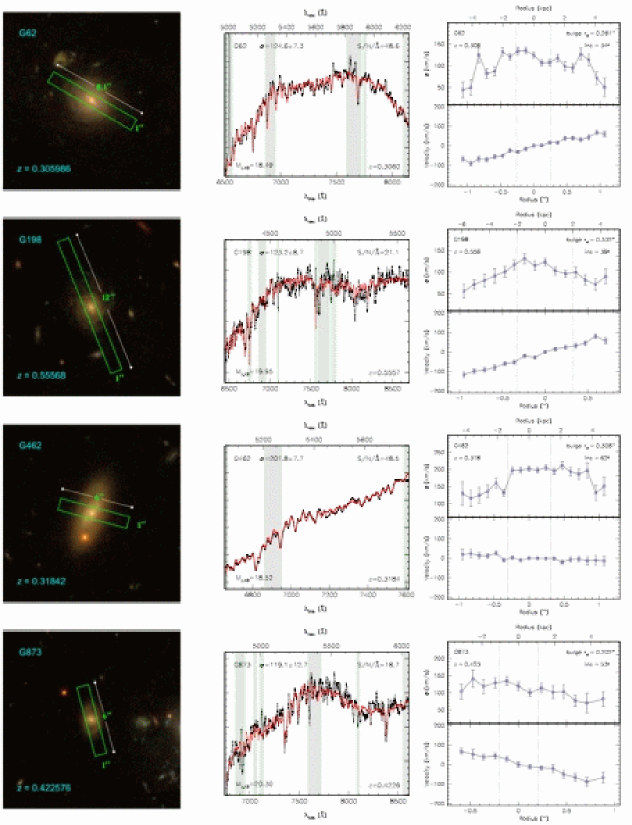
Figure 9.— Spectroscopic measurements for all galaxies from the new bulge sample with $B/T$ $>$ 0.2. Left panels: 3-color ACS image and slit orientation. Middle panels: observed central galaxy spectrum (black lines) and the best-fitting stellar template (red lines) convolved to the measured velocity dispersion. Shaded regions (flanked by vertical green lines) indicate regions masked out during the fit due to an overlap with either: A & B atmospheric absorption bands, emission lines (Balmer and [O III]$\lambda\lambda$5007,4959 Å in particular), bad regions in the stellar templates, or the gap between the blue and red spectra. The spectra have been smoothed with a 10 Å boxcar filter. Galaxy ID, $\sigma$ (in km s^-1), S/N/Å of the observation, observed $z$ magnitude, and redshift are indicated. Right panels: kinematic profiles. Top: velocity dispersion as a function of the light-weighted radius (all radial bins were coadded to S/N/Å $\geq$ 5). Bottom: radial velocity profiles (i.e. rotation curves), shifted to zero velocity at the center (determined from the peak of the spectroscopic light profile). Solid black lines connect the points to guide the eye. The vertical dashed lines are located at $\pm 1\,r_{e}$ as determined by the B/D decompositions.

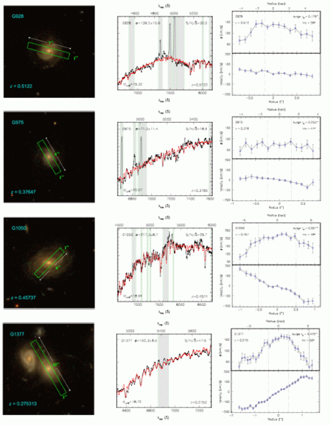
Figure 9.— Continued.

5.4. Fundamental Plane Parameters

We now use the derived photometric and kinematic parameters to construct the Fundamental Plane (FP) for our intermediate-$z$ sample of the spheroidal components of galaxies with $B/T>0.2$. The FP is traditionally expressed in terms of galaxy effective radius, $R_{e}$, the average surface brightness within the effective radius, SBe, and the central velocity dispersion, $\sigma_{0}$ (e.g. Dressler et al. 1987; Djorgovski & Davis 1987), related via:

$$\log_{10}(R_{e})=\alpha\,\log_{10}(\sigma_{0})+\beta\,{\rm SBe}+\gamma,$$ (7)

with $R_{e}$ in units of kpc, SBe in mag arcsec^-2 , and $\sigma_{0}$ in km s^-1.

In order to address the evolutionary history of mass build-up in galaxies, it is necessary to convert these measured parameters into masses and mass-to-light ($M/L$) ratios. An effective dynamical estimate of the stellar mass, $M$, can be defined using the scalar virial theorem for a stationary stellar system as

$$M\equiv\frac{c_{2}(n)\,\sigma_{0}^{2}\,R_{e}}{G},$$ (8)

where $c_{2}(n)$ is the virial coefficient. In the case of structural homology, the virial coefficient is a constant for all galaxies, thus the FP maps directly into a $M/L$ ratio (see, e.g. T05) using the usual definition for luminosity,

$$L\equiv 2\pi\,\langle I_{e}\rangle\,R_{e}^{2},$$ (9)

where $\langle I_{e}\rangle$, the average intensity within the effective radius, $R_{e}$, is given in equation (5). However, in the case of varying $n$, the profile shape does affect the measured $M/L$ through a variation in the velocity dispersion profile (even though these changes in profile shape do not significantly alter the FP or its tilt, see Fig. 11).

A number of authors have constructed spherical dynamical models to derive $c_{2}(n)$ for different profile shapes (e.g. Ciotti et al. 1996; Prugniel & Simien 1997; Bertin et al. 2002; Trujillo et al. 2004, hereafter Truj04), with generally consistent results. We use the derivation of Truj04 who constructed non-rotating isotropic spherical models, and take into account the projected velocity dispersion over an effective aperture.

For the purpose of assessing evolutionary trends, we need a local relation (at $z$ = 0) against which we can compare higher-$z$ galaxies. Ideally, one would like to have a local comparison sample that is large in numbers and homogeneous in measurement techniques to the distant sample. We are currently undergoing a major observational project at the Palomar Observatory to construct such a large, homogeneous, local sample that extends to spiral galaxies and includes both field and cluster samples (MacArthur et al., in prep).

While we await the results from that campaign, we derive a local FP comparison from a sample of early-type galaxies in the Virgo Cluster. We start from the structural analysis of Ferrarese et al. (2006) of HST images of early-type galaxies from the ACS Virgo Cluster Survey (ACSVCS) of Côté et al. (2004). Precise distance measurements come from the surface brightness fluctuation analysis of Mei et al. (2007), and velocity dispersions are carefully collected from the literature. A detailed description of our derivation of the local FP relation for Virgo cluster early-type galaxies, which relaxes the assumption of structural homology, is provided in the Appendix. The result is,

$$\log_{10}(M/L_{B})_{0}=0.225\,\log_{10}(M)-1.63,$$ (10)

and we measure the offset for galaxy $i$ from this local relation as,

$$\Delta\log_{10}(M/L)^{i}=\log_{10}(M/L)^{i}-\log_{10}(M/L)_{0}^{i}.$$ (11)

Finally, since we have not applied the usual formalism found in the literature of imposing a fixed profile shape to parametrize the light profiles, some care in the analysis and, in particular, its comparison with previous works must be taken. The correlation between the Sérsic $n$ and total luminosity seen in panel (d) of Figure 6 indicates weak homology among the spheroidal components of galaxies. This begs the question of whether this new parametrization of the light profiles has an effect on their location in the FP. To illustrate the effect of using fixed versus varying profile shapes, in Figure 11 we plot the difference between the two structural parameters entering the FP using the best fit Sérsic profile from the current analysis and the fixed de Vaucouleurs ($n$ = 4) fits from T05. The straight line is the best-fit $\log_{10}(R_{e})$ – SBe combination from the Jørgensen, Franx, & Kjaergaard (1996, hereafter J96) local relation for Coma. The E/S0s lie fairly close to the local line, indicating that the FP location of these galaxies is not strongly affected by the shape of the profile. This is due to the fact that, for a given total magnitude, a change in the shape parameter $n$ will result in a different $r_{e}$ which is compensated by a change SBe in the opposite sense. The relation is not precisely one-to-one though, but this would not be expected based on the observed evolution of the FP tilt with redshift (e.g. T05). On the other hand, there is a significant offset from the $n$ = 4 fits for the spiral bulges. This is entirely expected as T05 consider single component $n$ = 4 fits whereas we have not only allowed $n$ to vary, but we have also decomposed the profile into bulge and disk components.

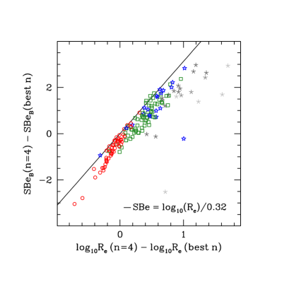
Figure 11.— Comparison of Sérsic fit parameters derived here with the T05 fixed de Vaucouleurs fits shown as the difference in SBe versus the difference in log${}_{10}(R_{e})$. Point types and colors are as in Figure 5. The solid black line delineates the combination of these parameters that enter the J96 Coma FP relation.

Table A summarizes the FP parameters derived in the preceding sections for our spectroscopic sample of 147 galaxies.

6. Spectroscopic Results

This section presents our results based on the spectroscopic sample. We first discuss the evolution of the Fundamental Plane in § 6.1 and then interpret it in terms of cosmic evolution of the mass-to-light ratio of bulges and spheroids in § 6.2. § 6.3 discusses a number of caveats that should be kept in mind through the discussion of the results and their interpretation in § 7.

6.1. Fundamental Plane Evolution

With central velocity dispersion measurements in addition to accurate photometric parameters, we now discuss the Fundamental Plane for our sample of intermediate-$z$ spheroids. In Figure 12 we show the location of our spheroids in the face-on projection of the FP plane according to the J96 local relation for Coma. We divide the sample into five redshift bins (with constant $\Delta(z)$, thus some additional scatter is expected due to the different age ranges in the different bins).

The most notable trend is that with redshift. As redshift increases, bulges and spheroids alike move further away from the local relation. This is consistent with the trend noted previously for spheroids and can be qualitatively understood in terms of the reduced age of the stellar populations. As cosmic time goes by, stars are on average older, and thus for a given size and velocity dispersion the surface brightness is lower. It is important to keep in mind when comparing with previous studies of spheroids (such as T05) that we have isolated the spheroidal component from the surrounding disk, when present. As a result, galaxies in common with T05 have generally moved downwards in size (and in luminosity). As expected, the scatter for the spiral bulges is reduced with respect to T05, because we have taken care of separating the pressure supported component from the rotation supported disk.

Looking at the trends inside each bin, the overall effect seems to imply a continuation in the FP space from the higher mass (E/S0) to the lower mass (bulge) spheroids. Also, the FP at intermediate redshift appears to be tilted with respect to the local relation. The evolution of the tilt seems to be less pronounced than that observed for spheroids considered as a single component. A confirmation and quantification of this trend awaits a larger sample.

Finally, we note that many of the smallest bulges appear to lie too far to the right of the relation defined by the bigger spheroids. While this effect could be real, we speculate that this is due to the fact that, in the case of two-component galaxies, our central velocity dispersions are sensitive to the potential from the total galaxy (bulge/disk/halo) and thus are overestimates of the “bulge-only” dispersions. This could be a partial explanation for the above mentioned apparent weaker FP tilt evolution in comparison with the pure spheroids.

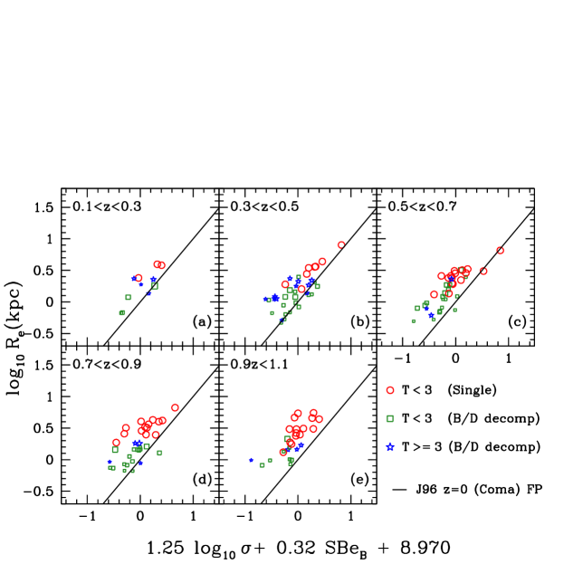
Figure 12.— Fundamental Plane of our spheroids, divided in to 5 redshift bins, with respect to an edge-on view of the FP set by the local Coma zeropoint of J96 (solid line in each panel). Point types are indicated and their size is proportional to the galaxy $B/T$ ratio.

6.2. Mass-to-Light Ratio Evolution

We now use equation (8) to derive masses for our spheroids and test some of the conjectures above of a correlation between evolutionary state with spheroid mass. In Figure 13 we plot the rest-frame $B$-band mass-to-light ratio ($M/L_{B}$; note the inverted scale on the y-axis) as a function of mass (both expressed in solar units), separated into the same redshift bins as in Figure 12. The dotted line indicates our Virgo local relation (eq. [10]) and, for comparison, the dashed line shows the J96 relation for Coma which was constructed under the assumption of structural homology. The shaded areas indicate the selection limits due to our total galaxy magnitude limit of $z_{AB}$ $<$ 22.5 mag. The more densely hatched regions correspond to the lower limit of the redshift bin, while the sparsely hatched regions are for the upper redshift limit. The gray hatches apply to the pure spheroidal galaxies and the black hatches regions are the corresponding $z_{AB}$ $<$ 24.25 limit for the two-component galaxy sample (i.e. according to our $B/T$ $>$ 0.2 limit). This selection limit imposes some restrictions on our interpretation of evolution, particularly at the highest-redshift and low-mass ends.

Several trends are noticeable upon examination of Figure 13. First, the slope of our relation is somewhat steeper than the local relation slope, and there is some indication that the steepening increases with redshift (although the latter is not conclusive due to our selection limits). Broadly speaking, it appears that the bulges follow a similar relation to that defined by the pure spheroidal galaxies. In particular, there is no evidence of an offset to lower $M/L$ ratios (due to increased $B$-band luminosity) which may be expected if the bulges are undergoing a more continuous mode of SF, as is expected in the secular formation scenario (e.g. Kormendy & Kennicutt 2004). If anything, some bulges are offset to higher $M/L$. However, as mentioned above we believe this could be due to the fact that our central velocity dispersions are sensitive to the total galaxy potential, but our derived masses are based on a formulation for the total mass of a single Sérsic profile. We may, therefore, be overestimating the mass of the spheroid for multiple-component systems. The effect does appear to be stronger for the lower $B/T$ bulges, thus strengthening the support for this hypothesis.

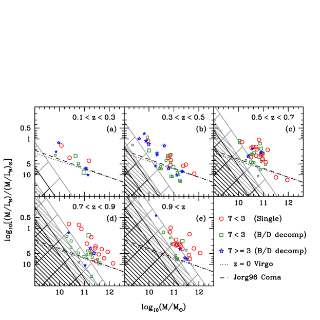
Figure 13.— $M/L$ vs. $M$ projection of the FP divided into five redshift bins. Panels and symbols are as in Figure 12. The dotted line is our Virgo local relation (eq. [10]) and the dashed line is that of J96 for Coma. Point size is proportional to $B/T$ ratio. The gray hatched regions correspond roughly to our total galaxy magnitude limit of $z_{AB}$ $<$ 22.5. The more densely hatched regions apply to the lower ends of the redshift limits while the sparsely hatched regions correspond to the upper redshift end. The black hatched regions are the corresponding $z_{AB}$ $<$ 24.25 limits on our bulges (i.e. for $B/T$ = 0.2).

Also evident in Figure 13 is that the deviation from the local relation increases as the spheroid mass decreases. We can represent this offset directly using equation (11). This is shown in Figure 14 which plots $\Delta\log_{10}\,M/L_{B}$ as a function of redshift and divided into three spheroid mass bins. This representation can be easily interpreted in terms of star formation histories in an analogous procedure to that presented in T05 (their Fig. 21). Overplotted on Figure 14 are $M/L$ evolution models from BC03. The gray lines represent a single burst of star formation at $z_{f}$ = 5 that evolves passively. The most massive spheroids (including E/S0s and bulges) in the $\log_{10}M/M_{\odot}>$ 11.5 bin are well described by this old population formed in a single burst. In the lower mass bins, however, many galaxies deviate significantly from this relation. These deviations can be explained in the context of more recent spheroid building in the form of subsequent bursts of star formation on top of an underlying old population, where the old population dominates the total stellar mass. The black lines in the two lower mass bins represent the $M/L$ evolution for such models. For the intermediate mass range (11.5 $\leq$ $\log_{10}M/M_{\odot}$ $<$ 11.0), the data are consistent with a more recent burst of SF that represents $\sim$ 5% of the total stellar mass, and in the lowest mass bin, recent bursts involving $\sim$ 10% of the total mass are required. Due to the short timescales of the initial $M/L$ decline after a burst of SF, these mass fractions are likely underestimates. These results echo those found in T05 for E/S0s.

Of particular note here is that the distribution of bulges in the representation shown in Figure 14 is largely indistinguishable from that of the pure spheroidal galaxies. Thus, we conclude that, for host systems with $B/T$ $>$ 0.2, all spheroids at a given mass appear to follow the same evolutionary path. The smaller mass spheroids – whether isolated or embedded in a disk – must have more recent stellar mass growth, so the recent observations of galaxy “downsizing” in spheroidal galaxies, both empirically (e.g. Bundy et al. 2005; T05; di Serego Alighieri et al.  2005; van der Wel et al. 2005), and in cosmological N-body + semi-analytical simulations (De Lucia et al. 2006), extends to the bulges of spiral galaxies.

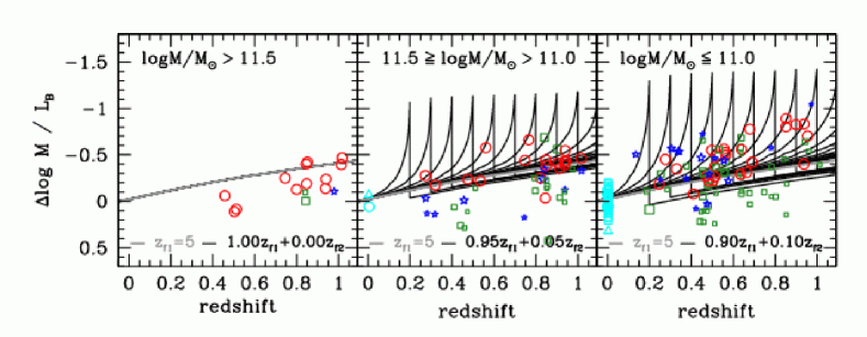
Figure 14.— Offset of $B$-band $M/L$ ratio, $\Delta\log_{10}M/L_{B}$ (eq. [11]) versus redshift and divided into 3 dynamical mass bins. Point size is proportional to $B/T$ ratio. The gray line indicates the evolutionary trend for a system that formed in a single burst at $z_{f}$ = 5 and evolves passively (from the stellar population models of BC03). Black lines illustrate the effects of secondary burst of star formation (5% or 10% by mass) at $z_{f2}$ = $0.1,0.2...$ added to the initial burst. The light blue points at $z$ $\sim$ 0 are the local Virgo galaxies (see Appendix).

6.3. Caveats

Before proceeding to a comparison of our results with other studies in the literature and to a physical interpretation of our spectroscopic and photometric results in the next section, it is important to list a number of caveats that should be kept in mind throughout the discussion.

• Most local FP comparisons are not measured in quite the same way as our distant sample. For example, $r_{e}$ is typically not computed from Sérsic fits, nor are two component fits generally applied to lenticular galaxies. This may introduce some systematic bias in our determination of the evolution of the mass-to-light ratio. For example, if the slope is steeper locally than we estimate, the deviations in Figure 14 will be tempered, and vice versa. We partially addressed this issue by compiling the FP of Virgo galaxies based on Sérsic fits (Ferrarese et al. 2006). However, the Virgo sample is small (smaller in number than the intermediate redshift sample!) and lenticular galaxies are not decomposed into their spheroidal and disk constituents. Our ongoing Palomar program will hopefully provide us with a more suitable local comparison sample in the near future.

• Our $\sigma_{0}$ (or $\sigma_{r_{e}/8}$) measurement is going to be sensitive to the total galaxy potential (bulge + disk + halo), so the bulge mass may be systematically over-estimated the less prominent the bulge becomes. This could help explain the high $M/L$ ratios measured for our bulges, which appears to be more pronounced for the low $B/T$ systems, as expected. Although this is beyond the scope of the present observational work, multicomponent dynamical models are needed to determine a more accurate mapping between measured $\sigma_{0}$ effective radius, and bulge stellar mass for low-$B/T$ systems.

• Significant amounts of dust could also bias high our $M/L$ ratios. If present, one would expect it to be more of an issue the later the Hubble type, and therefore dust could also explain in part the high $M/L$ ratios found for low-$B/T$ systems. A simple way to check for the presence of dust is to study evolutionary trends as a function of inclination. Unfortunately the present sample is too small to be divided up in bins of the relevant controlling parameters, Hubble type, redshift, inclination and mass.

• The main limiting factor of our study is sample size. While collecting data for hundreds of spheroids has been a major effort and represents significant progress with respect to earlier work, in order to detect conclusive trends and address the caveats listed in this section, larger samples are needed at each redshift bin, covering wider – and overlapping across bins – ranges in mass (and luminosity) and Hubble type. It would also be interesting to extend the samples to smaller bulges to verify how far down the mass function the downsizing trend extends.

7. Discussion

Having discussed our photometric and spectroscopic results separately in Sections 4 & 5, we are now in a position to combine the inferences from the two diagnostics, compare them with previous studies in the literature, and discuss the physical interpretation.

Colors and mass-to-light ratios provide a consistent picture. The stellar populations of the most massive bulges are homogeneously old (formed at $z$ $>$ 2–3), while an increasingly larger fraction of younger stars (formed below $z$ $\sim$ 1) is required as one moves down the mass function. This “downsizing” trend is consistent within the errors with that observed for the pure spheroidals and for the spheroidal component of lenticular galaxies. As discussed earlier, this finding allows us to reconcile the results of previous studies of intermediate redshift bulges based on WFPC2 data (EAD and Koo05).

The results of our study are also consistent with recent studies of the “fossil record” from local samples. Recently – based on the analysis of absorption features – Thomas & Davies (2006) found that, at a given velocity dispersion, local bulges are indistinguishable from elliptical galaxies in terms of their correlations with age and alpha-element enhancement ratios (as a proxy for star formation timescales). Their sample is similarly limited to large $B/T$ spirals.

What does this all imply about bulge formation? It is important to emphasize that different scenarios could lead to the same star formation history. For example, for the most massive spheroids analyzed in T05, one cannot distinguish based on stellar populations alone whether the mass assembly happened at high redshift, perhaps concurrent with the major episode of star formation, or whether they were assembled at a later time via dry mergers (e.g. van Dokkum 2005; Bell et al. 2006). Independent data, such as those on the evolution of the stellar and dynamical mass functions (e.g. Bundy, Treu & Ellis 2007), are needed to break the degeneracy and conclude that the assembly happened at high redshift as well. For the less massive spheroids, a larger amount of recent star formation is required, but understanding whether this happened in situ or via the accretion of gas reach satellites of mass of order a few $10^{9}$ $M_{\odot}$ (e.g. T05), again requires external information. The study by Bundy Treu & Ellis (2007), points toward minor mergers or internal/secular process as being important alongside major mergers. As far as bulges are concerned then, the similarity in star formation need not necessarily reflect a similarity in mechanisms/timing of assembly. At the high mass end, the homogeneously old stellar populations of bulges seem hard to reconcile with recent formation from existing disk stars or gas. Therefore it appears that we can safely conclude that massive bulges have been in place well before the redshift range probed by this study, all but ruling out significant secular evolution (see also Thomas & Davies 2006). Hence the similarity with spheroids for the most massive bulges appears to be both in the star formation history and in the mass assembly history.

At lower masses, secular process may become more important and it is difficult to disentangle recent in situ star formation, mass transfer from the disk to the bulge, and merging with satellites. External evidence suggests that at this redshift and mass scale, bulges are growing significantly via mergers (Woo et al. 2006; Treu et al. 2007), although this may not be the only evolutionary mechanism. If bulges at masses below $10^{11}$ $M_{\odot}$ grow by mergers, than the rightmost plot in Figure 14 must be interpreted with caution: galaxies of a given mass at one redshift are not the progenitors of objects with the same mass at a lower redshift. Perhaps a way to identify the spheroid progenitors is to study bulges at fixed central black hole mass, assuming that growth by accretion is mostly negligible. This is difficult to do in practice and is limited at intermediate redshifts to samples of spheroids hosting active nuclei. However – albeit with large uncertainties – such an exercise (Treu et al. 2007) suggests that spheroids of a few $10^{10}$ $M_{\odot}$ may grow in stellar mass by $0.20\pm 0.14$ dex in the past four billion years, while keeping the stellar mass-to-light ratio approximately constant as a result of adding young stars to an aging resident population. The uncertainties are currently too large and the samples too small to perform a quantitative test of this scenario, but it is clear that the evolution of spheroids in this mass range is not purely passive (see also Hopkins et al. 2006) and that complementary information from stellar populations studies, spheroid demographics, and scaling relations between host galaxy and central black hole are needed to disentangle star formation, assembly history and black hole growth and feedback. The line of studies presented in this work is crucial to accurately pinpoint the star formation history and could in future provide additional independent information if extended to include tracers of chemical enrichment.

8. Summary

We have presented a comprehensive study of field galactic bulges, and of a comparison sample of lenticular and elliptical galaxies, in the redshift range $z$ = 0.1–1.2. The galaxies are selected from the GOODS survey based on visual classification and luminosity ($z_{AB}$ $<$ 22.5). We measure accurate colors and structural parameters for 193 galaxies, fitting two components (bulge and disk) for 137 galaxies and a single Sérsic profile for the remaining 56, classified as pure spheroids. Stellar velocity dispersions are measured from deep spectroscopic observations using DEIMOS on the Keck-II Telescope. By combining new observations with the measurements derived in T05, we compile a spectroscopic subsample of 147 galaxies suitable for Fundamental Plane analysis, i.e. reliable stellar velocity dispersion and bulge to total luminosity ratio greater than 20%, to minimize disk contamination. The spectroscopic subsample includes 56 one component galaxies (pure spheroids) and 91 two component (bulge + disk) galaxies.

We use the two complementary diagnostics – colors and mass-to-light ratios as determined from the evolution of the Fundamental Plane – to derive the star formation history of bulges and compare it to that of the spheroidal component of lenticular galaxies and of elliptical galaxies. Although the uncertainties are larger for bulges than for pure spheroids (§ 6.3) – and more data both at intermediate redshift and in the local universe are needed to confirm the trends, the two diagnostics give consistent results that can be summarized as follows:

• The stellar populations of the more massive bulges ($M$ $>$ $10^{11}$ $M_{\odot}$) are homogeneously old, consistent with a single major burst of star formation at redshift $\sim$ 2 or higher, and only minor episodes of star formation below $z$ $\sim$ 1 ($\lesssim$ 5% in mass).

• The colors and mass-to-light ratios of smaller bulges ($M$ $<$ $10^{11}$ $M_{\odot}$) span a wider range, consistent with an increasing fraction of younger stars going to smaller masses ($\sim$ 10% in mass).

• The assembly history of bulges is consistent within the error with that of the spheroidal component of lenticular and elliptical galaxies of comparable mass.

Our detection of a mass dependent star formation history allows us to reconcile the findings of two earlier studies of intermediate redshift bulges based on WFPC2 data (EAD and Koo05). The more massive bulges are as old and red as massive spheroids, but smaller bulges have quite diverse star formation histories, with significant star formation below $z$ $\sim$ 1.

The similarity between the mass assembly history of massive bulges and that of spheroids appears quite naturally explained in a scenario where the former are assembled at high redshift, rather than recently via secular process within spiral galaxies. At the lower mass end of our sample ($M$ $\sim$ $10^{10}$ $M_{\odot}$), the evolution of bulges below $z$ $\sim$ 1 becomes much more diverse, requiring perhaps a combination of merging and secular processes as observed for spheroids of similar mass (Bundy, Treu, & Ellis 2007).

This “downsizing” (e.g. Cowie et al. 1996; Bundy et al. 2005; De Lucia et al. 2006; Renzini 2007) picture for bulges extends previous findings based on the integrated properties of galaxies. In addition, this picture is qualitatively consistent with recent results on the co-evolution of black holes and spheroids (Treu, Malkan, & Blandford 2004; Walter et al. 2004; Woo et al. 2007; Peng 2007; Treu et al. 2007), which suggests that bulges in the mass range considered here may have completed their growth after that of the central black hole.

Appendix A Derivation of Local Virgo Fundamental Plane

A crucial aspect for the above evolutionary study is a local zeropoint against which we can compare our higher-$z$ galaxies. In order to obtain a meaningful comparison, strict homogeneity in the data and analysis techniques are required. There do exist a few local FP standards in the literature. One of the most commonly used is the FP of J96 based on Coma cluster early type galaxies. This FP was derived under the assumption of structural homology, fitting all galaxies with a single de Vaucouleurs profile. In this case, the virial coefficient is a constant for all galaxies and the FP maps directly into a $M/L$ ratio (e.g. T05). However, in the case of varying $n$, the profile shape does affect the $M/L$ through a variation in the $\sigma(r)$ profile. In the current study we have relaxed the assumption of structural homology and fit all spheroids with the more general Sérsic profile with varying $n$. The J96 relation is thus not appropriate as a local comparison relation here.

We seek a local sample for which galaxy profiles are modeled with the Sérsic profile and comprise a homogeneous database of velocity dispersion measurements. As far as we are aware, the only analysis to date that provides a local $M/L$ versus $M$ relation, taking into account varying profile shapes is that of Truj04. Their FP sample includes 45 cluster ellipticals (from Virgo, Fornax, and Coma). The photometric parameters were obtained from the literature and the velocity dispersions from the Hypercat database. The sample in that analysis is quite inhomogeneous and could not make use of more recent accurate distance measurements to Virgo cluster galaxies, thus rendering it an unsatisfying zeropoint from which to compare our distant sample.

Recently, however, the ACS Virgo Cluster Survey (ACSVCS) of Côté et al. (2004) have obtained ACS images in the F475W and F850LP bandpasses of 100 early-type galaxies in the Virgo Cluster. Ferrarese et al. (2006, hereafter Fer06) present a detailed structural analysis of these galaxies modeling their SB profiles with Sérsic models. Furthermore, Mei et al. (2007) present precise distance measurements to 84 of these galaxies based on surface brightness fluctuations (SBF). Accurate distance measurements are crucial for conversion to physical parameters for FP analyses. Given the significant line-of-sight depth and sub-clustering of the Virgo cluster, we restrict ourselves to these 84 galaxies with accurate SBF distance measurements.

While the F475W ($g$) band is close to $B$, they are not identical and a calibration between the two is required. Fer06 tabulate the total $B$ magnitudes from the VCC survey of Binggeli et al. (1985) and in their Fig. 115, plot these $B$ magnitudes against their total $g$, computed by integrating the Sérsic fit parameters to infinity. The fainter galaxies closely follow the one-to-one relation. Moving to brighter systems, there is a systematic trend to brighter $g$ magnitudes. Fer06 associate this with observationally established color-magnitude trends (becoming redder with higher luminosity). However, at the brightest end, the “core” galaxies, whose light profiles within the central few 100 pc fall below an inward extrapolation of the “outer” Sérsic fit (for which the central points were omitted), deviate strongly in the sense that the fit derived magnitudes are significantly brighter than those derived “from the data”. This deviation seems too strong to be attributed to SP effects alone.

As a consistency check, we compared the $g-B$ versus $g-z$ colors with the stellar population models of BC03. The data span a reasonable range in $g-z$ in the context of SPs, but the $g-B$ colors scatter significantly off the model grids, indicating a calibration issue between the ACSVCS and Binggeli et al. (1985) photometry. Most galaxies scatter to the blue in $B-g$ but all of the “core” galaxies scatter to the red (again indicating an overestimated $g$ magnitude). This color plane is fairly degenerate in metallicity thus a simple linear relation can be used to convert from the observed $g$-band to $B$-band. We adopted the following conversion: $B=g+(-0.01*(g-z)-0.105)$ and refer to this as the “$gB$” magnitude.

An independent check on the ACSVCS photometric analysis was made by comparing their results to 23 galaxies in common with the study of Gavazzi et al. (2005; Gav05) who present $B$-band Sérsic modeling of 226 giant and dwarf elliptical Virgo cluster galaxies located in the North-East quadrant. The agreement between structural parameters is quite good for all non-core galaxies. Additionally, at observed magnitudes fainter than $B$ $\sim$ 11, our derived “$gB$” magnitudes agree very well with the Gav05 total $B$-band magnitudes, which were derived “from the data” rather than computed from the fit parameters. The core galaxies show significant discrepancies in total magnitude and the photometric parameters.

A number of studies have pointed out unique properties of core elliptical galaxies when compared with the dE/E sequences. They define a different and quite distinct photometric plane than dE/Es (e.g. Graham & Guzman 2003, Gav05, Fer06). Many argue that the observed cores arise from the partial evacuation of the nuclear region by coalescing black holes (e.g. Merritt 2006). Core ellipticals are also relatively rare (i.e. they are the exception rather than the rule) even in a cluster environment, and are presumably even less common in the field. As such, we likely do not have any core ellipticals in our field sample (although we cannot tell for sure due to insufficient resolution for these high-$z$ galaxies.) All of the above argues against including these outliers in our local sample, thus we also exclude all galaxies identified as “core Sérsic” in Fer06. This leaves us with 74 Virgo early-type galaxies with accurate photometric decompositions and distance measurements.

We then searched the literature and HyperLeda database for velocity dispersion measurements for this sample to construct a local FP. Given the strict requirement of uniformity, we were scrupulous in culling the velocity dispersion measurement among different studies. In the end, we included $\sigma$s from 5 different samples: Bernardi et al. 2002 [ENEARc], Faber et al. 1989 [7Sam], Gavazzi et al. 1999 [Gav99], Caldwell et al. 2003 [Cald03]. Velocity dispersions were selected using the following hierarchy ENEARc if $\sigma$ $>$ 75 km s^-1 else 7Sam if $\sigma$ $>$ 75 km s^-1 else Gav99 if $\sigma$ $>$ 75 km s^-1 else Cald03 if $\sigma$ $<$ 100 km s^-1. The left panel of Figure 15 compares the literature values from the above studies for common galaxies. The agreement is quite good at large $\sigma$ but starts to break down at $\sigma$ $\lesssim$ 100 km s^-1.

Figure 15.— Left: Comparison of literature velocity dispersion measurements used in our compilation of Virgo early-type galaxies. The solid line it the one-to-one relation. Right: The Virgo FP projected onto the $M/L$ vs. $M$ plane using equation (8). The solid line is the orthogonal fit to the data and the dotted lines represent the fit errors.

Finally, we included all velocity dispersion measurements for dEs from in common with the study of Geha et al. (2003) (without restrictions). We are thus left with a final Virgo FP relation including 36 E/S0/dE galaxies.

Corrections to an aperture of $r_{e}/8$ were made as above (see § 5.3) assuming a 2″ aperture for all samples except that of Geha et al. (2003), for which we adopt a 1″ aperture.

With this final sample of 36 non-cored early-type Virgo galaxies we construct the $M/L_{B}$ vs. $M$ projection of the FP using equation( 8). An orthogonal fit to the data using the procedure of Akritas & Bershady (1996) provides the relation

$$\log_{10}(M/L_{B})_{0}=0.225(\pm 0.033)\,\log_{10}(M)-1.63(\pm 0.34).$$ (A1)

We use this relation as the local comparison for our higher-$z$ sample in § 6.2.

Table 2Galaxy Sample Parameters.

ID	R.A.	Decl.	$z$	T	N.cp	B/T	$B_{F435W}$	$V_{F606W}$	$i_{F775W}$	$z_{F850LP}$
	(J2000)	(J2000)					(AB mag)	(AB mag)	(AB mag)	(AB mag)
(1)	(2)	(3)	(4)	(5)	(6)	(7)	(8)	(9)	(10)	(11)
62	189.469696	62.274593	0.3060	3	2	0.511	19.98	19.32	18.79	18.49
198	189.329727	62.192097	0.5557	3	2	0.564	22.30	21.06	20.11	19.95
280	189.317703	62.229740	0.4473	3	2	0.598	23.17	22.09	21.49	21.21
319	189.347794	62.246853	0.2531	3	2	0.035	21.23	20.07	19.47	19.21
352	189.326721	62.265003	0.4759	3	2	0.159	22.24	21.53	20.73	20.41
384	189.333603	62.275661	0.4378	3	2	0.054	23.13	21.91	21.25	20.92
421	189.442383	62.291962	0.4865	3	2	0.055	23.80	22.58	21.83	21.32
438	189.360596	62.307400	0.4379	3	2	0.085	22.37	21.46	20.71	20.33
462	189.373825	62.326393	0.3184	3	2	0.358	21.73	19.73	18.86	18.52
465	189.356293	62.328259	0.2773	3	2	0.032	19.58	18.65	18.27	18.10
519	189.360291	62.345501	0.4853	3	2	0.500	22.55	21.98	21.26	20.90
667	189.209091	62.145840	0.4335	3	2	0.198	23.07	21.51	20.70	20.32
710	189.159317	62.164963	0.5124	3	2	0.061	22.60	21.65	21.22	21.07
723	189.165512	62.169491	0.5100	3	2	0.000	24.01	22.52	21.60	21.13
790	189.174805	62.201591	0.4334	3	2	0.002	22.54	21.69	21.06	20.74
793	53.131104	-27.829250	0.2140	3	2	0.025	19.86	19.15	18.69	18.48
873	189.252197	62.235050	0.4226	3	2	0.286	23.28	21.48	20.70	20.30
920	189.165421	62.257412	0.3769	3	2	0.071	22.53	21.10	20.40	20.07
928	189.261292	62.262199	0.5122	3	2	0.285	21.05	20.32	19.61	19.32
956	189.264297	62.275383	0.3575	3	2	0.012	22.68	21.63	21.15	21.04
974	189.243591	62.277031	0.2982	3	2	0.267	24.62	22.78	22.07	21.85
975	189.269287	62.281139	0.3765	3	2	0.345	22.03	20.81	20.39	20.07
989	189.249786	62.287785	0.3552	3	2	0.018	21.76	20.37	19.65	19.32
991	189.209198	62.288433	0.5127	3	2	0.000	23.83	22.84	22.43	22.26
1050	53.163155	-27.812397	0.4574	3	2	0.552	22.60	20.17	19.31	18.94
1310	189.062897	62.164471	0.4537	3	2	0.016	23.51	22.60	22.01	21.78
1331	189.126114	62.170731	0.4816	3	2	0.096	23.73	22.79	22.27	22.07
1377	189.050095	62.194218	0.2753	3	2	0.529	20.94	19.62	18.99	18.70
1378	189.115891	62.190289	0.5172	3	2	0.073	24.05	22.75	21.83	21.58
1413	189.066269	62.210491	0.2856	3	2	0.005	20.90	19.88	19.44	19.21
1415	189.145691	62.206814	0.5624	3	2	0.039	22.24	20.50	19.56	19.16
1419	189.151428	62.207962	0.4842	3	2	0.003	22.96	22.34	21.55	21.18
1422	189.081116	62.214703	0.4727	3	2	0.094	22.58	21.31	20.41	20.01
1429	189.092896	62.211666	0.4577	3	2	0.047	22.80	21.56	20.83	20.48
1471	189.041290	62.235031	0.4727	3	2	0.202	22.48	22.99	22.40	22.33
1489	189.024902	62.243362	0.4084	3	2	0.142	23.22	22.17	21.66	21.48
1690	188.990997	62.180950	0.3415	3	2	0.559	23.38	22.08	21.79	21.61
92	189.452744	62.289963	0.4385	3	2	0.032	22.86	21.62	20.89	20.53
94	189.483551	62.290199	0.6817	3	2	0.084	$\cdots$	22.88	21.65	21.26
170	189.320251	62.168732	0.4111	3	2	0.152	22.52	21.16	20.35	19.98
211	189.359985	62.203800	0.3443	3	2	0.431	21.56	20.48	20.21	19.95
254	189.327591	62.222668	0.4757	3	2	0.460	$\cdots$	21.98	20.99	20.55
289	189.322052	62.232246	0.3363	3	2	0.480	22.52	21.50	21.09	20.87
318	189.324020	62.244164	0.4104	3	2	0.114	23.16	21.91	21.29	20.93
548	189.351547	62.365982	0.2809	3	2	0.317	20.54	18.89	18.15	17.87
698	189.243088	62.166161	0.1360	3	2	0.415	18.99	18.10	17.63	17.40
704	189.173203	62.163338	0.5183	3	2	0.018	$\cdots$	21.46	20.38	19.87
750	189.264557	62.183910	0.5176	3	2	0.000	24.18	22.44	21.52	21.16
891	189.226608	62.242840	0.5763	3	2	0.490	23.59	22.78	22.14	21.93
1008	189.220154	62.302116	0.2529	3	2	0.224	21.50	19.77	19.12	18.87
1037	189.189194	62.316879	0.4547	3	2	0.302	22.53	21.32	20.61	20.31
1250	189.042969	62.141731	0.6358	3	2	0.174	22.81	21.74	20.72	20.39
1452	189.152222	62.228001	0.5562	3	2	0.075	$\cdots$	22.86	21.72	21.18
1473	189.088837	62.238129	0.5174	3	2	0.187	23.29	21.65	20.62	20.26
1735	189.003113	62.204365	0.4579	3	2	0.022	23.38	22.05	21.39	21.00
27	189.484161	62.253712	0.1895	2	2	0.465	20.22	18.67	18.09	17.83
181	189.341080	62.176598	0.9782	3	2	0.465	25.56	23.80	21.81	21.12
272	189.415787	62.227119	0.8395	3	2	0.457	26.15	22.72	21.30	20.66
971	189.263702	62.275753	0.7450	3	2	0.268	29.22	23.44	21.84	21.30
973	189.241989	62.277451	1.0172	3	2	0.499	$\cdots$	24.03	22.31	21.32
446	189.356293	62.313828	0.8408	3	2	0.072	24.19	22.55	20.85	20.34
463	189.397217	62.321598	0.8348	3	2	0.735	24.38	22.51	21.29	20.81
509	189.393143	62.341839	0.9375	3	2	0.384	27.88	23.26	21.68	20.87
938	189.161774	62.263111	0.9037	3	2	0.138	23.24	22.97	22.16	21.79
661	189.194473	62.142559	0.9713	3	2	0.209	23.33	22.14	20.99	20.44
671	189.228439	62.146492	0.7913	3	2	0.187	25.66	23.01	21.65	21.12
1478	189.040619	62.239578	0.7803	3	2	0.238	23.89	22.26	21.17	20.76
635	189.202972	62.128838	0.8195	2	1	1.147	$\cdots$	23.82	22.10	21.38
683	189.287384	62.152798	0.8544	2	2	0.296	$\cdots$	23.96	22.47	21.94
199	189.323608	62.187260	0.9028	2	2	0.765	$\cdots$	23.04	21.43	20.60
784	189.239410	62.202862	0.6647	2	2	0.189	26.12	22.63	21.19	20.72
273	189.359314	62.229668	0.4741	2	2	0.226	23.09	20.98	20.03	19.56
237	189.393051	62.211399	0.8506	2	1	1.242	27.29	23.01	21.28	20.45
292	189.434189	62.232899	0.5115	2	2	0.247	22.28	22.00	20.95	20.60
377	189.446106	62.275520	0.4397	2	2	0.511	23.46	20.70	19.72	19.28
18	189.472183	62.248280	0.5107	2	2	0.599	23.53	21.03	19.94	19.53
17	189.469177	62.246952	0.5111	2	2	0.314	23.21	21.21	20.05	19.64
47	189.481873	62.261803	0.4588	2	2	0.307	23.61	21.13	20.08	19.66
402	189.415833	62.283752	0.4579	2	2	0.274	23.80	21.71	20.80	20.38
38	189.477448	62.257439	0.4563	2	2	0.730	24.01	21.74	20.75	20.38
83	189.482544	62.282333	0.4415	2	2	0.450	24.88	21.84	20.98	20.54
63	189.506577	62.274181	0.4834	2	2	0.373	24.93	22.39	21.37	20.97
369	189.430466	62.270500	0.6329	2	2	0.529	25.16	22.59	21.56	21.12
115	189.454468	62.305649	0.9131	2	2	0.423	27.14	23.85	22.38	21.63
400	189.438248	62.282032	0.8517	2	2	0.245	$\cdots$	24.11	22.57	21.89
1267	189.033600	62.147469	0.4096	2	2	0.431	23.13	20.76	19.88	19.50
1373	189.056183	62.188499	1.1396	2	1	1.094	26.48	23.40	21.99	20.85
1308	189.073105	62.162781	0.8434	2	2	0.342	$\cdots$	23.06	22.28	21.60
871	189.283920	62.239635	0.5638	2	2	0.712	24.36	20.88	19.87	19.43
879	189.262207	62.239880	0.5113	2	2	0.302	22.65	21.24	20.47	20.11
870	189.172882	62.234032	0.5568	2	2	0.750	24.73	21.90	20.81	20.46
895	189.195358	62.246452	0.5574	2	2	0.518	25.13	22.14	21.07	20.64
405	189.360703	62.287121	0.5643	2	1	1.091	25.48	22.34	21.17	20.72
399	189.309631	62.282314	0.4471	2	2	0.310	24.16	22.09	21.17	20.75
345	189.334961	62.255814	0.9369	2	2	0.266	$\cdots$	23.75	22.28	21.32
346	189.334961	62.256569	0.9368	2	1	0.964	$\cdots$	24.32	22.42	21.35
417	189.400208	62.290531	0.7089	2	2	0.194	26.38	22.60	21.45	21.00
1743	188.956741	62.210548	0.4590	2	2	0.359	23.86	21.75	20.80	20.35
1403	189.040039	62.199657	0.7836	2	2	0.415	25.52	23.54	22.08	21.53
1385	189.025681	62.192234	0.7476	2	2	0.406	$\cdots$	23.64	22.06	21.38
1463	189.082047	62.231449	0.2861	2	2	0.310	22.59	21.14	20.42	20.09
1417	189.063751	62.206032	0.3197	2	2	0.036	23.32	21.60	20.83	20.50
1506	189.080963	62.251549	0.7822	2	2	0.243	27.74	23.86	22.35	21.87
1577	189.158295	62.291393	0.5557	2	2	0.150	23.51	22.12	20.88	20.45
1032	189.282242	62.314278	0.2009	2	2	0.931	21.12	19.51	18.84	18.54
1021	189.277252	62.305099	0.8563	2	2	0.510	$\cdots$	24.30	22.79	22.11
1088	189.289215	62.352760	0.9439	2	1	1.054	$\cdots$	24.37	22.65	21.72
811	189.179886	62.211720	0.8480	2	1	1.183	$\cdots$	23.32	21.78	20.96
1354	189.135315	62.184814	0.5183	2	2	0.187	23.07	20.99	19.81	19.33
1364	189.146957	62.186081	0.4100	2	1	0.971	23.78	21.75	20.79	20.44
1633	189.011459	62.158810	0.8405	2	2	0.332	25.54	22.37	20.87	20.31
655	189.195679	62.139729	0.6421	1	2	0.230	24.43	22.46	21.26	20.88
681	189.162018	62.151016	0.8422	1	2	0.728	28.95	23.54	21.98	21.23
664	189.241379	62.143196	0.6780	1	2	0.413	$\cdots$	23.25	21.87	21.42
752	189.281876	62.186661	0.4712	1	1	1.129	24.74	22.06	21.18	20.82
253	189.319580	62.219498	0.8989	1	1	1.031	24.03	23.43	22.43	22.13
256	189.438126	62.222931	0.9737	1	2	0.325	28.40	23.07	21.38	20.30
1261	189.084595	62.145679	1.0168	1	1	1.105	32.31	23.02	21.90	20.83
1285	189.086288	62.151867	1.0124	1	2	0.294	$\cdots$	24.27	22.15	21.35
1336	189.083191	62.172337	0.4541	1	2	0.436	23.49	22.45	21.86	21.47
1328	189.071228	62.169838	0.8450	1	1	0.984	25.39	23.59	22.37	21.50
1297	189.128021	62.158115	1.0157	1	1	1.043	$\cdots$	24.61	22.87	21.86
876	189.263840	62.238331	0.5118	1	1	1.077	24.91	21.98	20.92	20.55
815	189.209549	62.212666	0.6803	1	2	0.360	27.10	22.89	21.49	20.96
930	189.217911	62.260303	0.9395	1	1	0.968	$\cdots$	24.59	22.26	21.08
1706	189.007675	62.190731	0.9130	1	1	1.025	$\cdots$	23.85	21.88	21.32
1741	189.002594	62.208782	0.4576	1	2	0.654	24.41	22.81	22.11	21.73
1503	189.112671	62.252647	0.7937	1	2	0.388	26.56	22.64	20.91	20.14
1464	189.069427	62.230881	0.6390	1	2	0.447	28.64	23.30	22.07	21.64
959	189.179977	62.273636	0.8511	1	2	0.248	$\cdots$	22.62	21.28	20.59
1559	189.155685	62.279930	0.9428	1	2	0.190	$\cdots$	23.68	22.17	21.34
1046	189.189758	62.327511	0.2766	1	1	1.117	22.79	21.17	20.51	20.20
1020	189.248611	62.304062	0.4969	1	2	0.262	25.05	23.22	22.36	22.00
1084	189.254608	62.352547	0.7995	1	1	1.157	27.32	22.51	20.75	19.87
1076	189.251724	62.344421	0.8011	1	2	0.431	$\cdots$	24.10	22.28	21.60
1066	189.305054	62.336098	0.6348	1	2	0.471	24.39	23.02	22.09	21.72
818	189.192215	62.212917	0.9043	1	1	1.110	26.66	23.74	22.33	21.74
1399	189.153137	62.198898	0.5560	1	1	0.874	24.35	22.86	21.88	21.45
1430	189.115784	62.211319	0.5185	1	2	0.242	25.30	22.37	21.27	20.86
1287	189.132477	62.151817	0.8457	0	1	1.196	25.88	22.42	20.82	19.96
648	189.165482	62.138489	0.2469	0	1	1.050	22.53	20.83	20.21	19.95
609	189.191315	62.107990	0.7976	0	2	0.464	$\cdots$	22.98	20.97	20.48
1236	189.134720	62.137367	0.8503	0	1	1.039	31.12	23.42	21.63	20.87
748	189.191391	62.183578	0.9358	0	2	0.336	$\cdots$	24.48	22.42	21.48
206	189.370728	62.191010	0.9355	0	1	1.113	$\cdots$	24.09	22.42	21.66
793	189.235962	62.205502	0.9543	0	1	1.038	$\cdots$	24.20	22.51	21.75
329	189.420547	62.254772	0.3771	0	2	0.408	21.13	19.52	18.77	18.42
264	189.339630	62.226200	0.4756	0	1	1.028	23.00	20.73	19.64	19.28
241	189.374634	62.216820	0.5117	0	1	1.137	23.11	21.06	19.95	19.49
244	189.411011	62.214752	0.4549	0	2	0.682	24.31	21.50	20.42	20.05
291	189.424408	62.232937	0.5118	0	1	1.028	24.05	21.80	20.77	20.42
302	189.403534	62.237892	0.6906	0	1	0.876	27.72	22.53	21.27	20.73
43	189.488739	62.263248	0.4574	0	1	0.847	23.44	20.15	19.25	18.90
1346	189.033875	62.176636	0.6790	0	1	0.945	23.92	22.09	20.83	20.36
1292	189.120224	62.156509	0.5184	0	1	0.984	25.14	22.21	21.14	20.72
1303	189.094666	62.162849	0.7476	0	1	1.094	27.06	22.89	21.49	20.97
1342	189.030716	62.175411	0.6397	0	1	0.944	25.59	22.62	21.45	20.77
1353	189.017761	62.180531	0.8512	0	1	1.104	25.98	23.16	21.74	21.12
1329	189.035889	62.170059	0.6354	0	1	1.102	26.41	22.97	21.67	21.14
884	189.220352	62.245541	0.3209	0	1	1.169	21.78	19.73	18.96	18.65
841	189.200409	62.219128	0.4745	0	2	0.382	24.14	21.46	20.43	20.04
885	189.289917	62.239880	0.4754	0	2	0.228	24.06	22.11	21.09	20.72
872	189.193176	62.234570	0.9602	0	2	0.277	24.19	22.69	21.59	20.81
912	189.220871	62.252369	0.9390	0	1	0.875	$\cdots$	23.96	22.29	21.36
804	189.252426	62.209660	0.5630	0	1	0.992	25.14	22.49	21.37	20.95
854	189.254532	62.222111	0.6645	0	1	1.206	$\cdots$	23.83	22.45	21.99
353	189.343216	62.262062	0.9379	0	1	1.048	$\cdots$	24.01	22.34	21.33
468	189.391724	62.327000	0.2728	0	1	1.099	21.38	19.42	18.69	18.42
1718	189.002289	62.198837	0.5612	0	1	0.889	23.44	20.93	19.79	19.41
1362	189.013672	62.186432	0.6376	0	2	0.550	22.48	21.14	20.21	19.88
1709	188.952637	62.192177	0.8417	0	2	0.782	24.55	22.58	21.04	20.54
1740	188.984238	62.208260	0.6385	0	2	0.216	24.92	22.46	21.35	21.03
1454	189.073685	62.228970	0.5338	0	1	1.055	24.22	22.06	20.87	20.46
1491	189.103775	62.244114	0.6404	0	2	0.312	26.27	22.65	21.29	20.84
1440	189.104462	62.216911	0.5185	0	2	0.552	24.46	21.86	20.68	20.27
957	189.193176	62.274834	0.5033	0	1	0.932	24.85	21.43	20.52	20.16
933	189.165771	62.263260	0.8469	0	1	0.945	$\cdots$	23.30	21.47	20.39
1558	189.155106	62.279419	0.8518	0	1	1.019	$\cdots$	22.97	21.58	20.90
1543	189.122101	62.270439	0.8487	0	2	0.386	24.36	22.99	21.45	20.96
951	189.159271	62.268051	0.8542	0	2	0.433	$\cdots$	23.84	21.84	20.90
982	189.167389	62.282120	0.9422	0	2	0.452	25.87	23.53	22.10	21.41
1061	189.212814	62.340851	0.7449	0	1	0.893	26.76	22.62	20.85	20.17
454	189.310379	62.316208	0.4971	0	1	0.950	24.62	22.95	21.92	21.53
505	189.326355	62.343208	0.2541	0	2	0.633	21.45	19.68	18.94	18.71
1107	189.274551	62.364063	0.3303	0	1	1.056	22.57	20.39	19.62	19.25
506	189.308426	62.343449	0.5325	0	2	0.625	23.14	20.93	20.01	19.70
783	189.193878	62.197567	0.5041	0	1	1.022	25.65	22.95	21.94	21.56
761	189.184982	62.192547	1.0127	0	1	0.879	28.49	23.16	21.41	20.23
774	189.182571	62.195236	0.7657	0	1	1.181	25.86	22.42	20.79	20.37
827	189.167221	62.218197	0.4857	0	2	0.438	24.03	21.61	20.56	20.18
1436	189.155685	62.214550	0.4843	0	1	0.987	25.13	22.14	21.03	20.56
738	189.240448	62.178017	0.9366	-1	1	0.928	25.60	24.26	22.57	22.03
1323	189.024017	62.167500	0.9362	-1	1	1.094	24.99	23.67	22.59

Note. — Col. (1): Internal galaxy ID. Cols. (2) & (3): right ascention & declination in J2000 epoch coordinates. Col. (4): spectroscopic redshift. Col. (5): galaxy T type according to T05. Col. (6): number of components in decomposition (1 $\equiv$ single Sérsic profile in fit; 2 $\equiv$ simultaneous Sérsic bulge plus exponential disk decomposition). Col. (7): Galaxy bulge-to-total ratio. Cols. (8–11): Total observed galaxy magnitudes corrected for Galactic extinction (see Table 1) in all four GOODS-ACS filters.

Table 3Spheroid Photometric Parameters.

Note. — Col. (1): internal galaxy ID. Cols. (2)–(4): Sérsic $n$ shape parameter, effective radius, and effective surface brightness (uncorrected), respectively, from the light profile modeling (see §3.1) measured in the GOODS-ACS $B$-band (F435W) filter. Cols. (5)–(7): same as (2)–(4) but for the GOODS-ACS $V$-band (F606W). Cols. (8)–(10): same as (2)–(4) but for the GOODS-ACS $i$-band (F775W). Cols. (11)–(13): same as (2)–(4) but for the GOODS-ACS $z$-band (F850LP). Col. (14): Observed $V-i$ color measured out to $1\,r_{e}$ (see §4).

Table 4Fundamental Plane Parameters.

Note. — Table A lists the derived fundamental plane parameters of the spheroidal component of the 147 galaxies in our spectroscopic sample (see §2 for sample description) as follows: Col. (1): internal galaxy ID. Col. (2): the Sérsic $n$ shape parameter. Col. (3): effective radius in kpc. Col. (4): average restframe $B$-band SB within $R_{e}$. Col. (5): velocity dispersion in km s^-1 as measured in our observed aperture (1 $\times$ 0.1185″). Col. (6): total restframe $B$-band AB magnitude of the spheroid. Col. (7): logarithm of the total $B$-band mass-to-light ratio, in solar units, of the spheroid. Col. (8): logarithm of the dynamical stellar mass, in solar masses, of the spheroid.

References

- Aguerri et al. (2001) Aguerri, J. A. L., Balcells, M., & Peletier, R. F. 2001, A&A, 367, 428
- Akritas & Bershady (1996) Akritas, M. G., & Bershady, M. A. 1996, ApJ, 470, 706
- Andredakis, Peletier, & Balcells (1995) Andredakis, Y. C., Peletier, R. F., & Balcells, M. 1995, MNRAS, 275, 874
- Baugh et al. (1998) Baugh, C. M., Cole, S., Frenk, C. S., & Lacey, C. G. 1998, ApJ, 498, 504
- Bell et al. (2006) Bell, E. F., et al. 2006, ApJ, 640, 241
- Bernardi et al. (2002) Bernardi, M., Alonso, M. V., da Costa, L. N., Willmer, C. N. A., Wegner, G., Pellegrini, P. S., Rité, C., & Maia, M. A. G. 2002, AJ, 123, 2990 [ENEARc]
- Bertin et al. (2002) Bertin, G., Ciotti, L., & Del Principe, M. 2002, A&A, 386, 149
- Bertin & Arnouts (1996) Bertin, E., & Arnouts, S. 1996, A&AS, 117, 393
- Binggeli et al. (1985) Binggeli, B., Sandage, A., & Tammann, G. A. 1985, AJ, 90, 1681
- Blanton & Roweis (2007) Blanton, M. R., & Roweis, S. 2007, AJ, 133, 734 [kcorrect]
- Bolton et al. (2007) Bolton, A. S., Burles, S., Treu, T., Koopmans, L. V. E., & Moustakas, L. A. 2007, ApJ, 665, L105
- Bruzual & Charlot (2003) Bruzual, A. G. & Charlot, S. 2003, MNRAS, 344, 1000 [BC03]
- Bundy et al. (2005) Bundy, K., Ellis, R. S., & Conselice, C. J. 2005, ApJ, 625, 621
- Bundy et al. (2007) Bundy, K., Treu, T., & Ellis, R. S. 2007, ApJ, 665, L5
- Caldwell et al. (2003) Caldwell, N., Rose, J. A., & Concannon, K. D. 2003, AJ, 125, 2891
- Caon et al. (1993) Caon, N., Capaccioli, M., & D’Onofrio, M. 1993, MNRAS, 265, 1013
- Cappellari et al. (2006) Cappellari, M., et al. 2006, MNRAS, 366, 1126
- Charlot & Fall (2000) Charlot, S., & Fall, S. M. 2000, ApJ, 539, 718
- Ciotti et al. (1996) Ciotti, L., Lanzoni, B., & Renzini, A. 1996, MNRAS, 282, 1
- Coelho et al. (2005) Coelho, P., Barbuy, B., Meléndez, J., Schiavon, R. P., & Castilho, B. V. 2005, A&A, 443, 735
- Combes (2006) Combes, F. 2006, IAU Symposium, 235
- Côté et al. (2004) Côté, P., et al. 2004, ApJS, 153, 223
- Courteau (1996) Courteau, S. 1996, ApJS, 103, 363
- Courteau et al. (1996) Courteau, S., de Jong, R. S., & Broeils, A. H. 1996, ApJ, 457, L73
- Cowie et al. (1996) Cowie, L. L., Songaila, A., Hu, E. M., & Cohen, J. G. 1996, AJ, 112, 839
- Davis et al. (2003) Davis, M., et al. 2003, Proc. SPIE, 4834, 161
- Debattista et al. (2005) Debattista, V. P., Mayer, L., Carollo, C. M., Moore, B., Wadsley, J., & Quinn, T. 2005, ArXiv Astrophysics e-prints, arXiv:astro-ph/0509310
- De Lucia et al. (2006) De Lucia, G., Springel, V., White, S. D. M., Croton, D., & Kauffmann, G. 2006, MNRAS, 366, 499
- de Jong (1996) de Jong, R. S. 1996, A&AS, 118, 557
- de Jong & van der Kruit (1994) de Jong, R. S. & van der Kruit, P. C. 1994, A&AS, 106, 451
- Djorgovski & Davis (1987) Djorgovski, S., & Davis, M. 1987, ApJ, 313, 59
- Dressler et al. (1987) Dressler, A., Lynden-Bell, D., Burstein, D., Davies, R. L., Faber, S. M., Terlevich, R., & Wegner, G. 1987, ApJ, 313, 42
- Eggen et al. (1962) Eggen, O. J., Lynden-Bell, D., & Sandage, A. R. 1962, ApJ, 136, 748
- Eliche-Moral et al. (2006) Eliche-Moral, M. C., Balcells, M., Aguerri, J. A. L., & González-García, A. C. 2006, A&A, 457, 91
- Ellis et al. (2001) Ellis, R. S., Abraham, R. G., & Dickinson, M. 2001, ApJ, 551, 111 [EAD]
- Elmegreen et al. (2005) Elmegreen, B. G., Elmegreen, D. M., Vollbach, D. R., Foster, E. R., & Ferguson, T. E. 2005, ApJ, 634, 101
- Faber et al. (2003) Faber, S. M., et al. 2003, Proc. SPIE, 4841, 1657
- Faber et al. (1989) Faber, S. M., Wegner, G., Burstein, D., Davies, R. L., Dressler, A., Lynden-Bell, D., & Terlevich, R. J. 1989, ApJS, 69, 763
- Ferrarese et al. (2006) Ferrarese, L., et al. 2006, ApJS, 164, 334
- Freeman (1970) Freeman, K. C. 1970, ApJ, 160, 811
- Gavazzi et al. (1999) Gavazzi, G., Boselli, A., Scodeggio, M., Pierini, D., & Belsole, E. 1999, MNRAS, 304, 595 [Gav99]
- Gavazzi et al. (2005) Gavazzi, G., Donati, A., Cucciati, O., Sabatini, S., Boselli, A., Davies, J., & Zibetti, S. 2005, A&A, 430, 411 [Gav05]
- Gebhardt et al. (2000) Gebhardt, K., et al. 2000, ApJ, 543, L5
- Gebhardt et al. (2003) Gebhardt, K., et al. 2003, ApJ, 597, 239
- Geha et al. (2003) Geha, M., Guhathakurta, P., & van der Marel, R. P. 2003, AJ, 126, 1794
- Giavalisco et al. (2004) Giavalisco, M., et al. 2004, ApJ, 600, L93
- González (1993) González, J. J. 1993, Ph.D. Thesis, Univ. California, Santa Cruz
- Gordon et al. (1997) Gordon, K. D., Calzetti, D., & Witt, A. N. 1997, ApJ, 487, 625
- Graham (2001) Graham, A. W. 2001, AJ, 121, 820
- Graham & Guzmán (2003) Graham, A. W., & Guzmán, R. 2003, AJ, 125, 2936
- Hopkins et al. (2006) Hopkins, P. F., Somerville, R. S., Hernquist, L., Cox, T. J., Robertson, B., & Li, Y. 2006, ApJ, 652, 864
- Jørgensen et al. (1996) Jørgensen, I., Franx, M., & Kjaergaard, P. 1996, MNRAS, 280, 167 [J96]
- Jørgensen et al. (2006) Jørgensen, I., Chiboucas, K., Flint, K., Bergmann, M., Barr, J., & Davies, R. 2006, ApJ, 639, L9
- Koo et al. (2005) Koo, D. C., et al. 2005, ApJS, 157, 175 [Koo05]
- Kormendy (1977) Kormendy, J. 1977, ApJ, 217, 406
- Kormendy & Illingworth (1983) Kormendy, J., & Illingworth, G. 1983, ApJ, 265, 632
- Kormendy & Kennicutt (2004) Kormendy, J., & Kennicutt, R. C., Jr. 2004, ARA&A, 42, 603
- La Barbera et al. (2003) La Barbera, F., Busarello, G., Merluzzi, P., Massarotti, M., & Capaccioli, M. 2003, ApJ, 595, 127
- Longhetti et al. (2007) Longhetti, M., et al. 2007, MNRAS, 374, 614
- MacArthur, Courteau, & Holtzman (2003) MacArthur, L. A., Courteau, S., & Holtzman, J. A. 2003, ApJ, 582, 689 [Mac03]
- MacArthur et al. (2004) MacArthur, L. A., Courteau, S., Bell, E., & Holtzman, J. A. 2004, ApJS, 152, 175 [Mac04]
- Magorrian et al. (1998) Magorrian, J., et al. 1998, AJ, 115, 2285
- Mei et al. (2007) Mei, S., et al. 2007, ApJ, 655, 144
- Merritt (2006) Merritt, D. 2006, Reports of Progress in Physics, 69, 2513
- Miralda-Escudé & Kollmeier (2005) Miralda-Escudé, J., & Kollmeier, J. A. 2005, ApJ, 619, 30
- Nipoti et al. (2006) Nipoti, C., Londrillo, P., & Ciotti, L. 2006, MNRAS, 370, 681
- Oke (1974) Oke, J. B. 1974, ApJS, 27, 21
- Peletier et al. (1999) Peletier, R. F., Balcells, M., Davies, R. L., Andredakis, Y., Vazdekis, A., Burkert, A., & Prada, F. 1999, MNRAS, 310, 703
- Peng (2007) Peng, C. Y. 2007, ArXiv e-prints, 704, arXiv:0704.1860
- Prugniel & Simien (1997) Prugniel, P., & Simien, F. 1997, A&A, 321, 111
- Renzini (2007) Renzini, A. 2007, ArXiv Astrophysics e-prints, arXiv:astro-ph/0702148
- Rhodes et al. (2007) Rhodes, J. D., et al. 2007, ArXiv Astrophysics e-prints, arXiv:astro-ph/0702140
- Scannapieco & Tissera (2003) Scannapieco, C., & Tissera, P. B. 2003, MNRAS, 338, 880
- Schlegel et al. (1998) Schlegel, D. J., Finkbeiner, D. P., & Davis, M. 1998, ApJ, 500, 525
- Sérsic (1968) Sérsic, J. L. 1969, Atlas de Balaxias Australes (Cordoba, Argentina: Observatorio Astronomico)
- Sirianni et al. (1998) Sirianni, M., et al. 1998, Proc. SPIE, 3355, 608
- Thomas & Davies (2006) Thomas, D., & Davies, R. L. 2006, MNRAS, 366, 510
- Treu et al. (2001) Treu, T., Stiavelli, M., Møller, P., Casertano, S., & Bertin, G. 2001, MNRAS, 326, 221
- Treu et al. (2004) Treu, T., Malkan, M. A., & Blandford, R. D. 2004, ApJ, 615, L97
- Treu et al. (2005a) Treu, T., Ellis, R. S., Liao, T. X., & van Dokkum, P. G. 2005, ApJ, 622, L5
- Treu et al. (2005b) Treu, T., et al. 2005, ApJ, 633, 174 [T05]
- Treu et al. (2007) Treu, T., Woo, J.-H., Malkan, M. A., & Blandford, R. D. 2007, ApJ, 667, 117
- Trujillo et al. (2004) Trujillo, I., Burkert, A., & Bell, E. F. 2004, ApJ, 600, L39 [Truj04]
- Trujillo et al. (2006) Trujillo, I., et al. 2006, ApJ, 650, 18
- van der Marel (1994) van der Marel, R. P. 1994, MNRAS, 270, 271
- van der Wel et al. (2005) van der Wel, A., Franx, M., van Dokkum, P. G., Rix, H.-W., Illingworth, G. D., & Rosati, P. 2005, ApJ, 631, 145
- van Dokkum (2005) van Dokkum, P. G. 2005, AJ, 130, 2647
- van Dokkum & Ellis (2003) van Dokkum, P. G., & Ellis, R. S. 2003, ApJ, 592, L53
- Walter et al. (2004) Walter, F., Carilli, C., Bertoldi, F., Menten, K., Cox, P., Lo, K. Y., Fan, X., & Strauss, M. A. 2004, ApJ, 615, L17
- Widrow & Dubinski (2005) Widrow, L. M., & Dubinski, J. 2005, ApJ, 631, 838
- Wirth et al. (2004) Wirth, G. D., et al. 2004, AJ, 127, 3121
- Woo et al. (2006) Woo, J.-H., Treu, T., Malkan, M. A., & Blandford, R. D. 2006, ApJ, 645, 900
- Woo et al. (2007) Woo, J.-H., Treu, T., Malkan, M. A., Ferry, M. A., & Misch, T. 2007, ApJ, 661, 60
- Wyse et al. (1997) Wyse, R. F. G., Gilmore, G., & Franx, M. 1997, ARA&A, 35, 637