An Ammonia Spectral Atlas of Dense Cores in Perseus

Abstract

We present ammonia observations of 193 dense cores and core candidates in the Perseus molecular cloud made using the Robert F. Byrd Green Bank Telescope. We simultaneously observed the NH₃(1,1), NH₃(2,2), C₂S ($2_{1}\to 1_{0}$) and C${}_{2}^{34}$S($2_{1}\to 1_{0}$) transitions near $\nu=23$ GHz for each of the targets with a spectral resolution of $\delta v\approx 0.024\mbox{ km s}^{-1}$. We find ammonia emission associated with nearly all of the (sub)millimeter sources as well as at several positions with no associated continuum emission. For each detection, we have measured physical properties by fitting a simple model to every spectral line simultaneously. Where appropriate, we have refined the model by accounting for low optical depths, multiple components along the line of sight and imperfect coupling to the GBT beam. For the cores in Perseus, we find a typical kinetic temperature of $T_{k}=11$ K, a typical column density of $N_{\mathrm{NH3}}\approx 10^{14.5}\mbox{ cm}^{-2}$ and velocity dispersions ranging from $\sigma_{v}=0.07\mbox{ km s}^{-1}$ to 0.7$\mbox{ km s}^{-1}$. However, many cores with $\sigma_{v}>0.2\mbox{ km s}^{-1}$ show evidence for multiple velocity components along the line of sight.

1. Introduction

Ammonia remains one of the best molecules for studying the cool, dense molecular cores where most stars form. The utility of ammonia was recognized early in the pursuit of molecular line astronomy (Ho & Townes, 1983, and references therein) and it remains the standard for identifying and studying the internal conditions of dense molecular cores. The unique quantum structure of the molecule coupled with its relative abundance allows for a host of measurements to be made from the hyperfine transitions among the multiple metastable states, which emit near $\nu=23$ GHz. A single spectrum can be used to determine the line-of-sight velocity, velocity dispersion and gas kinetic temperature for a dense core. This set of properties form an excellent complement to surveys of submillimeter emission (e.g. Motte et al., 1998; Testi & Sargent, 1998) which readily study the size and distribution of the dust emission in cores, while yielding no information about the kinematics and temperatures.

Recently, submillimeter surveys of dense cores have been extended to cover large fractions of molecular clouds (Hatchell et al., 2005; Enoch et al., 2006), making complete surveys of dense cores possible. In addition, large scale mapping projects have surveyed several nearby molecular clouds at high resolution in emission from the isotopomers of CO (e.g., the COMPLETE Surveys of Serpens, Ophiuchus, Perseus; Ridge et al., 2006). The CO surveys establish the cores in the larger context of the molecular cloud. However, these surveys have raised many questions about the properties of cores and their relationship to the larger molecular environment.

To measure the kinetic temperature and kinematics of an unbiased sample of dense cores embedded in the same molecular complex, we have conducted a survey of dense cores in ammonia across the Perseus molecular cloud using the Green Bank Telescope. There are several advantages to adopting Perseus as a target. It has been extensively studied in several observational campaigns: the COMPLETE survey of star forming regions which surveyed the molecular gas using the FCRAO 14-m (Ridge et al., 2006); the SCUBA survey of submillimeter emission (Hatchell et al., 2005; Kirk et al., 2006); the BOLOCAM survey of the region in the 1.1 mm continuum (Enoch et al., 2006); and in all the Spitzer bands by the c2d project (Jørgensen et al., 2006; Rebull et al., 2007). The locations of dense cores have been identified in the (sub)millimeter maps, and their protostellar content has been explored (Jørgensen et al., 2007; Hatchell et al., 2007). In addition, Perseus shows a wide range of star forming environments, ranging from the newly formed clusters IC 348 and NGC 1333 to more isolated star forming regions such as B5 and L1448. A substantial portion of the molecular mass in the cloud is not currently forming stars.

Several previous observational studies provide context for the observations of Perseus. The observational results are homogenized in Jijina et al. (1999). The typical cores in Perseus have $\log(\mathrm{NH}_{3}/\mbox{cm}^{-2})=14.5$, $R_{pc}=0.09~{}\mbox{ pc}$ (after rescaling to our preferred distance of 260 pc), velocity dispersion $\sigma_{v}=0.17\mbox{ km s}^{-1}$, $T_{k}=11~{}\mbox{K}$. However, these studies have primarily observed the well known star forming regions with less concern for objects in the sterile portions of the molecular cloud.

This survey presents observations of NH₃ and C₂S emission from a variety of sources in Perseus including millimeter-bright dense cores as well as otherwise unremarkable high column density features selected from far infrared emission. The two tracers present complimentary views of the chemical evolution of the cloud. C₂S is regarded as an “early-time” tracer formed in the initial conversion of atomic to molecular gas and excited at high densities ($n_{cr}\sim 10^{4.5}\mbox{ cm}^{-3}$ Langer et al., 1995; Di Francesco et al., 2006). As carbon species are depleted, C₂S disappears. In contrast, NH₃ is regarded as a late-time tracer like N${}_{2}\mbox{H}^{+}$, with both species requiring the relatively slow formation of N₂ as a precursor. The molecules are excited at similar densities as C₂S but should not appear in significant amounts until later in the protostellar collapse ($t\sim 10^{5.5}\mbox{ yr}$ Flower et al., 2006; Di Francesco et al., 2006). Tafalla et al. (2004) note that the abundance of NH₃ varies by a factor of several across starless cores while N${}_{2}\mbox{H}^{+}$ remains constant. Such variations can complicate using ammonia as a structural tracer, but the utility of having a direct temperature measurement from the NH₃ is immense.

Our survey of dense cores in Perseus adopted the form of a spectral survey to maximize the number of cores we could sample in a limited amount of time. Even with a single spectrum, we are able to determine core kinematics, velocity dispersion, kinetic temperatures, and chemical abundances of ammonia and C₂S. We also spent a significant amount of time surveying core candidates derived through a variety of methods to find ammonia emission from objects not bright in the submillimeter. In this paper, we present the results of our survey and derive physical parameters from the ammonia spectra. A detailed comparison of the core properties to other tracers will be presented elsewhere.

2. Observations

We observed 193 dense cores and core candidates in the Perseus Molecular Cloud using the 100-m Robert F. Byrd Green Bank Telescope (GBT). The observations were conducted from 2 October – 10 November 2006 in eight separate observing shifts spanning a total of 59 hours. For each target we conducted single-pointing, frequency-switched observations for 5-30 minutes depending on the source. We used the high-frequency $K$-band receiver and configured the spectrometer to observe 4 12.5-MHz windows centered on the rest frequencies of NH₃(1,1) (23.6944955(1) GHz, Lovas & Dragoset, 2003), NH₃(2,2) (23.7226333(1) GHz, Lovas & Dragoset, 2003), CCS ($2_{1}\to 1_{0}$) (22.344033(1) GHz, Yamamoto et al., 1990) and CC³⁴S ($2_{1}\to 1_{0}$) (21.930476(1) GHz, Ohishi & Kaifu, 1998). The frequency uncertainties translate to errors of 1-10 m s^-1 uncertainties in our velocity scale and, for high signal-to-noise lines, limit the accuracy to which we can centroid the velocity. The spectrometer produces 8192 lags across each window yielding 1.525 kHz channel separation with 1.862 kHz resolution (0.024 km s^-1 at this frequency) since the lags in the spectrometer are uniformly weighted. The frequency switch was asymmetric with a shift of $\pm 2.0599365$ MHz around the center of the band, allowing the entire NH₃(1,1) complex to remain within the spectral window.

We updated the pointing model of the telescope with observations of the quasar 0336+3218 every 45-90 minutes, depending on the wind conditions. In nearly all instances, the corrections to the model were $<10^{\prime\prime}$ except in the worst wind conditions (the GBT beam at 23 GHz is $31^{\prime\prime}$ or 0.04 pc at the assumed 260 pc of Perseus; Cernis, 1993). Since the typical dense core size is $\sim 0.08$ pc for Perseus (Jijina et al., 1999) pointing deviations should not confuse sources with the exception of the most densely clustered regions (IC 348, NGC 1333). Some of the complex velocity structure seen in the ammonia spectra almost certainly results from multiple sources along the line of sight (§3.4). However, sources are chosen to be separated by $\geq 1$ GBT beam FWHM confusion due to overlapping beams should be negligible compared to confusion intrinsic to the sources on the sky.

We calibrated the data with injection of a noise signal periodically throughout the observations. Because of slow variations in the power output of the noise diodes and their coupling to the signal path, we measured the strength of the noise signal through observations of a source with known flux (the NRAO flux calibrator 3C84). We repeated the flux calibration observations during every observing run to detect any changes in the calibration sources, finding no significant variations over the course of our run. Calibrating the noise diodes established the $T_{A}$ scale, and we scaled to the $T_{A}^{*}$ scale using estimates of the atmospheric opacity at 22-23 GHz from models of the atmosphere derived using weather data. To reach the $T_{mb}$ scale, the spectra are divided by the main beam efficiency of the GBT, which is $\eta_{mb}\approx 0.81$ at these frequencies. We observed one of our sources (NH3SRC 47, where NH3SRC is our source catalog designator) every night for 5 minutes and find $\lesssim 5\%$ changes in the signal amplitude over the course of the project. The changes likely result from pointing offsets and inaccuracies in the opacity model. The accuracy of our absolute calibration will affect some of our parameter estimates (such as column density) in excess of our derived uncertainties (§3.5). The relative calibration within a spectrum appears to be better than the noise level in all the spectra of NH3SRC 47.

We subtract a linear baseline from each of the spectra, restricting to windows outside the expected range for ammonia emission from Perseus ($v_{LSR}=-2\to 12\mbox{ km s}^{-1}$), including the splitting from the hyperfine structure. The velocity window comes from the COMPLETE observations of ¹³CO towards the Perseus cloud (Ridge et al., 2006).

The 193 targets were drawn, in order of precedence from (1) the locations of millimeter cores in the Bolocam survey of the region (Enoch et al., 2006) (2) the locations of submillimeter cores in the SCUBA survey of the region (Kirk et al., 2006), (3) sources in the literature survey of Jijina et al. (1999), and (4) cold, high-column-density objects in the dust map produced by Schnee et al. (in preparation), and (5) weak detections that appear in both the Bolocam and SCUBA maps but were not included in the published catalogs. Pairs of sources separated by less than than $31^{\prime\prime}$ (the GBT beam FWHM) were reexamined and a single source was selected for observation based on (sub)millimeter brightness. Table 1 summarizes the number of sources in each category and their detection fractions. Many of the same submillimeter cores are identified in both the SCUBA and the Bolocam surveys of the region. When analysis of the higher-resolution SCUBA map revealed sub-structure within a core identified as a single object in the Bolocam map, we omitted the Bolocam source and observed the substructure identified in the SCUBA catalog. The locations of the sources are shown in Figures 1 and 2. Nearly all of the (sub)millimeter sources are detected in ammonia emission with the exception of NH3SRCs 143 and 184 (BOLOCAM sources 90 and 120, Enoch et al., 2006). Both of these millimeter sources are marginal detections. We detect ammonia at several positions without significant millimeter emission, notably along 23 of the lines of sight selected based on their dust emission in the far infrared. Typical detections range from 0.5 to 4 K on the $T_{mb}$ scale. The noise levels in the spectra range from 40 to 150 mK, depending on integration time. The noise values are determined from the off-line regions of the spectra. Off-line regions are established iteratively as the regions more than 100 channels ($1.9\mbox{ km s}^{-1}$) from significant (3$\sigma_{rms}$) emission.

Table 1 Summary of Source Origins

Origin	Abbrev.	Number	NH3(1,1) Det. Frac.	NH3(2,2) Det. Frac.	C2S Det. Frac.
Bolocam	B	115	98%	85%	67%
SCUBA	S	16	100%	94%	56%
Literature	L	5	100%	80%	100%
Dust	D	38	61%	8%	13%
Weak Submm	W	19	26%	11%	16%
Total	$\cdots$	193	84%	63%	51%

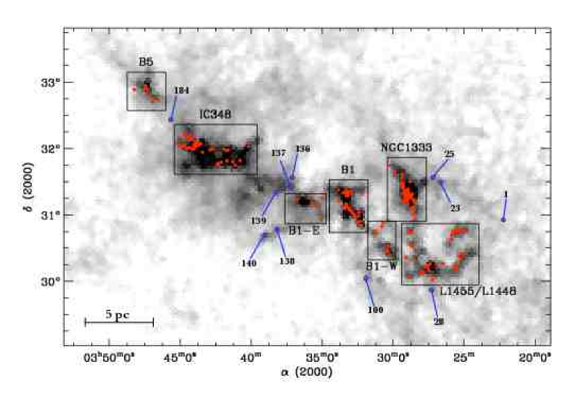
Figure 1.— Locations of GBT pointings (red points) overlaid upon a map of extinction for the Perseus region. Seven subregions have been defined and have their sources labeled in Figure 2. For sources outside the defined subregions, the sources are labeled on the map with the number of the source given in Table An Ammonia Spectral Atlas of Dense Cores in Perseus. The extinction map is derived from applying the NICER algorithm to 2MASS data (Ridge et al., 2006) and the grayscale has a square-root transfer function running from $A_{V}=0$ to 7 mag.

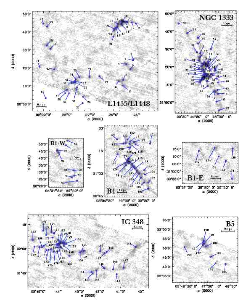
Figure 2.— Locations of GBT pointings (red points) overlaid upon a maps of millimeter emission from the BOLOCAM survey of the region (Enoch et al., 2006). The seven maps correspond to the subregions defined in Figure 1. Individual pointings are labeled with the number of the source given in Table An Ammonia Spectral Atlas of Dense Cores in Perseus. The grayscale has a square-root transfer function spanning $f_{\nu}=0$ to 400 mJy beam^-1.

The C${}_{2}^{34}$S line was not detected along any of the lines of sight. Given the ISM isotopic ratio ³²S/³⁴S $\sim 22$ (Wilson & Rood, 1994), the lack of any detections, particularly when the C₂S line is strong suggests that the main line is usually optically thin. For NH3SRC 42, we establish a lower limit on the line ratio of 11.7 (the maximum in our population) by setting the C${}_{2}^{34}$S amplitude to the 3$\sigma$ limit. Assuming excitation conditions are the same for both isotopomers, this implies $\tau_{\mathrm{CCS}}<1.4$ for one of the brightest C₂S lines in our sample.

In Figure 3 we show three spectra from our sample. Source 47 was observed every night as a consistency check on our flux calibration and is thus the best observed ammonia source in our sample (integrated S/N of 530). Source 89 shows a typical narrow line spectrum ($\sigma_{v}=0.12\mbox{ km s}^{-1}$) illustrating the resolution of the data. Source 31 is a multi-component spectrum which must be analyzed in more detail (see §3.4). In Source 31, the multiple components are also visible in the NH₃(2,2) and C₂S lines.

Figure 3.— Three sample spectra from the ammonia sample including the source used for a flux check (Source 47), a narrow-line spectrum (Source 89) and a multicomponent spectrum (Source 31).

We present a summary of our observations in Table An Ammonia Spectral Atlas of Dense Cores in Perseus. The properties of the cross-referenced names of the submillimeter cores are given in Enoch et al. (2006) and Kirk et al. (2006) respectively. Since ammonia has several hyperfine components that are well-separated in velocity, the integrated intensities reported for the (1,1) and the (2,2) lines are the sum of the integrated intensities over all channels that are within 3 km s^-1 of any hyperfine component. We subtract the mean intensity in the off-line channels between the hyperfine components from the intensity of each channel in the on-line windows to offset any low-lying baseline residuals. When there is no ammonia emission or C₂S from which the line velocity can be determined, the main component of the ammonia line is assumed to lie at the the mean ¹³CO velocity along the line of sight, as derived from the COMPLETE ¹³CO data.

3. Physical Parameter Estimation

Here we describe the estimation of physical parameters from the ammonia spectra. The method differs somewhat from previous work in that it forward models the properties of all observed spectral lines simultaneously given input physical properties. Then, the physical properties are derived using a non-linear least squares minimization code to determine the optimal fit to the observed spectrum. This stands in contrast with the standard method of obtaining these properties which relies on measuring line ratios and using these line ratios to calculate the physical properties. While the results should be the same using the two methods, the primary advantage of using a non-linear least squares fit is the automatic determination of uncertainties in the derived physical parameters as well as the covariances among those parameters (provided failures in the assumptions of the least-squares problem are appropriately accounted for). The model is optimized simultaneously for all observed spectra, which eliminates many systematic effects that arise from comparing properties derived from spectra separately. An additional advantage of this approach is that progressively more sophisticated models (e.g. De Vries & Myers, 2005) can be introduced to model specific spectral features. However, for this survey, we adopt a relatively simple model that can be applied to cores in a variety of environments.

For the spectra from a single object, a simple model is developed: the emission is assumed to arise from a homogeneous slab with uniform gas temperature, intrinsic velocity dispersion and uniform excitation conditions for all hyperfine transitions of the NH₃ lines. Detailed studies of NH₃ emission in conjunction with other molecular tracers illustrate the shortcomings of this model. The observations of Ladd et al. (1994) suggest that the ammonia emission is not completely uniform on $30^{\prime\prime}$ scales. Tafalla et al. (2004) note that the kinetic temperature of the two cores they study in detail is constant while there are radial variations in ammonia abundance and excitation temperatures in cores. Mauersberger et al. (1988) find the line width of the NH₃(2,2) transitions to be larger than the NH₃(1,1) transitions in the high-mass star forming region W3.

Despite these limitations, the uniform slab model is still useful. Lacking information about the spatial distribution of ammonia, a uniform slab is the simplest model we can adapt which should provide reasonable average properties over the region within the beam (see, for example, the conclusions of Tafalla et al., 2004). The GBT beam is roughly half the typical core radius for objects in Perseus Jijina et al. (1999, §2), so the emission should couple well to the GBT beam (hence our adoption of the main beam temperature scale). Separate fits to the line width of the strong NH₃ (1,1) and (2,2) detections show that the (2,2) line is, on average ($8\pm 2$)% wider than the (1,1) line. Several spectra show evidence for non-uniform excitation of ammonia hyperfine components. However, we emphasize that these deviations in excitation and line width are small (a few percent) and are only apparent because of the high quality of the data. In general, the slab model produces high-quality fits to the data. More complicated spectra (see Figure 4) merit further investigation and these interesting sources will be investigated in more detail elsewhere. This presentation of the data is restricted to generating average properties based on the simple model for comparison of physical properties across the sample.

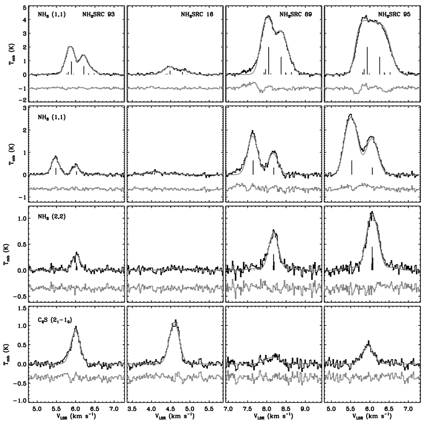
Figure 4.— Examples of fits to four GBT spectra. Each row shows a different excerpt from the spectra including (in order) the main component of the ammonia (1,1) complex, the satellite complex at $+19.85\mbox{ km s}^{-1}$ relative to the main complex (the $F_{1},F=0,1/2\to 1,1/2$ transition; the $F_{1},F=0,1/2\to 1,3/2$ transition is also visible, offset by $-0.54$ km s^-1), the main (2,2) complex and the C₂S line. The gray, smooth line shows the model spectrum and the residual is shown below each profile. Each column shows a different object including source 93, chosen for a good fit, source 16 chosen for a low optical depth fit, and sources 89 and 95 which show the slight deviations from the amplitude of the model in the case of high optical depth. The velocities and relative strengths of the NH₃ hyperfine structure are indicated with vertical lines.

3.1. Standard Spectral Model

Our GBT reduction pipeline produces three spectra with 1.846 kHz resolution centered on the NH₃ (1,1), NH₃ (2,2) and C₂S ($2_{1}\to 1_{0}$) transitions. The spectra are on the $T_{A}^{*}$ scale which include corrections for atmospheric opacity. We derive the physical parameters for a simple ammonia system: the gas is assumed to have a slab geometry with uniform properties, in particular gas kinetic temperature. The model assumes that column density of the material has a Gaussian distribution in velocity with a dispersion of $\sigma_{v}$ around an LSR velocity centroid $v_{LSR}$:

$$\frac{dN}{dv}dv=N_{0}\exp\left[-\frac{(v-v_{LSR})^{2}}{2\sigma^{2}_{v}}\right].$$ (1)

The ammonia (1,1) and (2,2) lines have 18 and 21 hyperfine components respectively so the optical depth implied by the column density distribution is split among each of the hyperfine components. As such, the opacity distribution for the (1,1) and (2,2) lines can be written (in terms of frequency on the sky with respect to the LSR) as:

$$\tau(\nu) = \tau_{1}\sum_{i=1}^{18}s_{i}\exp\left[-\frac{(\nu-\nu_{i}-\nu_{LSR})^{2}}{2\sigma_{i}^{2}}\right]$$ (2)

$$+ \tau_{2}\sum_{j=1}^{21}s_{j}\exp\left[-\frac{(\nu-\nu_{j}-\nu_{LSR})^{2}}{2\sigma_{j}^{2}}\right].$$

where $\nu_{LSR}$ is determined by the Doppler formula (radio convention):

$$\nu_{LSR}=\left(1-\frac{v_{LSR}}{c}\right)\nu_{rest}.$$ (3)

Above, $\tau_{1}$ ($\tau_{2}$) is the total opacity in the (1,1) [(2,2)] line transition; and $s_{i}$ ($s_{j}$) is statistical weight of the $i$th ($j$th) hyperfine component of the (1,1) [(2,2)] transition. Each component has a sky frequency $\nu_{i}$ ($\nu_{j}$) and a corresponding width $\sigma_{i}$ ($\sigma_{j}$) given by

$$\sigma_{i}=\frac{\sigma_{v}}{c}\nu_{i}$$ (4)

The number of molecules found in states that undergo the (1,1) vs. the (2,2) inversion transitions is governed by the rotation temperature of the system ($T_{R}$). Specifically, the population ratio is established by the magnitude of $T_{R}$ relative to the energy gap between the two states which (expressed in K) is $T_{0}=41.5$ K. The population ratio is given by the Boltzmann factor and the statistical weights of the two states [$g{(1,1)}$=3 and $g{(2,2)}=5$]. We assume that the transitions have equal line widths, $\sigma_{v}(1,1)=\sigma_{v}(2,2)$, and excitation temperatures, $T_{x}(1,1)=T_{x}(2,2)$. After including the amplitudes of the dipole matrix elements (e.g. $|\mu(1,1)|^{2}$), the ratio of the opacities can be expressed as (Ho et al., 1979; Ho & Townes, 1983):

$$\frac{\tau_{2}}{\tau_{1}} = \left[\frac{\nu_{(2,2)}}{\nu_{(1,1)}}\right]^{2}\frac{\sigma_{v}(1,1)}{\sigma_{v}(2,2)}\frac{T_{x}(1,1)}{T_{x}(2,2)}\frac{|\mu(2,2)|^{2}}{|\mu(1,1)|^{2}}\frac{g{(2,2)}}{g{(1,1)}}\exp\left(-\frac{T_{0}}{T_{R}}\right)$$ (5)

$$= \left[\frac{\nu_{(2,2)}}{\nu_{(1,1)}}\right]^{2}\frac{20}{9}\exp(-T_{0}/T_{R}).$$ (6)

We assume that the kinetic temperature $(T_{k})$ is much less than $T_{0}$, implying that the (1,1) and (2,2) states are the only populated rotational levels of the ammonia system. Thus, it is a two-state system for which the kinetic temperature can be related to the rotation temperature with knowledge of the collision coefficients using detailed balance arguments (Swift et al., 2005). In this case:

$$T_{R}=T_{k}\left\{1+\frac{T_{k}}{T_{0}}\ln\left[1+0.6\exp\left(-15.7/T_{k}\right)\right]\right\}^{-1}.$$ (7)

Finally, given a radiation excitation temperature, $T_{x}$, the two ammonia spectra can now be modeled in their entirety:

$$T_{A}^{*}(\nu)=\eta_{mb}(\nu)\eta_{f}\left[J(T_{x})-J(T_{bg})\right]\left[1-e^{-\tau(\nu)}\right]$$ (8)

where $\eta_{mb}(\nu)$ is the main beam efficiency of the GBT ($\approx 0.81$ for the frequency range in this study), $\eta_{f}$ is the filling fraction of the emission in the beam, $T_{bg}=2.73$ K and

$$J(T)=\frac{h\nu}{k}\frac{1}{\exp(h\nu/kT)-1}.$$ (9)

After making assumptions about source-beam coupling and filling fraction, the spectrum is entirely determined by five parameters: $T_{k},T_{x},\tau_{1},\sigma_{v},$ and $v_{LSR}$. Alternatively, we can assume that $T_{x}=T_{k}$ (LTE) and let the filling fraction $\eta_{f}$ vary.

In addition to the ammonia system, we also measure spectra for the C₂S line. We also fit a three parameter Gaussian to the C₂S line simultaneously while deriving parameters for the ammonia spectra. The total spectral model is given by:

$$T_{A}^{*}(\mbox{model})=T_{A}^{*}(\mbox{NH}_{3})+\eta_{mb}(\nu)T_{\mathrm{CCS}}\exp\left[-\frac{(\nu-\nu_{0}-\nu_{LSR}-\nu_{off})^{2}}{2\sigma_{\mathrm{CCS}}^{2}}\right]$$ (10)

Here, $\nu_{0}$ is the given rest frequency of the C₂S line, $\nu_{LSR}$ is the appropriate frequency shift account for motion with respect to the LSR using the same LSR velocity as derived from NH₃. We define a velocity offset $V_{off}$ which, via the Doppler formula, relates to the derived frequency offset $\nu_{off}$. $T_{\mathrm{CCS}}$ and $\sigma_{\mathrm{CCS}}$ are the amplitude and derived width of the line. We do not know the excitation temperature of the C₂S line, but we assume the excitation is similar to that of ammonia since the critical density ($n_{cr}\sim 10^{4.5}\mbox{cm}^{-3}$, Langer et al., 1995) is close to that of the ammonia lines (Swade, 1989). The C₂S line complex adds the parameters $T_{\mathrm{CCS}}$, $\sigma_{\mathrm{CCS}}$ and $V_{off}$ to our fit.

The final effect we account for is the sampling of the GBT correlation spectrometer. The lags in the spectrometer are weighted uniformly (i.e. no online smoothing). As a result, a channel has a nominal profile of a sinc function:

$$\phi(\nu)=\frac{\sin\left[\pi\left(\nu-\nu_{k}\right)/\Delta\nu\right]}{\pi\left(\nu-\nu_{k}\right)/\Delta\nu}.$$ (11)

Here, $\nu_{k}$ is the channel center and $\Delta\nu$ is the channel spacing. After deriving $T_{A}^{*}(\mbox{model})$, we digitally sample it at one-fourth the channel spacing and we convolve the model spectrum with channel profile to produce the final result which is compared with observations.

We find the maximum likelihood model for the spectrum using a non-linear least-squares fitting routine. The optimization occurs in two steps: first the fit is performed to the entirety of the NH₃(1,1), NH₃(2,2) and C₂S spectra. If emission is detected the fit is performed again, ignoring regions of the spectrum more than 2.5 km s^-1 away from significant emission using the results of the first fit as an initial guess for the optimization. This second step reduces the number of noise-only channels in the fit and allows for a cleaner convergence to an optimal set of properties. Examples of the fitting appear in Figure 4. We have chosen four representative spectra for several cases found in the single-component models. The first two columns of the figure show the successful applications of the model in the regular and low optical depth regimes (§3.2). The final two columns of the figure show the slight deviations frequently encountered in spectra with high optical depth in the lines. The slight deviations may be the result of non-LTE excitation of the different hyperfine components. Several other spectra show asymmetries in the line profiles for which a Gaussian model of the velocity distribution is inaccurate (see §3.4 for further discussion of these cases). The full set of spectra for lines of sight with detections are available as online-only figures (Figure 7a–6ff) and are downloadable from the COMPLETE website.

3.2. Low Optical Depth Regime

When $\tau(\nu)\ll 1$ for the ammonia complex over all $\nu$, the parameters $T_{x}$ and $\tau_{11}$ become degenerate and it is impossible to solve for the two parameters independently. In this case, we expand Equation 8 assuming the Rayleigh-Jeans limit so that

$$T_{A}^{*}(\nu)=\eta_{mb}(\nu)\eta_{f}\left(T_{x}-T_{bg}\right)\tau(\nu)$$ (12)

where $\tau(\nu)$ is given by Equation 2. In this case, we optimize the fit for the free parameter $\gamma\equiv\left(T_{x}-T_{bg}\right)\tau_{1}$ and the ammonia spectrum is determined by four free parameters: $T_{k},\gamma,\sigma_{v}$, and $v_{LSR}$. This approximation is accurate to better than 10% for all components of the ammonia complex provided $\tau_{1}<1$.

3.3. Column Density Estimates

We measure the total column density of NH₃ and C₂S using the derived parameters from the fit. For example, the column density in the NH₃ (1,1) state is (e.g. Rohlfs & Wilson, 2004):

$$N(1,1)=\frac{8\pi\nu_{0}^{2}}{c^{2}}\frac{g_{1}}{g_{2}}\frac{1}{A_{(1,1)}}\left[1-\exp\left(\frac{h\nu_{0}}{kT_{x}}\right)\right]^{-1}\int\tau(\nu)d\nu$$ (13)

The statistical weights of the upper and lower levels of the inversion transition are equal. The Einstein A value for the inversion transition is $A_{(1,1)}=1.68\times 10^{-7}\mbox{ s}^{-1}$ (Pickett et al., 1998). The opacity per unit frequency is given in terms of the total opacity of the line ($\tau_{1}$) by the first term in Equation 2.

$$\int\tau(\nu)d\nu = \tau_{1}\int d\nu\sum_{i}s_{i}\exp\left[-\frac{(\nu-\nu_{i}-\nu_{LSR})^{2}}{2\sigma_{i}^{2}}\right]$$ (14)

$$= \sqrt{2\pi}\sigma_{i}\tau_{1}=\sqrt{2\pi}\frac{\sigma_{v}}{c}\nu_{0}\tau_{1}$$

under the approximation that the frequencies of the individual hyperfine components are the same ($\nu_{0}$). The partition function for the metastable states ($J=K$) of ammonia is given by (Rohlfs & Wilson, 2004):

$$Z=\sum_{J}(2J+1)~{}S(J)~{}\exp\left\{\frac{-h[B~{}J(J+1)-(C-B)J^{2}]}{kT_{K}}\right\}$$ (15)

Here, $B$ and $C$ are the rotational constants of the ammonia molecule: 298117 MHz and 186726 MHz respectively (Pickett et al., 1998). The factor $S(J)$ equals 2 for $J=3,6,9\dots$ and 1 otherwise, accounting for the extra statistical weight of ortho-NH₃ over para-NH₃. Owing to the relatively short lifetime of the $J\neq K$ states, we assume all ammonia molecules are in the metastable states. To determine the total column density, we scale the column density in the (1,1) state by $Z/Z(J=1)$. We truncate the partition function at 50 terms.

For the low optical depth case, we expand the exponential in Equation 13:

$$N(1,1) = \frac{8\pi k\nu_{0}}{hc^{2}}\frac{1}{A_{(1,1)}}\int T_{x}\tau(\nu)d\nu$$ (16)

$$= \frac{8\pi k\nu_{0}^{2}}{hc^{3}}\frac{1}{A_{(1,1)}}\sqrt{2\pi}\sigma_{v}~{}(T_{x}-T_{bg})\tau_{1}$$

where $\sigma_{v}$ and $(T_{x}-T_{bg})\tau_{1}$ are determined by the low-optical-depth fit (§3.2).

We also estimate the column density of C₂S assuming that the line is optically thin, an assumption bolstered by our failure to detect C₂³⁴S along any of the lines-of-sight.

$$N(\mathrm{C_{2}S},J=1)=\frac{8\pi k\nu_{0}}{hc^{2}}\frac{g_{1}}{g_{2}}\frac{1}{A_{21}}\sqrt{2\pi}\sigma_{v}~{}(T_{x}-T_{bg})\tau_{21}.$$ (17)

Here, $g_{J}=2J+1$, $A_{21}=5.44\times 10^{-7}\mbox{ s}^{-1}$ (Pickett et al., 1998) and we take $(T_{x}-T_{bg})\tau_{21}=T_{\mathrm{CCS}}$. Again, we calculate the total column density of C₂S using the partition function. For a state with energy above the ground state $E_{i}$ and degeneracy $g_{i}$, the partition function is the standard

$$Z=\sum_{i}g_{i}\exp\left[-\frac{E_{i}}{kT_{k}}\right].$$ (18)

We adopt the values of $E_{i}$ and $g_{i}$ from the tabulated molecular data in the JPL molecular spectroscopy catalog (Pickett et al., 1998) and assume the 295 states are thermally populated. It may not be appropriate to use the kinetic temperature derived from the NH₃ for the C₂S partition function since the two species may not be thermally coupled. This systematic effect limits our ability to measure the C₂S column. For both molecules, the uncertainties in the column density are established by adding a normal deviate times the uncertainty to the input parameters and recalculating the column densities. After repeating this redistribution within the errors a large number of times, the error are determined from the width of the resulting distribution.

We tested the results of the uniform slab modeling by comparing the results to the values derived from the hyperfine fitting routines in the CLASS package. We checked the line width, opacity, excitation temperature and LSR velocity. The results were identical within the errors of our analysis except for complex source spectra (e.g. asymmetric profiles, multiple components).

3.4. Multi-Component Fitting

Several of the spectra show significant velocity structure in the line beyond what is expected from the hyperfine structure of ammonia (see, for example, Source 31 in Figure 3). In cases where the number of components is readily modeled, we have attempted to fit a multicomponent model to the spectrum. In this model, we assume that there are two objects in the beam each with $\eta_{f}<1$ and we operate in the LTE approximation ($T_{x}=T_{k}$). Hence, it is not necessary to calculate radiative transfer effects of one component through another. The approximation appears to be sufficiently good for our purposes.

We only present multiple components to the data where the evidence is unambiguous that a multiple-component fit is appropriate. This means two clear peaks in the NH₃ (2,2) line. In some cases the velocity separation is sufficient that multiple components are also well distinguished in the (1,1) line. The initial conditions for the fit are established by hand, but the optimization is performed simultaneously for both components. To prevent run-away solutions, we constrain the initial velocities to be within 0.1 km s^-1 of the initial guess and also constrain the C₂S and NH₃ velocities to be within 0.1 km s^-1 for each of the components. We report the fits to the multiple components independently in Table An Ammonia Spectral Atlas of Dense Cores in Perseus appending a decimal and the number of the component onto source name. In the six spectra with multiple components reported, all show that the sum of the their filling fractions is less than unity. The typical filling fraction for a single component is $\eta_{f}=0.3$.

Seven additional spectra show strong evidence for multiple components in some or all of the lines. In particular, there are often multiple components in the C₂S and a broad or poorly fit NH₃ (1,1) line but no clear evidence for multiple components in the NH₃ (2,2) line. Since we cannot be certain that these two components in C₂S are physically associated with two components in NH₃, we refrain from performing a multicomponent fit but note the presence of the components in Table An Ammonia Spectral Atlas of Dense Cores in Perseus. There are a number of additional spectra with weaker evidence of multiple components, or evidence for more than two components. We likewise flag these objects in Table An Ammonia Spectral Atlas of Dense Cores in Perseus.

3.5. Uncertainties and Limits in Derived Parameters

The reported uncertainties in Table An Ammonia Spectral Atlas of Dense Cores in Perseus are the derived uncertainties from the nonlinear least-squares fitting using the covariance matrix. The individual channels are not independent (the channel width is 1.525 kHz and the resolution is 1.862 kHz) which violates an assumption of least-squares fitting. The errors determined reported from the covariance matrix represent the $\Delta\chi^{2}=1$ ellipsoid. To determine appropriate uncertainties, we generated multiple realizations of several different spectral models each with different noise distributions. We used our fitting routine to derive parameters in the presence of noise and compared the distribution of the derived parameters to the input model parameters. Over all the different spectral models, the true errors were a factor of $\leq 1.6$ larger than the errors derived from the covariance matrix assuming the data were independent. While not technically a least-squares fit, accurate confidence intervals for the derived parameters can still be estimated using the $\Delta\chi^{2}=2.56=1.6^{2}$ surface (Press et al., 1992). We have investigated the shape of $\chi^{2}$ space in our data and find that the region around the minimum $\chi^{2}$ is well approximated by a paraboloid. To report errors consistent with a $1\sigma$ spread around the derived parameters, we scale the reported errors up by a factor of 1.6.

The covariance matrix also indicates which parameters are correlated with each other in the fits. The additional uncertainty due to this correlation is accounted for in the reported errors. For parameters $i$ and $j$, we express the covariance in terms of the normalized covariance: $\sigma_{ij}/(\sigma_{i}\sigma_{j})^{1/2}$. We examined the average covariance matrix over the 133 fits with sufficiently strong NH₃(1,1) emission to fit for optical depth and excitation temperature separately. We find that the most obvious (anti)correlation is between $T_{ex}$ and $\tau$: $\sigma_{ij}/(\sigma_{i}\sigma_{j})^{1/2}=-0.95$. This strong anticorrelation necessitates the low opacity treatment described in §3.2. The excitation temperature is also correlated with $T_{K}$ (0.18) and $\sigma_{v}$ (0.24). The line opacity ($\tau_{i}$) has an anticorrelation with the line width $\sigma_{v}$ ($-0.49$) and $T_{k}$ ($-0.23$). For the C₂S line, there is the anticorrelation between the amplitude ($T_{\mathrm{CCS}}$) and the line width $\sigma_{\mathrm{CCS}}$ typical of Gaussian fits ($-0.57$ in our case). The other elements of the covariance matrix are consistent with zero.

The uncertainties do not reflect the overall uncertainty in the amplitude scale calibration which is $\sim 5\%$, The relative calibration across the spectra is much better than $5\%$, so certain properties are unaffected by the overall amplitude calibration. The integrated intensities reported in Table An Ammonia Spectral Atlas of Dense Cores in Perseus as well as properties derived from the amplitude of the emission (column densities, excitation temperatures, filling fractions, and antenna temperatures) have $\sim 5\%$ uncertainties. In contrast, line-of-sight velocities, line widths, optical depths and kinetic temperatures (since the latter two are driven by line ratios) have uncertainties close to their reported precisions.

In several cases, we detect the (1,1) transition of NH₃ but not the (2,2) transition. When we can establish an upper limit on the intensity of (2,2) line, we report a $3\sigma$ upper limit on the temperature of the ammonia. Since the ammonia temperature is used in the calculation of column densities, the upper limit on temperature produces a lower limit on the NH₃ column density since the partition function correction is a decreasing function of temperature for $T_{k}<40$ K. In contrast, the correction for C₂S is an increasing function of temperature so the upper limit of temperature creates an upper limit for the C₂S column density.

The velocity width of the ammonia complex is quoted as an upper limit in Table An Ammonia Spectral Atlas of Dense Cores in Perseus for instances when (1) there are multiple components along the line of sight that cannot be decoupled and fit separately or (2) when the line widths are large but the signal-to-noise is small such that the broadening of the line cannot be distinguished from the splitting due to the hyperfine structure. In the latter case, the upper limit reported may represent the actual value, but we cannot distinguish between a large intrinsic line width and line widths that result from the hyperfine structure. We note that we find no cores with large ammonia (1,1) antenna temperatures ($T_{A}^{*}>1\mbox{ K}$), large line widths ($\sigma_{v}>0.2\mbox{ km s}^{-1}$) which have no evidence for multiple components along the line of sight. Said differently, all large line width cores may have large line widths only because of multiple components along the line of sight.

The largest systematic in the reported values is the bias introduced by the uniform slab model presented above. Again, we emphasize that the model is adopted for uniform application to a large sample; individual spectra can be investigated in more detail. One difficulty in applying our model may occur in comparing the (1,1) and (2,2) emission. Although the critical densities for the two transitions are similar, the NH₃(1,1) emission has larger optical depths than the (2,2) emission. In cores with radial gradients in temperature, opacity effects may result in the (2,2) emission revealing warmer gas than the (1,1) emission. We have attempted fitting the most optically thick spectra with the hill models of De Vries & Myers (2005), but we do not find a significant improvement in the fit quality with the additional complications the model entails. Such line-of-sight variations in the excitation conditions are ignored in our simple treatment, but our derived values should yield (appropriately weighted) average conditions along the line of sight.

3.6. Comparison to Previous Work

Ammonia has been observed towards Perseus in several previous studies. We compare the derived properties from our analysis to those values found in the literature for sources other studies have observed. For comparison, we use homogenized properties in the catalog of Jijina et al. (1999) which are drawn primarily from the work of Ladd et al. (1994); Bachiller & Cernicharo (1986); Bachiller et al. (1987) and Juan et al. (1993). We find good agreement between our line widths and temperatures with $\lesssim 20\%$ variations across most of our sources. Discrepant points are invariably found in NGC 1333 where larger line widths are typically found in earlier studies. We suspect that the larger beam sizes of previous work blend together more disparate emission than the GBT observations resulting in the larger line widths. The agreement with ammonia column density is less well established with variations up to 0.5 dex are found. However, the largest discrepancies are associated with highly uncertain column densities flagged in Jijina et al. (1999). We conclude that these new data match the results of previous studies quite well with significant variations attributable to the improved quality of the observations.

4. Distributions of Derived Properties

In this section, we present a brief summary of the observed spectra and their derived properties. A graphical summary of the data that appear in Tables An Ammonia Spectral Atlas of Dense Cores in Perseus and An Ammonia Spectral Atlas of Dense Cores in Perseus is given in Figure 5. The first two panels show the typical distribution of line temperatures on the $T_{mb}$ scale for the (sub)millimeter (gray) and all other sources. The strongest sources are all associated with millimeter-bright objects and other targets are typically weak in (1,1) emission and infrequently detected in (2,2). Two sources, NH3SRC 27 and 60, are outside the bounds of either (sub)millimeter study but we detect significant line emission. We have included these in the millimeter-faint population since they are only associated with MIPS-derived dust features, but this assignment may be incorrect.

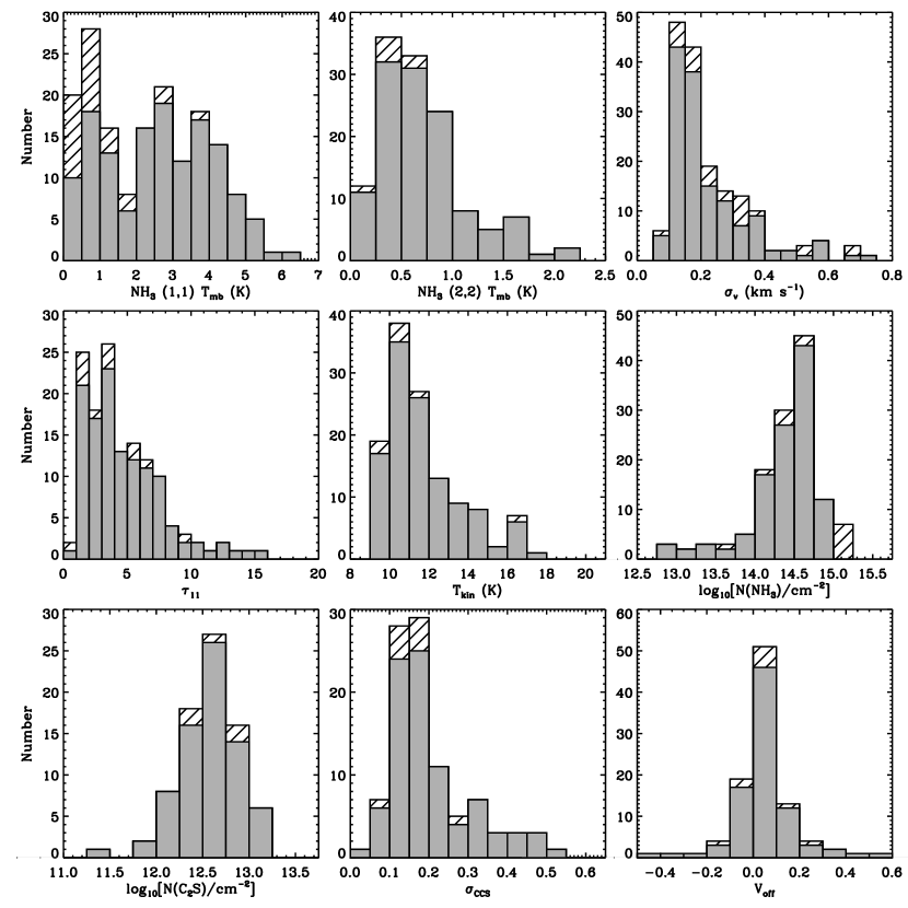
Figure 5.— Distribution of the observed and derived properties for the GBT spectra. Working from left to right, top to bottom, the nine panels show the peak main beam temperatures for the (1,1) and (2,2) lines, the intrinsic velocity dispersion of NH₃ derived from the (1,1) and (2,2) lines (including upper limits as data), the total optical depth of the (1,1) complex, the kinetic temperature of the gas, the column density of the ammonia emission, the column density of the C₂S, the velocity dispersion of the C₂S line, and the velocity offset of the C₂S line from the ammonia complex. The gray histogram shows the distributions of properties for the pointings associated with (sub)millimeter sources and the hashed histogram shows all remaining objects. Objects are included in the histograms only if they have well-determined values for the properties reported (with the exception of line width).

The derived intrinsic line widths are typically $<0.2$ km s^-1 across the entire sample with a high line width tail to the distribution. As noted previously, these line widths may be upper limits since in all cases where there is sufficient signal-to-noise to resolve the structure of the line there is evidence for multiple velocity components. The typical (total) optical depth of the ammonia complex is $\sim 4$ and the main complex has a thickness half the optical depth shown. Hence, in most cases, the lines are only moderately opaque, though some line complexes are quite optically thick. The (sub)millimeter-weak sources have a higher median line width and lower opacity than the (sub)millimeter-bright population.

The derived kinetic temperatures of the cores are uniformly cool (T${}_{K}<20$ K) and are typically 11 K, substantially lower than is assumed in some work (e.g. Kirk et al., 2006) for submillimeter cores. If the dust and gas are well-coupled, assuming $T=15$ K for the Perseus cores can result in underestimating the mass of the cores by a factor of 1.7. However, assuming a temperature of 10 K yields a typical overestimate by a factor of 1.2. To accurately determine the masses of cores from the millimeter continuum requires temperature determinations for every core. After this correction, the dominant contribution to the uncertainties in the core masses is the dust opacity at these wavelengths.

The column density of ammonia is typical for cores in Perseus (Jijina et al., 1999). However, the sensitive observations also find some spectra that imply $N(\mbox{NH}_{3})<10^{13.5}\mbox{ cm}^{-2}$, making these detections among the lowest column densities of ammonia yet found. The low column density detections are all associated with the IC348 region of the cloud. The C₂S column densities also appear typical of dense cores (Suzuki et al., 1992) but are subject to uncertainty based on unknown temperatures and excitation conditions.

The velocity dispersions of the C₂S lines are comparable to those of the ammonia lines, and the C₂S lines show a slight, systematic offset in velocity from the ammonia complex. This offset is likely due to uncertainties in the assumed rest frequency of the C₂S line. The mean offset is 16 m s^-1 (weighting by the inverse variance of the measurements) and would be consistent with zero for a rest frequency of $\nu_{\mathrm{CCS}}=22.344032(1)$ GHz. The difference is within the uncertainties of the assumed frequency.

We conclude this section by noting several spectra that define the extent of the property distributions or are otherwise notable. Plots of the spectra are available in the online-only edition (Figure 7a–6ff).

Typical Spectrum – NH3SRC 15 is the “most typical” ammonia spectrum from Perseus with nearly average values of all the properties shown in Figure 5. For NH3SRC 15, $T_{kin}=11.2$ K, $\sigma_{v}=0.19$ km s^-1, $\tau_{1,1}=3.7$, and $N(\mbox{NH}_{3})=3.1\times 10^{14}\mbox{ cm}^{-2}$.

Temperature Range – NH3SRC 18 has the lowest, well-determined temperature of the observed sources ($T_{kin}=9.05$ K) and NH3SRC 116 has the highest temperature ($T_{kin}=26$ K).

Column Density – NH3SRC 144 has the lowest column density detected in our survey ($5.5\times 10^{12}$ cm^-2) and NH3SRC 17 has the highest column density ($1.3\times 10^{15}$ cm^-2).

Line Brightness – NH3SRC 54 is the faintest source in NH₃(1,1) emission included as a detection ($W_{mb}=0.2$ K km s^-1) and NH3SRC 12 is the strongest (20.0 K km s^-1). In the (2,2) line, NH3SRC 19 is the weakest ($W_{mb}=0.03$ K km s^-1) and NH3SRC 68 is the strongest ($W_{mb}=2.27$ K km s^-1). In the C₂S line, NH3SRC 21 is the weakest detection ($W_{mb}=0.07$ K km s^-1) while NH3SRC 42 is the strongest ($W_{mb}=0.67$ K km s^-1).

Line Width – The narrowest line width source we detect is NH3SRC 128 with a line width of 0.079 km s^-1. The largest line width we reliably detect is 0.23 km s^-1 in NH3SRC 109. However, many of the fits yield larger results such as NH3SRC 71 where the measured line width is 0.72 km s^-1 though the fit is unreliable. In addition many spectra show odd structure in their line profiles including wings (NH3SRCs 70, 127) and plateaus (NH3SRC 75) in addition to the multicomponent structure discussed previously (§3.4).

5. Summary

We have searched for NH₃(1,1), NH₃(1,1), C₂S($2_{1}\to 1_{0}$) emission along 193 lines of sight towards the Perseus molecular cloud. The lines of sight were selected based on positions that were detected in (sub)millimeter emission or had large dust column densities implied by far infrared (FIR) emission. We detect ammonia emission along 162 (84%) of the lines of sight and C₂S along 96 (51%) of the lines of sight. We estimate the physical properties of the gas by fitting a model emission profile to all spectral lines simultaneously. The emission is modeled as a uniform slab of gas that completely fills the beam, has a Gaussian intrinsic line width, and a single excitation temperature for all lines. Where appropriate, we refined the model to account for low optical depths, incomplete coupling to the GBT beam and multiple velocity components along the line of sight.

Nearly all (98%) bright, (sub)millimeter cores have strong ammonia emission associated with them and the exceptions appear to be artifacts in the submillimeter map based on examining the original BOLOCAM data. In addition, we detected emission towards 23 sources selected based on FIR emission that implies large dust column densities and low temperatures. Twenty-one objects are not seen in the (sub)millimeter, suggesting that the submillimeter emission is not a perfect tracer of the dense gas (the remaining two sources are outside the bounds of the continuum surveys). However, the FIR-based ammonia detections have lower line intensities than (sub)millimeter-bright source, as well as lower optical depths and larger line widths. It remains to be shown whether this could be an evolutionary effect or whether the (sub)millimeter-weak sources simply trace isolated pockets of gas not associated with the dense cores traced by the dust continuum.

We find that the ammonia implies dense gas temperatures in Perseus are predominantly cold ($T_{k}\sim 11~{}$K). Ammonia column densities are typical for cores presented in the literature ($N_{\mathrm{NH3}}\sim 10^{14.5}\mbox{ cm}^{-2}$, Jijina et al., 1999) though we also find several lines-of-sight with very low ammonia column densities ($N_{\mathrm{NH3}}\lesssim 10^{13.5}\mbox{ cm}^{-2}$) associated with the IC 348 region.

Forthcoming work will examine the properties of these objects in more detail including comparison with the (sub)millimeter emission, protostellar content, and the velocity structure of the dense core population.

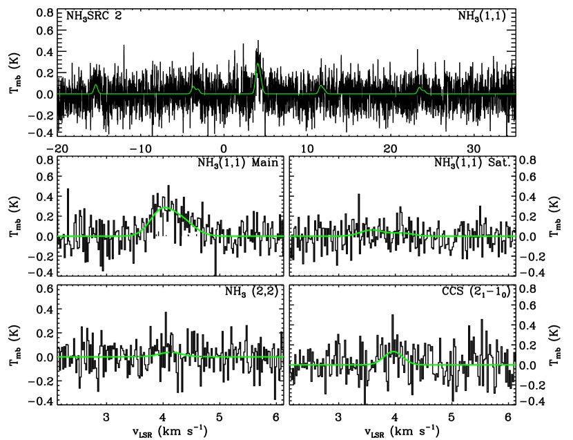
Figure 7a.— (top) The full NH₃(1,1) spectrum of NH₃SRC 1. The spectrum is shown in black, the best fitting model described in §3 is shown in green. Where discernible, additional velocity components are plotted in blue. (middle,left) The central component of the NH₃(1,1) line and best fitting model. The velocities and relative amplitudes of the hyperfine components are indicated with vertical lines. (middle, right) The NH₃(1,1) high-velocity hyperfine satellite at $\Delta v=19.85\mbox{ km s}^{-1}$ and best fitting model. Hyperfine components are indicated with vertical lines. (bottom, left) The main component of NH₃(2,2) line and best fitting model. Hyperfine components are indicated with vertical lines. (bottom, right) The C₂S ($2_{1}\to 1_{0}$) line and best fitting model.

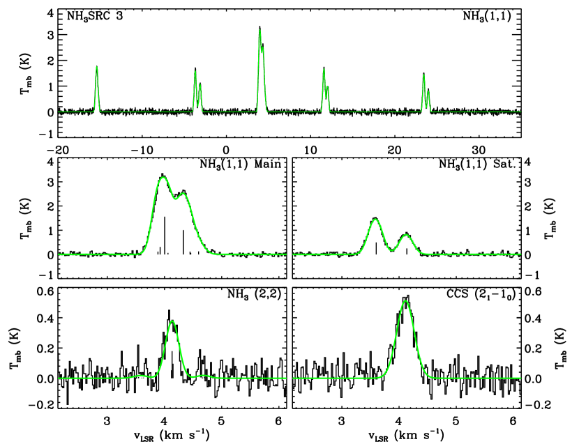
Figure 8b.— As Figure 8a but for NH₃SRC 3.

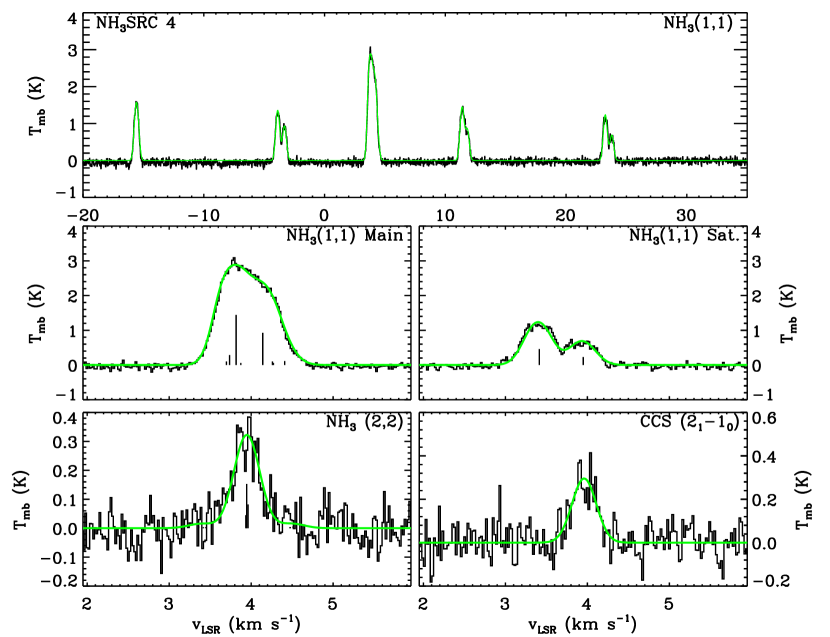
Figure 9c.— As Figure 9a but for NH₃SRC 4.

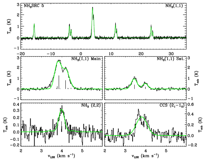
Figure 10d.— As Figure 10a but for NH₃SRC 5.

Table 2Summary of Observations

NH3SRC	Origin	Region	Position	Bolocam	SCUBA	Int. Time	$\sigma_{rms}$	$W[\mathrm{NH}_{3}(1,1)]$	$W[\mathrm{NH}_{3}(2,2)]$	$W[\mathrm{C_{2}S}]$
			($\alpha_{2000}$, $\delta_{2000}$)	Name	Name	(min.)	(mK)	(K km s-1)	(K km s-1)	(K km s-1)
(1)	(2)	(3)	(4)	(5)	(6)	(7)	(8)	(9)	(10)	(11)
1	D	$\cdots$	03:22:18.9 +30:53:14	$\cdots$	N/A	5	120	0.07(8)	0.03(3)	0.00(4)
2	D	L1455/L1448	03:25:00.3 +30:44:10	$\cdots$	$\cdots$	5	128	0.46(9)	0.02(4)	0.05(5)
3	B	L1455/L1448	03:25:07.8 +30:24:22	1	$\cdots$	15	63	5.25(4)	0.15(2)	0.22(2)
4	B	L1455/L1448	03:25:09.7 +30:23:53	2	$\cdots$	15	60	5.87(4)	0.12(2)	0.09(2)
5	B	L1455/L1448	03:25:10.1 +30:44:41	3	$\cdots$	15	63	4.08(4)	0.10(2)	0.23(2)
6	B	L1455/L1448	03:25:17.1 +30:18:53	4	N/A	20	54	2.21(4)	0.04(1)	0.36(2)
7	B	L1455/L1448	03:25:22.3 +30:45:09	5	032537+30451	15	60	10.09(4)	0.67(2)	0.20(2)
8	S	L1455/L1448	03:25:26.2 +30:45:05	$\cdots$	032543+30450	10	87	12.36(6)	0.79(2)	0.34(3)
9	B	L1455/L1448	03:25:26.9 +30:21:53	6	N/A	15	61	4.43(4)	0.10(2)	0.23(2)
10	D	L1455/L1448	03:25:32.3 +30:46:00	$\cdots$	$\cdots$	10	74	2.93(5)	0.10(2)	0.06(3)
11	B	L1455/L1448	03:25:35.5 +30:13:06	7	N/A	15	58	0.94(4)	0.04(2)	0.36(2)
12	B	L1455/L1448	03:25:36.2 +30:45:11	8	032560+30453	20	54	19.97(4)	1.65(1)	0.24(2)
13	B	L1455/L1448	03:25:37.2 +30:09:55	9	N/A	20	44	0.61(3)	0.04(1)	0.12(2)
14	B	L1455/L1448	03:25:38.6 +30:43:59	10	032564+30440	10	62	13.29(4)	1.29(2)	0.38(2)
15	B	L1455/L1448	03:25:46.1 +30:44:11	11	$\cdots$	10	61	5.62(4)	0.26(2)	0.16(2)
16	B	L1455/L1448	03:25:47.5 +30:12:26	12	N/A	20	41	0.71(3)	0.02(1)	0.36(2)
17	B	L1455/L1448	03:25:48.8 +30:42:24	13	032581+30423	15	40	11.49(3)	0.34(1)	0.26(2)
18	B	L1455/L1448	03:25:50.6 +30:42:02	14	$\cdots$	10	66	10.32(5)	0.27(2)	0.25(3)
19	B	L1455/L1448	03:25:55.1 +30:41:26	15	$\cdots$	25	42	1.63(3)	0.03(1)	0.20(2)
20	B	L1455/L1448	03:25:56.4 +30:40:43	16	$\cdots$	25	39	0.80(3)	0.02(1)	0.16(1)
21	B	L1455/L1448	03:25:58.5 +30:37:14	17	$\cdots$	25	39	0.89(3)	0.02(1)	0.07(2)
22	B	L1455/L1448	03:26:37.0 +30:15:23	18	032662+30153	10	60	4.89(4)	0.30(2)	0.26(2)
23	D	$\cdots$	03:26:39.7 +31:28:21	N/A	N/A	5	94	0.30(7)	0.02(3)	0.07(4)
24	B	L1455/L1448	03:27:02.1 +30:15:08	19	$\cdots$	15	44	1.74(3)	0.05(1)	0.21(2)
25	D	$\cdots$	03:27:14.3 +31:32:49	$\cdots$	N/A	5	138	0.7(1)	0.06(4)	-0.04(5)
26	D	L1455/L1448	03:27:20.2 +30:04:26	$\cdots$	N/A	10	77	0.95(5)	0.04(2)	0.00(3)
27	D	L1455/L1448	03:27:20.5 +30:00:42	N/A	N/A	5	108	0.75(7)	0.08(3)	0.18(4)
28	D	$\cdots$	03:27:26.4 +29:51:08	N/A	N/A	10	122	0.74(8)	0.01(4)	0.19(5)
29	B	L1455/L1448	03:27:28.9 +30:15:04	20	$\cdots$	20	54	4.51(4)	0.16(2)	0.36(2)
30	L	L1455/L1448	03:27:34.4 +30:09:22	$\cdots$	$\cdots$	5	87	1.54(6)	0.02(2)	0.13(3)
31	B	L1455/L1448	03:27:37.7 +30:14:00	21	032763+30139	30	38	6.04(3)	0.31(1)	0.15(1)
32	B	L1455/L1448	03:27:39.3 +30:12:59	22	032765+30130	20	45	10.56(3)	0.85(1)	0.20(2)
33	S	L1455/L1448	03:27:40.0 +30:12:13	$\cdots$	032766+30122	5	136	11.96(9)	0.55(4)	0.30(6)
34	B	L1455/L1448	03:27:41.9 +30:12:30	23	032771+30125	20	41	10.78(3)	0.61(1)	0.25(2)
35	B	L1455/L1448	03:27:47.9 +30:12:02	24	032780+30121	30	39	6.36(3)	0.38(1)	0.16(2)
36	L	L1455/L1448	03:27:55.9 +30:06:18	$\cdots$	N/A	5	84	4.96(6)	0.12(2)	0.17(3)
37	L	L1455/L1448	03:28:00.7 +30:08:20	$\cdots$	$\cdots$	5	132	4.01(9)	0.18(4)	0.25(5)
38	L	L1455/L1448	03:28:05.5 +30:06:19	$\cdots$	N/A	5	80	5.00(6)	0.14(2)	0.14(3)
39	W	NGC1333	03:28:30.0 +30:55:29	$\cdots$	$\cdots$	5	131	0.09(9)	-0.01(4)	0.05(6)
40	B	NGC1333	03:28:32.2 +31:11:09	25	$\cdots$	15	38	5.36(3)	0.25(1)	0.05(2)
41	B	NGC1333	03:28:32.4 +31:04:43	26	$\cdots$	10	54	6.36(4)	0.29(2)	0.10(2)
42	B	L1455/L1448	03:28:33.4 +30:19:35	27	$\cdots$	15	68	2.24(5)	0.12(2)	0.66(2)
43	B	NGC1333	03:28:34.1 +31:07:01	28	$\cdots$	15	54	3.01(4)	0.12(2)	0.06(2)
44	B	NGC1333	03:28:36.3 +31:13:27	29	032861+31134	15	41	5.26(3)	0.34(1)	0.02(2)
45	W	NGC1333	03:28:36.8 +31:00:14	$\cdots$	$\cdots$	5	142	0.00(1)	0.00(4)	0.03(6)
46	B	NGC1333	03:28:39.1 +31:06:00	30	032865+31060	10	57	8.85(4)	0.42(2)	0.24(2)
47	S	NGC1333	03:28:39.5 +31:18:35	$\cdots$	032865+31185	41	34	12.60(2)	0.847(9)	0.18(1)
48	S	NGC1333	03:28:40.3 +31:17:56	31	032866+31179	5	170	16.2(1)	1.09(4)	0.10(7)
49	B	L1455/L1448	03:28:41.7 +30:31:12	32	$\cdots$	15	41	0.94(3)	-0.02(1)	0.37(2)
50	B	NGC1333	03:28:42.6 +31:06:13	33	$\cdots$	10	57	8.26(4)	0.37(2)	0.14(2)
51	B	NGC1333	03:28:46.0 +31:15:19	34	$\cdots$	10	65	8.78(4)	0.42(2)	0.08(3)
52	B	NGC1333	03:28:48.5 +31:16:03	35	$\cdots$	10	66	7.22(5)	0.39(2)	0.06(3)
53	B	L1455/L1448	03:28:48.8 +30:43:25	36	$\cdots$	20	40	0.63(3)	0.04(1)	0.10(2)
54	D	NGC1333	03:28:49.6 +31:30:01	$\cdots$	$\cdots$	10	75	0.20(5)	-0.02(2)	0.00(3)
55	D	L1455/L1448	03:28:51.4 +30:32:58	$\cdots$	$\cdots$	10	113	0.77(8)	0.02(3)	0.05(4)
56	B	NGC1333	03:28:52.2 +31:18:08	37	$\cdots$	10	76	6.12(5)	0.52(2)	0.04(3)
57	D	NGC1333	03:28:55.2 +31:20:26	$\cdots$	$\cdots$	10	82	2.16(6)	0.24(2)	-0.04(3)
58	B	NGC1333	03:28:55.3 +31:14:33	38	032891+31145	10	63	11.13(4)	1.44(2)	0.17(3)
59	B	NGC1333	03:28:55.4 +31:19:19	39	$\cdots$	10	71	8.00(5)	0.87(2)	0.02(3)
60	D	L1455/L1448	03:28:56.2 +30:03:42	N/A	N/A	10	97	0.51(7)	0.02(3)	0.13(4)
61	D	NGC1333	03:28:57.5 +31:23:06	$\cdots$	$\cdots$	10	80	0.66(6)	0.07(2)	0.03(3)
62	D	L1455/L1448	03:28:58.1 +30:45:12	$\cdots$	$\cdots$	10	104	0.53(7)	0.04(3)	0.01(4)
63	D	NGC1333	03:28:58.6 +31:09:10	$\cdots$	$\cdots$	5	115	0.56(8)	0.03(3)	-0.08(4)
64	B	NGC1333	03:28:59.6 +31:21:38	40	032899+31215	10	69	8.47(5)	0.85(2)	0.08(3)
65	B	NGC1333	03:29:00.6 +31:11:59	41	032900+31119	10	61	7.87(4)	0.54(2)	0.03(2)
66	B	NGC1333	03:29:01.4 +31:20:34	42	032901+31204	10	86	11.46(6)	1.55(2)	0.03(3)
67	S	NGC1333	03:29:03.2 +31:15:59	43	032905+31159	10	113	12.93(8)	1.71(3)	0.05(4)
68	S	NGC1333	03:29:03.4 +31:14:58	$\cdots$	032905+31149	10	80	16.77(6)	2.27(2)	0.09(3)
69	B	NGC1333	03:29:04.5 +31:18:43	44	$\cdots$	10	69	6.41(5)	0.54(2)	0.06(3)
70	S	NGC1333	03:29:06.9 +31:15:44	$\cdots$	032910+31156	15	101	13.10(7)	1.45(3)	0.17(4)
71	S	NGC1333	03:29:07.5 +31:21:54	$\cdots$	032912+31218	10	57	0.75(4)	0.19(2)	-0.02(2)
72	B	NGC1333	03:29:07.8 +31:17:19	45	032911+31173	10	72	7.35(5)	0.55(2)	0.03(3)
73	S	NGC1333	03:29:08.9 +31:15:12	46	032914+31152	10	56	18.40(4)	1.31(2)	0.20(2)
74	D	L1455/L1448	03:29:09.6 +30:21:18	$\cdots$	$\cdots$	5	112	0.21(8)	0.00(3)	0.00(4)
75	S	NGC1333	03:29:10.3 +31:13:35	48	032916+31135	15	58	11.28(4)	1.25(2)	0.13(2)
76	S	NGC1333	03:29:10.3 +31:21:44	$\cdots$	032917+31217	10	181	0.9(1)	0.15(5)	0.00(7)
77	B	NGC1333	03:29:11.4 +31:18:26	49	032917+31184	10	65	10.10(5)	1.02(2)	0.06(3)
78	S	NGC1333	03:29:11.4 +31:13:07	$\cdots$	032919+31131	10	264	7.4(2)	0.67(7)	0.1(1)
79	B	NGC1333	03:29:14.9 +31:20:27	50	032925+31205	15	52	2.08(4)	0.20(1)	-0.01(2)
80	B	NGC1333	03:29:17.0 +31:12:26	51	$\cdots$	30	54	6.02(4)	0.28(1)	0.02(2)
81	B	NGC1333	03:29:17.2 +31:27:40	52	032928+31278	10	69	4.07(5)	0.25(2)	0.01(3)
82	B	NGC1333	03:29:18.5 +31:25:13	53	032930+31251	15	54	4.62(4)	0.32(1)	0.03(2)
83	B	NGC1333	03:29:19.1 +31:11:32	55	$\cdots$	35	50	5.56(3)	0.21(1)	0.06(2)
84	B	NGC1333	03:29:19.2 +31:23:28	54	$\cdots$	20	72	2.44(5)	0.18(2)	-0.09(3)
85	D	NGC1333	03:29:20.5 +31:19:30	$\cdots$	$\cdots$	10	73	0.55(5)	0.05(2)	0.04(3)
86	B	NGC1333	03:29:22.5 +31:36:24	56	$\cdots$	20	67	2.93(5)	0.04(2)	0.01(3)
87	B	NGC1333	03:29:22.9 +31:33:16	57	032939+31333	25	65	6.81(5)	0.31(2)	0.02(3)
88	B	NGC1333	03:29:25.8 +31:28:17	58	032942+31283	10	63	7.67(4)	0.28(2)	0.05(3)
89	B	NGC1333	03:29:51.5 +31:39:12	59	032986+31391	20	70	6.80(5)	0.29(2)	0.08(3)
90	D	NGC1333	03:30:13.6 +31:44:38	$\cdots$	N/A	10	121	0.36(8)	0.03(3)	-0.07(4)
91	B	B1-W	03:30:15.1 +30:23:39	60	$\cdots$	10	69	7.44(5)	0.37(2)	0.03(2)
92	D	B1-W	03:30:23.1 +30:31:09	$\cdots$	$\cdots$	5	87	0.22(6)	0.02(2)	0.02(3)
93	B	B1-W	03:30:24.1 +30:27:39	61	$\cdots$	15	43	2.32(3)	0.07(1)	0.27(2)
94	D	B1-W	03:30:25.7 +30:31:10	$\cdots$	$\cdots$	5	109	-0.09(8)	-0.02(3)	0.00(4)
95	B	B1-W	03:30:32.0 +30:26:19	62	$\cdots$	10	56	10.88(4)	0.49(2)	0.21(2)
96	B	B1-W	03:30:45.6 +30:52:36	63	$\cdots$	20	60	2.70(4)	0.07(2)	0.32(2)
97	B	B1-W	03:30:50.5 +30:49:17	64	$\cdots$	23	62	2.47(4)	0.04(2)	0.13(2)
98	D	B1-W	03:31:14.4 +30:44:03	$\cdots$	$\cdots$	10	127	1.15(9)	0.17(4)	0.01(5)
99	B	B1-W	03:31:20.0 +30:45:30	65	033134+30454	15	40	8.86(3)	0.53(1)	0.03(2)
100	D	$\cdots$	03:31:58.4 +30:02:04	N/A	N/A	10	96	0.12(7)	0.04(3)	0.01(3)
101	D	B1	03:32:10.1 +31:19:54	$\cdots$	$\cdots$	5	130	0.62(9)	-0.02(4)	0.03(5)
102	W	B1	03:32:17.5 +30:53:58	$\cdots$	$\cdots$	10	145	0.7(1)	0.03(4)	0.21(6)
103	B	B1	03:32:17.5 +30:49:49	66	033229+30497	15	63	11.28(4)	0.72(2)	0.24(3)
104	B	B1	03:32:26.9 +30:59:11	67	$\cdots$	15	40	6.54(3)	0.28(1)	0.64(1)
105	B	B1	03:32:28.1 +31:02:19	68	$\cdots$	15	55	3.66(4)	0.11(2)	0.14(2)
106	W	B1	03:32:28.6 +30:53:51	$\cdots$	$\cdots$	10	155	0.6(1)	-0.03(4)	0.05(6)
107	B	B1	03:32:39.3 +30:57:29	69	$\cdots$	32	43	1.42(3)	0.03(1)	0.18(2)
108	B	B1	03:32:44.1 +31:00:01	70	$\cdots$	10	60	8.72(4)	0.35(2)	0.28(2)
109	B	B1	03:32:51.3 +31:01:48	71	$\cdots$	20	42	1.77(3)	0.07(1)	0.22(2)
110	D	B1	03:32:54.8 +31:19:23	$\cdots$	$\cdots$	10	75	0.76(5)	0.04(2)	0.06(3)
111	B	B1	03:32:57.0 +31:03:21	72	$\cdots$	15	42	5.89(3)	0.24(1)	0.19(2)
112	B	B1	03:33:00.1 +31:20:45	73	$\cdots$	20	45	1.74(3)	0.10(1)	0.19(2)
113	B	B1	03:33:02.0 +31:04:33	74	033303+31044	10	57	7.87(4)	0.29(2)	0.39(2)
114	B	B1	03:33:04.3 +31:04:57	75	$\cdots$	15	49	11.78(3)	0.48(1)	0.41(2)
115	W	B1	03:33:06.3 +31:06:26	$\cdots$	$\cdots$	5	154	4.4(1)	0.21(4)	0.16(6)
116	B	B1	03:33:11.5 +31:17:23	77	$\cdots$	15	70	1.07(5)	0.03(2)	0.16(3)
117	B	B1	03:33:11.6 +31:21:33	76	$\cdots$	15	69	0.83(5)	0.03(2)	0.07(3)
118	B	B1	03:33:13.3 +31:19:51	78	033322+31199	10	69	9.78(5)	0.36(2)	0.11(3)
119	B	B1	03:33:15.1 +31:07:04	79	033326+31069	15	41	15.75(3)	1.03(1)	0.44(1)
120	D	B1	03:33:17.6 +31:17:19	$\cdots$	$\cdots$	5	107	0.55(7)	0.00(3)	-0.08(4)
121	B	B1	03:33:17.9 +31:09:30	80	033329+31095	20	40	16.40(3)	1.23(1)	0.41(2)
122	D	B1	03:33:19.8 +31:22:41	$\cdots$	$\cdots$	10	75	0.70(5)	0.03(2)	0.01(3)
123	B	B1	03:33:20.5 +31:07:37	81	033335+31075	15	45	18.75(3)	1.25(1)	0.43(2)
124	B	B1	03:33:25.2 +31:05:35	82	$\cdots$	10	56	6.69(4)	0.27(2)	0.14(2)
125	B	B1	03:33:25.4 +31:20:05	83	$\cdots$	20	47	2.05(3)	0.14(1)	0.21(2)
126	B	B1	03:33:27.1 +31:06:56	84	$\cdots$	15	57	4.13(4)	0.23(2)	0.27(2)
127	B	B1	03:33:31.8 +31:20:02	85	$\cdots$	20	56	3.58(4)	0.14(2)	0.07(2)
128	B	B1	03:33:51.2 +31:12:38	86	$\cdots$	20	41	1.16(3)	0.03(1)	0.01(2)
129	D	B1	03:33:52.5 +31:22:37	$\cdots$	$\cdots$	10	120	0.99(8)	0.08(3)	-0.02(5)
130	D	B1-E	03:34:59.9 +31:15:17	$\cdots$	$\cdots$	7	182	0.3(1)	-0.07(5)	-0.10(7)
131	D	B1-E	03:35:02.2 +30:55:06	$\cdots$	$\cdots$	5	117	-0.14(8)	0.00(3)	0.00(4)
132	B	B1-E	03:35:21.5 +31:06:56	87	$\cdots$	15	59	0.73(4)	0.06(2)	0.11(3)
133	D	B1-E	03:35:42.6 +31:09:53	$\cdots$	$\cdots$	5	116	0.30(9)	-0.01(4)	0.04(5)
134	W	B1-E	03:35:56.5 +31:15:21	$\cdots$	$\cdots$	5	143	0.4(1)	0.00(4)	0.03(6)
135	D	B1-E	03:36:44.6 +31:13:42	$\cdots$	$\cdots$	5	128	0.19(9)	0.04(4)	0.00(5)
136	W	$\cdots$	03:37:07.5 +31:33:25	$\cdots$	N/A	5	146	-0.2(1)	-0.03(4)	-0.14(5)
137	W	$\cdots$	03:37:14.5 +31:24:16	$\cdots$	$\cdots$	5	146	0.0(1)	0.06(4)	0.03(6)
138	D	$\cdots$	03:38:09.0 +30:46:28	$\cdots$	N/A	5	119	0.21(8)	0.02(3)	-0.01(4)
139	W	$\cdots$	03:38:15.1 +31:19:45	$\cdots$	$\cdots$	10	53	0.43(4)	0.10(2)	0.02(2)
140	D	$\cdots$	03:39:00.6 +30:41:07	N/A	N/A	5	120	0.56(8)	0.02(3)	-0.03(4)
141	B	IC348	03:40:14.5 +32:01:30	88	N/A	10	140	1.2(1)	0.08(4)	0.05(6)
142	B	IC348	03:40:49.5 +31:48:35	89	$\cdots$	10	61	2.17(4)	0.14(2)	0.14(2)
143	B	IC348	03:41:09.3 +31:44:33	90	$\cdots$	20	71	0.02(5)	-0.06(2)	-0.04(3)
144	B	IC348	03:41:19.9 +31:47:28	91	$\cdots$	10	51	0.47(4)	0.06(1)	0.00(2)
145	B	IC348	03:41:40.2 +31:58:05	92	$\cdots$	5	156	4.8(1)	0.19(4)	0.01(6)
146	B	IC348	03:41:45.2 +31:48:09	93	$\cdots$	10	51	0.59(4)	0.07(1)	0.01(2)
147	B	IC348	03:41:46.0 +31:57:22	94	$\cdots$	5	70	5.90(5)	0.24(2)	0.01(2)
148	W	IC348	03:41:58.3 +31:58:36	$\cdots$	$\cdots$	5	223	1.3(2)	0.11(6)	0.14(9)
149	W	IC348	03:42:09.0 +31:46:50	$\cdots$	$\cdots$	5	204	0.3(1)	-0.01(6)	0.03(8)
150	B	IC348	03:42:20.3 +31:44:51	95	$\cdots$	15	51	0.43(4)	0.04(1)	0.00(2)
151	W	IC348	03:42:24.0 +31:45:43	$\cdots$	$\cdots$	15	56	0.59(4)	0.03(2)	0.04(2)
152	B	IC348	03:42:47.2 +31:58:41	96	$\cdots$	5	135	0.95(9)	0.17(4)	0.16(6)
153	B	IC348	03:42:52.5 +31:58:11	97	$\cdots$	5	168	0.9(1)	0.10(5)	0.03(7)
154	B	IC348	03:42:57.3 +31:57:48	98	$\cdots$	10	150	1.0(1)	0.12(4)	-0.07(6)
155	W	IC348	03:43:29.6 +31:55:22	$\cdots$	$\cdots$	5	204	0.5(1)	0.01(6)	0.03(8)
156	B	IC348	03:43:38.1 +32:03:10	99	034363+32032	5	150	4.3(1)	0.35(4)	0.06(6)
157	S	IC348	03:43:44.0 +32:02:52	$\cdots$	034373+32028	15	44	3.89(3)	0.27(1)	0.06(2)
158	B	IC348	03:43:45.5 +32:01:44	101	$\cdots$	15	52	1.50(4)	0.13(1)	0.06(2)
159	S	IC348	03:43:45.8 +32:03:11	$\cdots$	034376+32031	10	54	5.63(4)	0.35(2)	0.02(2)
160	B	IC348	03:43:50.5 +32:03:17	102	034385+32033	5	151	8.3(1)	0.51(4)	0.09(6)
161	B	IC348	03:43:56.0 +32:00:45	103	034394+32008	5	153	9.5(1)	0.70(4)	0.15(6)
162	B	IC348	03:43:57.3 +32:03:04	104	034395+32030	5	150	3.6(1)	0.35(4)	0.08(6)
163	B	IC348	03:43:57.8 +32:04:06	105	034396+32040	15	57	3.62(4)	0.36(2)	0.06(2)
164	B	IC348	03:44:01.7 +32:02:02	106	034402+32020	5	135	4.42(9)	0.37(4)	0.08(6)
165	B	IC348	03:44:02.2 +32:02:32	107	034404+32025	10	55	6.74(4)	0.36(2)	0.01(2)
166	B	IC348	03:44:02.3 +32:04:56	108	$\cdots$	15	54	0.77(4)	0.15(2)	0.00(2)
167	D	IC348	03:44:04.6 +31:58:07	$\cdots$	$\cdots$	10	69	0.80(5)	0.10(2)	0.01(3)
168	B	IC348	03:44:05.1 +32:00:28	109	$\cdots$	10	139	1.2(1)	0.06(4)	0.00(6)
169	B	IC348	03:44:05.3 +32:02:05	110	$\cdots$	10	138	5.4(1)	0.27(4)	0.03(6)
170	B	IC348	03:44:14.6 +31:57:59	111	$\cdots$	5	145	4.1(1)	0.09(4)	0.08(6)
171	B	IC348	03:44:14.7 +32:09:11	112	$\cdots$	15	57	1.94(4)	0.13(2)	-0.02(2)
172	W	IC348	03:44:18.4 +32:06:36	$\cdots$	$\cdots$	5	179	0.0(1)	0.00(5)	0.00(7)
173	B	IC348	03:44:22.6 +31:59:24	113	$\cdots$	5	144	6.4(1)	0.23(4)	0.09(6)
174	B	IC348	03:44:22.6 +32:10:00	114	$\cdots$	15	71	1.43(5)	0.16(2)	0.01(3)
175	D	IC348	03:44:30.0 +31:59:04	$\cdots$	$\cdots$	5	123	0.45(9)	0.10(4)	-0.05(5)
176	B	IC348	03:44:36.4 +31:58:40	115	034461+31587	10	65	2.89(5)	0.13(2)	0.04(2)
177	W	IC348	03:44:37.7 +32:08:13	$\cdots$	$\cdots$	5	187	-0.1(1)	-0.06(6)	-0.09(8)
178	B	IC348	03:44:44.0 +32:01:24	116	034472+32015	10	136	1.62(9)	0.24(4)	0.05(5)
179	W	IC348	03:44:46.2 +32:10:50	$\cdots$	$\cdots$	5	180	0.2(1)	-0.03(5)	-0.07(7)
180	B	IC348	03:44:48.8 +32:00:29	117	$\cdots$	5	138	3.2(1)	0.13(4)	-0.04(6)
181	B	IC348	03:44:56.1 +32:00:32	118	$\cdots$	15	52	1.48(4)	0.07(1)	0.04(2)
182	D	IC348	03:45:10.7 +32:00:38	$\cdots$	$\cdots$	10	69	0.36(5)	0.01(2)	0.01(3)
183	B	IC348	03:45:15.9 +32:04:49	119	$\cdots$	5	144	3.5(1)	0.14(4)	-0.02(6)
184	B	$\cdots$	03:45:48.0 +32:24:13	120	N/A	5	171	0.2(1)	-0.01(5)	0.02(7)
185	D	B5	03:46:43.0 +32:41:38	$\cdots$	N/A	5	123	0.33(9)	-0.01(3)	0.01(5)
186	W	B5	03:47:07.8 +32:42:01	$\cdots$	N/A	5	145	0.1(1)	0.00(4)	0.03(6)
187	W	B5	03:47:22.0 +32:45:18	$\cdots$	N/A	5	138	0.2(1)	0.04(4)	-0.04(6)
188	B	B5	03:47:33.5 +32:50:55	121	$\cdots$	10	55	2.37(4)	0.10(1)	0.11(2)
189	S	B5	03:47:38.6 +32:52:19	$\cdots$	034764+32523	5	154	6.0(1)	0.21(4)	0.20(6)
190	L	B5	03:47:39.7 +32:53:57	$\cdots$	$\cdots$	10	53	1.88(4)	0.09(2)	0.36(2)
191	D	B5	03:47:39.8 +32:53:34	$\cdots$	$\cdots$	15	77	2.69(5)	0.08(2)	0.29(3)
192	S	B5	03:47:41.4 +32:51:48	122	034769+32517	5	171	6.8(1)	0.44(4)	0.06(6)
193	W	B5	03:48:28.1 +32:50:15	$\cdots$	N/A	5	148	-0.3(1)	0.04(4)	-0.05(6)

Note. — (1) Running Source Number. (2) Origin of Source: B: BOLOCAM Core from Enoch et al. (2006), S:SCUBA Core form Kirk et al. (2006), D: FIR Dust emission from Schnee et al. (in preparation), L: Literature sources in Jijina et al. (1999). (3) Designation as defined in Figure 1. (4) Position Observed. (5) Name of object in the Enoch et al. (2006) catalog. “N/A” is listed if the position is outside the boundaries of the BOLOCAM survey. (6) Name of object in the Kirk et al. (2006) catalog. “N/A” is listed if the position is outside the boundaries of the SCUBA survey. (7) Total integration time on source. (8) Noise level in the NH₃(1,1) spectrum on the $T_{mb}$ scale. (9)-(11) Integrated intensity of the observed lines on the $T_{mb}$ scale.

Table 3Derived Physical Properties

Note. — (1) Source Number from Table An Ammonia Spectral Atlas of Dense Cores in Perseus. (2) Source velocity with respect to the LSR. (3) Velocity dispersion of the NH₃ (4) Kinetic temperature. (5) Column Density of NH₃ assuming $\eta_{f}=1$. (6) Column Density of C₂S. (7) Total opacity in the NH₃(1,1) line. (8) Excitation Temperature for the NH₃. For lines-of-sight on which the opacity and excitation temperature cannot be separately determined, the product $\tau_{1}(T_{x}-T_{bg})$ is quoted, spanning both columns. (9) Filling fraction for the case where $T_{K}=T_{x}$. (10) Peak temperature of C₂S. (11) Velocity dispersion of the of C₂S line. (12) Velocity offset of the C₂S line with respect to the NH₃ complex. (13) reduced $\chi^{2}$ for the fit (since data are not completely independent, this is only a goodness-of-fit parameter).

References

- Bachiller & Cernicharo (1986) Bachiller, R. & Cernicharo, J. 1986, A&A, 168, 262
- Bachiller et al. (1987) Bachiller, R., Guilloteau, S., & Kahane, C. 1987, A&A, 173, 324
- Cernis (1993) Cernis, K. 1993, Baltic Astronomy, 2, 214
- De Vries & Myers (2005) De Vries, C. H. & Myers, P. C. 2005, ApJ, 620, 800
- Di Francesco et al. (2006) Di Francesco, J., Evans, N. J., Caselli, P., Myers, P. C., Shirley, Y., Aikawa, A., & Tafalla, M. 2006, ArXiv Astrophysics e-prints
- Enoch et al. (2006) Enoch, M. L., Young, K. E., Glenn, J., Evans, N. J., Golwala, S., Sargent, A. I., Harvey, P., Aguirre, J., Goldin, A., Haig, D., Huard, T. L., Lange, A., Laurent, G., Maloney, P., Mauskopf, P., Rossinot, P., & Sayers, J. 2006, ApJ, 638, 293
- Flower et al. (2006) Flower, D. R., Pineau Des Forêts, G., & Walmsley, C. M. 2006, A&A, 456, 215
- Hatchell et al. (2007) Hatchell, J., Fuller, G. A., Richer, J. S., Harries, T. J., & Ladd, E. F. 2007, A&A, 468, 1009
- Hatchell et al. (2005) Hatchell, J., Richer, J. S., Fuller, G. A., Qualtrough, C. J., Ladd, E. F., & Chandler, C. J. 2005, A&A, 440, 151
- Ho et al. (1979) Ho, P. T. P., Barrett, A. H., Myers, P. C., Matsakis, D. N., Chui, M. F., Townes, C. H., Cheung, A. C., & Yngvesson, K. S. 1979, ApJ, 234, 912
- Ho & Townes (1983) Ho, P. T. P. & Townes, C. H. 1983, ARA&A, 21, 239
- Jijina et al. (1999) Jijina, J., Myers, P. C., & Adams, F. C. 1999, ApJS, 125, 161
- Jørgensen et al. (2006) Jørgensen, J. K., Harvey, P. M., Evans, II, N. J., Huard, T. L., Allen, L. E., Porras, A., Blake, G. A., Bourke, T. L., Chapman, N., Cieza, L., Koerner, D. W., Lai, S.-P., Mundy, L. G., Myers, P. C., Padgett, D. L., Rebull, L., Sargent, A. I., Spiesman, W., Stapelfeldt, K. R., van Dishoeck, E. F., Wahhaj, Z., & Young, K. E. 2006, ApJ, 645, 1246
- Jørgensen et al. (2007) Jørgensen, J. K., Johnstone, D., Kirk, H., & Myers, P. C. 2007, ApJ, 656, 293
- Juan et al. (1993) Juan, J., Bachiller, R., Koempe, C., & Martin-Pintado, J. 1993, A&A, 270, 432
- Kirk et al. (2006) Kirk, H., Johnstone, D., & Di Francesco, J. 2006, ApJ, 646, 1009
- Ladd et al. (1994) Ladd, E. F., Myers, P. C., & Goodman, A. A. 1994, ApJ, 433, 117
- Langer et al. (1995) Langer, W. D., Velusamy, T., Kuiper, T. B. H., Levin, S., Olsen, E., & Migenes, V. 1995, ApJ, 453, 293
- Lovas & Dragoset (2003) Lovas, F. J. & Dragoset, R. 2003, Recommended rest frequencies for observed interstellar molecular microwave transitions (Washington: National Bureau of Standards (NBS), 2003, Rev. ed.)
- Mauersberger et al. (1988) Mauersberger, R., Wilson, T. L., & Henkel, C. 1988, A&A, 201, 123
- Motte et al. (1998) Motte, F., Andre, P., & Neri, R. 1998, A&A, 336, 150
- Ohishi & Kaifu (1998) Ohishi, M. & Kaifu, N. 1998, in Chemistry and Physics of Molecules and Grains in Space. Faraday Discussions No. 109, 205–+
- Pickett et al. (1998) Pickett, H. M., Poynter, R. L., Cohen, E. A., Delitsky, M. L., Pearson, J. C., & Muller, H. S. P. 1998, J. Quant. Spectrosc. & Rad. Transfer, 60, 883
- Press et al. (1992) Press, W. H., Teukolsky, S. A., Vetterling, W. T., & Flannery, B. P. 1992, Numerical recipes in C. The art of scientific computing (Cambridge: University Press, —c1992, 2nd ed.)
- Rebull et al. (2007) Rebull, L. M., Stapelfeldt, K. R., Evans, II, N. J., Joergensen, J. K., Harvey, P. M., Brooke, T. Y., Bourke, T. L., Padgett, D. L., Chapman, N. L., Lai, S. ., Spiesmann, W. J., Noreiga-Crespo, A., Merin, B., Huard, T., Allen, L. E., Blake, G. A., Jarrett, T., Koerner, D. W., Mundy, L. G., Myers, P. C., Sargent, A. I., van Dishoeck, E. F., Wahhaj, Z., & Young, K. E. 2007, ArXiv Astrophysics e-prints
- Ridge et al. (2006) Ridge, N. A., Di Francesco, J., Kirk, H., Li, D., Goodman, A. A., Alves, J. F., Arce, H. G., Borkin, M. A., Caselli, P., Foster, J. B., Heyer, M. H., Johnstone, D., Kosslyn, D. A., Lombardi, M., Pineda, J. E., Schnee, S. L., & Tafalla, M. 2006, AJ, 131, 2921
- Rohlfs & Wilson (2004) Rohlfs, K. & Wilson, T. L. 2004, Tools of radio astronomy (Tools of radio astronomy, 4th rev. and enl. ed., by K. Rohlfs and T.L. Wilson. Berlin: Springer, 2004)
- Schnee et al. (in preparation) Schnee, S., Li, J., & Goodman, A. A. in preparation, ApJ
- Suzuki et al. (1992) Suzuki, H., Yamamoto, S., Ohishi, M., Kaifu, N., Ishikawa, S.-I., Hirahara, Y., & Takano, S. 1992, ApJ, 392, 551
- Swade (1989) Swade, D. A. 1989, ApJ, 345, 828
- Swift et al. (2005) Swift, J. J., Welch, W. J., & Di Francesco, J. 2005, ApJ, 620, 823
- Tafalla et al. (2004) Tafalla, M., Myers, P. C., Caselli, P., & Walmsley, C. M. 2004, A&A, 416, 191
- Testi & Sargent (1998) Testi, L. & Sargent, A. I. 1998, ApJ, 508, L91
- Wilson & Rood (1994) Wilson, T. L. & Rood, R. 1994, ARA&A, 32, 191
- Yamamoto et al. (1990) Yamamoto, S., Saito, S., Kawaguchi, K., Chikada, Y., Suzuki, H., Kaifu, N., Ishikawa, S.-I., & Ohishi, M. 1990, ApJ, 361, 318