Dynamics of Phantom Matter
 
Alexander Shatskiy *
^∗ AstroSpaceCenter, Lebedev Institute of Physics, Russian Academy of Sciences

PACS numbers: 04.20.-q, 04.40.-b, 04.70.-s

DOI: 10.1134/S1063776107050081

   

Abstract
A spherically symmetric evolution model of self-gravitating matter with the equation of state ${p=-(1+\delta)\varepsilon}$ (where ${\delta={\rm\,const}}$) is considered. The equations of the model are written in the frame of reference comoving with matter. A criterion for the existence and formation of a horizon is defined. Part of the Einstein equations is integrated analytically. The initial conditions and the constraints imposed on these conditions in the presence of a horizon are determined. For small $\delta$ an analytic solution to spherically symmetric time-dependent Einstein equations is obtained. Conditions are determined under which the dynamics of matter changes from collapse to expansion. Characteristic times of the evolution of the system are evaluated. It is proved that the accretion of phantom matter (for ${\delta>0}$) onto a black hole leads to the decreases of the horizon radius of the black hole (i.e., the black hole is ”dissolved”).

1 INTRODUCTION

Matter that violates the zero energy condition (NEC) is said to be phantom matter [1]. For matter that violates this condition, the sum of the energy density ${\varepsilon}$ and pressure $p$, ${(\varepsilon+p)}$ is less than zero. In the present paper, we assume that the energy density $\varepsilon$ of phantom matter is positive (in the co-moving frame of reference). The sum ${(\varepsilon+p)}$ is proportional to the energy density in the frame of reference co-moving with a photon [2]. Of course, such a frame of reference is senseless; only the asymptotic limit for a frame of reference whose velocity approaches the velocity of light makes sense.

Phantom matter has a number of exotic properties; this fact gives a motivation for its comprehensive study.

First, only in this matter ”wormholes” can exist (see, for example, [3] or [4]).

Second, there is a conjecture [5] that phantom matter possesses a unique property to dissolve black holes in it. Until now, this has been proved only for a non-self-consistent solution (when the effect of the gravitation of this matter can be neglected compared with the gravitation of ordinary matter). The complete dissolution of a black hole in phantom matter would require revision of the definition and the description of the term ”event horizon”  (see Section 3).

Third, the state of the art in observational cosmology allows one to speak of possible prevalence of phantom matter in the universe (according to the latest measurements of the acceleration of the expanding universe). In addition, a real example of phantom matter is given by the quantum field of the Casimir effect (between close conducting plates [6]). Thus, the study of such matter is of practical interest [7],[3].

Fourth, there is an analytic solution to the Einstein equations for the cosmological equation of state ${\varepsilon+p=0}$, therefore, small deviations from this exact equality are possible toward the equation of state corresponding to the case of phantom matter, and it becomes possible to find a first-approximation solution in a small parameter.

The analytical solution thus obtained removes the above-mentioned contradictions and questions.

2 EQUATIONS OF MOTION

Let us choose a frame of reference co-moving with matter (see, for example [8]). It is convenient to choose the metric tensor in the spherically symmetric case as:

$$ds^{2}=e^{\nu}dt^{2}-e^{\lambda}dR^{2}-e^{\mu}(d\theta^{2}+\sin^{2}\theta\,d\varphi^{2}).$$ (1)

Here, the metric component $e^{\mu}=r^{2}$ determines the area of the sphere around the center of the system ($4\pi r^{2}$); the metric components $r$, $\nu$ and $\lambda$ are functions of the coordinates $R$ and $t$.

The Einstein equations corresponding to metric (1) can be expressed as:

$$\begin{array}[]{l}8\pi\varepsilon=-e^{-\lambda}\left(\mu^{\prime\prime}+{3\over 4}(\mu^{\prime})^{2}-{1\over 2}\mu^{\prime}\lambda^{\prime}\right)+e^{-\nu}\left({1\over 2}\dot{\mu}\dot{\lambda}+{1\over 4}(\dot{\mu})^{2}\right)+e^{-\mu}\,,\end{array}$$ (2)

$$\begin{array}[]{l}8\pi p_{\parallel}=-e^{-\nu}\left(\ddot{\mu}+{3\over 4}(\dot{\mu})^{2}-{1\over 2}\dot{\mu}\dot{\nu}\right)+e^{-\lambda}\left({1\over 2}\mu^{\prime}\nu^{\prime}+{1\over 4}(\mu^{\prime})^{2}\right)-e^{-\mu}\,,\end{array}$$ (3)

$$\begin{array}[]{l}8\pi p_{\perp}=e^{-\lambda}\left({1\over 2}\nu^{\prime\prime}+{1\over 4}(\nu^{\prime})^{2}+{1\over 2}\mu^{\prime\prime}+{1\over 4}(\mu^{\prime})^{2}-{1\over 4}\mu^{\prime}\lambda^{\prime}-{1\over 4}\nu^{\prime}\lambda^{\prime}+{1\over 4}\mu^{\prime}\nu^{\prime}\right)+\\ +e^{-\nu}\left({1\over 4}\dot{\lambda}\dot{\nu}+{1\over 4}\dot{\mu}\dot{\nu}-{1\over 4}\dot{\lambda}\dot{\mu}-{1\over 2}\ddot{\lambda}-{1\over 4}(\dot{\lambda})^{2}-{1\over 2}\ddot{\mu}-{1\over 4}(\dot{\mu})^{2}\right)\,,\end{array}$$ (4)

$$\begin{array}[]{l}2\dot{\mu}^{\prime}+\dot{\mu}\mu^{\prime}-\dot{\lambda}\mu^{\prime}-\nu^{\prime}\dot{\mu}=0\,.\end{array}$$ (5)

where ${p_{\parallel}=-T^{R}_{R}}$ is longitudinal pressure, ${p_{\perp}=-T^{\theta}_{\theta}=-T^{\varphi}_{\varphi}}$ is transverse pressure, the prime denotes the derivative with respect to $R$, the dot denotes the derivative with respect to $t$, and $T^{k}_{i}$ are the components of the energy-momentum tensor.

If pressure is isotropic, ${p_{\parallel}=p_{\perp}=p}$, then these equations yield two useful relations, which can also be obtained directly from the formula ${T^{k}_{i;k}=0}$ (the Bianchi identities):

$$\begin{array}[]{l}\dot{\lambda}+2\dot{\mu}=-2\dot{\varepsilon}/(p+\varepsilon)\,,\quad\nu^{\prime}=-2p^{\prime}/(p+\varepsilon)\,.\end{array}$$ (6)

Let us write out the equation of state of the matter:

$$\begin{array}[]{l}p=p_{\perp}=p_{\parallel}=w\varepsilon\,,\quad w\equiv-(1+\delta)\,.\end{array}$$ (7)

where $w$ is a constant parameter that determines this equation. When $\delta=0$, Eqs. (6) clearly show that ${-p=\varepsilon={\rm\,const}}$, this implies the well-known solution [9] with a $\Lambda$-term:

$$\begin{array}[]{l}\varepsilon=\varepsilon_{{}_{\Lambda}}>0\,,\quad\nu_{{}_{\Lambda}}=-\lambda_{{}_{\Lambda}}=\ln(1-r_{g}/R-\Lambda R^{2})\,.\end{array}$$ (8)

In this expression, the constant ${r_{g}}$ corresponds to the gravitational radius in the presence of a horizon, while the constant ${\varepsilon_{{}_{\Lambda}}\equiv 3\Lambda/(8\pi)}$ is the energy density of the cosmological $\Lambda$-term.

Due to the presence of the $\Lambda$-term, the metric becomes unphysical for large $R$ (due to the external horizon). Therefore, here one should define the maximum possible radius ${R_{\infty}}$:

$$\Lambda\,R^{2}_{\infty}=1\,.$$ (9)

In addition, the asymptotics of the metric for large $R$ must be Galilean:

$$\nu_{\infty}\to 0\,.$$ (10)

Below, when speaking of physical infinity, we will assume that the boundaries of the metagalaxy are not reached, i.e., ${R<R_{\infty}}$.

3 CRITERION FOR THE EXISTENCE OF AN APPARENT HORIZON

The radius of the event horizon depends on the entire future evolution of matter [3]. This is inconvenient for describing real black holes from both mathematical and practical points of view because the definition of the event horizon is not local. Usually, when speaking of a black hole, we assume that there exists an apparent horizon and that the event horizon will be formed at the end of evolution (it will be clear from the sequel that this does not always correspond to reality).

Let us give a local definition of the apparent horizon $r_{h}$  [3]. We prove that the apparent horizon in a spherically symmetric system is formed at the moment when an incident particle with nonzero rest mass reaches the velocity of light with respect to the surfaces ${r={\rm\,const}}$ at the same point at which the radiating particle is located at this moment.

Now suppose that we are on a particle of matter with coordinate ${r_{\infty}}$ and, from a large radius ${R_{\infty}}$, follow up a particle of matter with coordinate ${R_{p}}$ that radiates light while passing through spheres of radius ${r_{(R_{p},t)}}$. A criterion that a particle has not reached the horizon is the fact that we can still see light emitted by this particle; i.e., light intersects surfaces with radii ${r={\rm\,const}}$. Hence, a criterion that a particle reaches the horizon is the event that the propagating light cannot intersect surfaces with radii ${r>r_{(R_{p},t)}}$. Let us express this criterion mathematically.

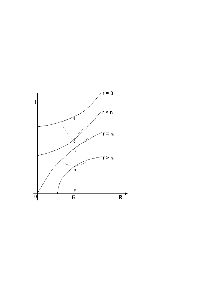
Figure 1: The straight line ${a-b-c-d-e}$ is the world line of an observer in the coordinates of the co-moving frame of reference. The curves represent the graphs of ${t_{(R)}}$ for various surfaces ${r={\rm\,const}}$. The dashed lines are light cones within which light can propagate. At the point $b$, the light cone intersects the surfaces ${r={\rm\,const}}$; hence, there is no horizon at this point. At the point $d$, the light cone passes above the curve ${r={\rm\,const}}$; hence, it intersects only the surfaces with ${r<r_{(R_{p},t)}}$; therefore, the point $d$ is below the horizon.

In Fig. 1, the straight vertical line ${a-b-c-d-e}$ denotes the world line of the particle $R_{p}$ in the coordinates of the co-moving frame of reference ${(R,t)}$ from the moment of rest ($a$) to the center of the system ($e$), where ${r=0}$. The solid curves passing through the points $e$, $d$, $c$, and $b$ represent the lines of constant values of ${r_{(R,t)}}$ for ${r=0}$, ${r<r_{h}}$, ${r=r_{h}}$ and ${r>r_{h}}$, respectively. The dashed lines with vertices at these points indicate cones within which light emitted by particle $R_{p}$ can propagate. Therefore, according to the above criterion, the horizon exists at the point where the cone is tangent to the line ${r={\rm\,const}}$; in Fig. 1, this line corresponds to the value ${r=r_{h}}$ (it passes through the point $c$).

The condition of constancy of the radius ${r_{(R,t)}}$ has the form:

$$dr=0=\dot{r}\,dt+r^{\prime}\,dR\,.$$ (11)

Hence, the tangent of the slope of the curve ${r={\rm\,const}}$ with respect to the axis $R$ is

$$\left.{dt\over dR}\right|_{r={\rm\,const}}=-{r^{\prime}\over\dot{r}}\,.$$ (12)

For the light cone, we have (by definition) ${ds^{2}=0}$, which, with regard to (1), yields

$$\left.{dt\over dR}\right|_{ds=0}=\sqrt{e^{\lambda-\nu}}\,.$$ (13)

Then, a criterion for the absence of a horizon is given by the condition:

$$\left.{dt\over dR}\right|_{ds=0}<\left.{dt\over dR}\right|_{r={\rm\,const}}\,.$$ (14)

Substituting (12) and (13) into this expression and introducing the physical velocity $V$ of the particle of matter, we rewrite this criterion as

$$V^{2}\equiv e^{\lambda-\nu}\left(\dot{r}/r^{\prime}\right)^{2}<1\,.$$ (15)

Introduce an element of proper (physical) time

$$d\tau\equiv\exp(\nu/2)dt\,.$$ (16)

a physical longitudinal distance $l$ and an element of physical length $dl$:

$$l_{(R,t)}\equiv\int\limits_{{}_{0}}^{R}e^{\lambda/2}{}_{(R,t)}\,dR\,,\quad dl\equiv\exp(\lambda/2)\,dR\,.$$ (17)

Then, the velocity of motion of matter with respect to the surfaces ${r={\rm\,const}}$ is given by

$$V=\left.{dl\over d\tau}\right|_{r={\rm\,const}}=\sqrt{e^{\lambda-\nu}}\left.{dR\over dt}\right|_{r={\rm\,const}}=\sqrt{e^{\lambda-\nu}}{\dot{r}\over r^{\prime}}\,.$$ (18)

This proves the assertion that the apparent horizon is formed at the moment when matter reaches the velocity ${|V|=1}$ with respect to the surface ${r={\rm\,const}}$.

4 GENERAL INTEGRALS OF MOTION

Integrating the first equation in (6) with regard to the initial conditions, we obtain

$$e^{\lambda}=e^{\lambda_{{}_{0}}}\left({R\over r}\right)^{4}\left({\varepsilon\over\varepsilon_{{}_{0}}}\right)^{2/\delta}\,.$$ (19)

The integration of the second equation in (6) yields

$$\nu=-2{1+\delta\over\delta}\ln(\varepsilon/\varepsilon_{{}_{\Lambda}})+c_{{}_{0}}(t)\,,$$ (20)

By an admissible transformation of time ${c_{{}_{0}}(t)}$, we can set the function ${c_{{}_{0}}(t)}$ equal to zero. Then,

$$\begin{array}[]{l}\nu=-2{1+\delta\over\delta}\ln(\varepsilon/\varepsilon_{{}_{\Lambda}})\end{array}$$ (21)

Then, condition (10) is fulfilled automatically as ${R\to\infty}$.

Let us rewrite Eq. (5) as

$$2{\dot{r}}^{\prime}=r^{\prime}\dot{\lambda}+\dot{r}\nu^{\prime}\,.$$ (22)

Determine ${\dot{\lambda}}$ from this equation and substitute it into Eq. (2). We obtain

$$8\pi\varepsilon r^{2}={1\over r^{\prime}}{d\over dR}\left(r-r{r^{\prime}}^{2}e^{-\lambda}+r{\dot{r}}^{2}e^{-\nu}\right)\,.$$ (23)

Let us introduce a new quantity that has the meaning of mass:

$$M_{(R,t)}\equiv\int\limits_{{}_{0}}^{R}4\pi\varepsilon r^{2}r^{\prime}\,dR\,,$$ (24)

Upon integrating Eq. (23), we can obtain two equations

$$2M=r\left(1-{r^{\prime}}^{2}e^{-\lambda}+{\dot{r}}^{2}e^{-\nu}\right)\,,\quad V^{2}=1-{e^{\lambda}\over{r^{\prime}}^{2}}\cdot\left(1-{2M\over r}\right)\,.$$ (25)

Hence, provided that ${\left.{r^{\prime}}^{2}e^{-\lambda}\right|_{r=r_{h}}\neq 0}$, the horizon radius is

$$r_{h}=2M_{(R_{h},t_{h})}\,.$$ (26)

Note that Eq. (3) coincides with Eq. (2) if we replace the time derivative by the derivative with respect to the coordinate (and vice versa), make the change ${\lambda\leftrightarrow\nu}$, and change the signs in the last terms of these equations. Then, by analogy, Eq. (23) can be rewritten as

$$-8\pi p_{\parallel}r^{2}={1\over\dot{r}}{d\over dt}\left(r-r{r^{\prime}}^{2}e^{-\lambda}+r{\dot{r}}^{2}e^{-\nu}\right)\,.$$ (27)

Integrating with respect to time and taking into account (25) and the initial conditions, we obtain

$$2M=2M_{{}_{0}}-\int\limits_{{}_{0}}^{t}8\pi p_{\parallel}r^{2}\dot{r}\,dt\,,$$ (28)

Here,

$$M_{{}_{0}}\equiv M_{(R,0)}\,,\quad S_{(R)}\equiv 2M_{{}_{0}}/R\,.$$ (29)

Formulas (24) and (25) yield an expression for the initial mass in the presence of a horizon:

$$2M_{{}_{0}}\equiv r_{1}+\int\limits_{r_{1}}^{R}8\pi\varepsilon_{{}_{0}}R^{2}\,dR\,,$$ (30)

where ${r_{{}_{1}}}$ is the initial radius of the horizon, which is defined by ${r_{{}_{1}}=r_{g}+\Lambda r_{{}_{1}}^{3}\approx r_{g}}$. Formula (28) determines a shift of the horizon in matter due to the work of pressure forces on the internal layers of matter (when matter is collapsed to the center). In [10], formula (28) was obtained for a particular case of ${w={\rm\,const}}$.

5 INITIAL CONDITIONS IN THE ABSENCE OF A HORIZON

Let us specify the initial conditions of the problem for a model in which there is no horizon at the initial moment. Using an admissible transformation ${R=R_{(\tilde{R})}}$, we can specify:

$$r_{{}_{0}}=R\quad\Longrightarrow\quad r^{\prime}_{{}_{0}}=1\,.$$ (31)

at the initial moment. In addition, we can specify the condition that matter is at rest at the initial moment:

$$\dot{\mu}_{{}_{0}}=0\,,\quad V_{{}_{0}}=0\,,\quad\dot{\lambda}_{{}_{0}}=0\,,\quad\dot{\nu}_{{}_{0}}=0\,.$$ (32)

Then, Eqs. (25) yield

$$\begin{array}[]{l}\lambda_{{}_{0}}=-\ln(1-S)\,,\end{array}$$ (33)

where

$$S\equiv 2M_{{}_{0}}/R\,,$$

this result does not depend on the choice of $\delta$.

6 INITIAL CONDITIONS IN THE PRESENCE OF A HORIZON

In this model, it is assumed that a horizon may exist at the initial moment; this assumption also concerns a purely vacuum solution with a $\Lambda$-term. Therefore, the initial conditions near the horizon deserve special mentioning.

The initial condition (31) is retained. With regard to (15), on the one hand, we have

$$V^{2}_{{}_{0}}{}_{(R)}=(\dot{r}_{{}_{0}})^{2}\cdot\left.\exp(\lambda_{{}_{0}}-\nu_{{}_{0}})\right|_{r_{h}}=1\,,$$

while, on the other hand,

$$\dot{r}_{{}_{0}}=0\,,\quad\left.e^{\lambda_{{}_{0}}}\right|_{r_{h}}\to\infty\,.$$

Therefore, we obtain indeterminacy of the form ${0\cdot\infty}$ on the horizon. Removing this indeterminacy, we obtain a physical distribution for velocity $V_{{}_{0}}$ at the initial moment:

$$|V_{{}_{0}}{}_{(R)}|=\left[\begin{array}[]{l}0\quad(R\neq r_{h})\,,\\ 1\quad(R=r_{h})\,.\end{array}\right.$$ (34)

i.e., the initial distribution of velocity represents a function with a ”punctured point.”

To validate formula (34), we modify the initial conditions: we assume that ${\dot{r}_{{}_{0}}\neq 0}$. Rewrite the second expression in (25) as

$$e^{-\lambda_{{}_{0}}}=1+\alpha-S\,,$$ (35)

where ${\alpha\equiv{\dot{r}_{{}_{0}}}^{2}e^{-\nu_{{}_{0}}}}$ is determined by the initial distribution of the velocity of matter.

Hence we obtain the following expression for the initial distribution of velocity:

$$V_{{}_{0}}^{2}={\alpha\over 1+\alpha-S}\,.$$ (36)

As ${\alpha\to 0}$, formula (36) turns into (34).

7 ANALYTICAL SOLUTION

Denote

$$y\equiv\ln(\varepsilon/\varepsilon_{{}_{\Lambda}})\,.$$ (37)

As ${\delta\to 0}$, we have ${\varepsilon\to\varepsilon_{{}_{\Lambda}}}$; therefore, ${y\to 0}$ as ${\delta\to 0}$.

Substituting ${\dot{\lambda}}$ and ${\nu^{\prime}}$ from Eqs. (6) into Eq. (22), we obtain

$$\delta\left({\dot{r}^{\prime}\over\dot{r}r^{\prime}}+{2\over r}\right)={\dot{y}\over\dot{r}}-(1+\delta){y^{\prime}\over r^{\prime}}\,.$$ (38)

Let us pass from the old coordinates ${(R,\,t)}$ to new coordinates ${(r,\,r_{h})}$, which are functions of the old coordinates. Applying a trivial mathematical transformation, we obtain

$${\dot{y}\over\dot{r}}-{y^{\prime}\over r^{\prime}}={\partial y\over\partial r_{h}}\left({\dot{r}_{h}\over\dot{r}}-{{r_{h}}^{\prime}\over r^{\prime}}\right).$$ (39)

In Section 10, we will show that, for small $\delta$, the variation of ${r_{h}}$ is also small (and proportional to $\delta$). Taking into account that ${y\to 0}$ as ${\delta\to 0}$, we can see that the right-hand side of (39) can be neglected as ${\delta\to 0}$. Then, Eq. (38) is rewritten as

$$\delta\left({\dot{r}^{\prime}\over\dot{r}r^{\prime}}+{2\over r}\right)\approx 0\,.$$ (40)

Now, let us find a solution to the Einstein equations in which the function $y$ (as well as $\varepsilon$ and $\nu$) depend explicitly only on the functions $r$ and ${r_{h}}$ and do not depend explicitly on $t$ and $R$. When the density of matter is defined so, the function ${\varepsilon(r)}$ is determined solely by the initial distribution of the density of matter.

As ${\delta\to 0}$, expressions (21) and (35) for $\nu_{{}_{0}}$ and $\lambda_{{}_{0}}$ must tend to ${\nu_{{}_{\Lambda}}}$ and ${\lambda_{{}_{\Lambda}}}$, respectively [see (8)], and $\alpha$ must tend to zero. Accordingly, we choose the energy density distribution as

$$\begin{array}[]{l}\varepsilon=\varepsilon_{{}_{\Lambda}}\left[1-{\delta\over 2}\ln\left(1+\alpha-{r_{h}\over r}\right)\right]\,,\\ \\ \nu=-2{1+\delta\over\delta}y\approx(1+\delta)\ln\left(1+\alpha-{r_{h}\over r}\right)\,.\end{array}$$ (41)

In the main approximation in $\delta$ with regard to the initial conditions, we obtain

$${\dot{r}^{\prime}\over r^{\prime}}\approx-{2\dot{r}\over r}\quad\Longrightarrow\quad r^{\prime}\approx\left(R\over r\right)^{2}\,.$$ (42)

Expression (30) yields

$$\begin{array}[]{l}2M_{{}_{0}}\approx r_{g}+\Lambda R^{3}-{3\over 2}\delta\Lambda r_{{}_{1}}^{3}\cdot I(R/r_{{}_{1}}-1)\,,\\ \\ I(x)=x^{3}\left[{\ln x\over 3}-{1\over 9}\right]+x^{2}\left[{\ln x\over 2}-{1\over 4}\right]+x\left[\ln x-1\right]-(x+1)^{3}\left[{\ln(x+1)\over 3}-{1\over 9}\right]-{1\over 9}\,,\\ \\ \lim\limits_{x\to 0}I(x)=x(\ln x-1)\to 0\,,\end{array}$$ (43)

where ${r_{{}_{1}}=r_{g}+\Lambda r_{{}_{1}}^{3}\approx r_{g}}$.

Taking into account that $\varepsilon$ depends explicitly only on $r$, we obtain the following expression from (28):

$$\begin{array}[]{l}2M=2M_{{}_{0}}(R)-(1+\delta)\int\limits_{r}^{R}8\pi\varepsilon r^{2}\,dr=2M_{{}_{0}}(r)-\delta\int\limits_{r}^{R}8\pi\varepsilon r^{2}\,dr\,.\end{array}$$ (44)

In the main approximation in $\delta$, formula (44) is rewritten as

$$2M\approx r_{g}+\Lambda r^{3}-\delta\Lambda\left[R^{3}-r^{3}+{3\over 2}r_{{}_{1}}^{3}\cdot I(r/r_{{}_{1}}-1)\right]\,.$$ (45)

From (19) and (35) we find

$$e^{\lambda}\approx{(R/r)^{4}\over 1+\alpha-S}\cdot\left[{1-{\delta\over 2}\ln\left(1+\alpha-r_{h}/r\right)\over 1-{\delta\over 2}\ln\left(1+\alpha-r_{h}/R\right)}\right]^{2/\delta}\,.$$ (46)

Hence, using (25) and applying the second remarkable limit to (46), we obtain

$$e^{\lambda}\approx{(R/r)^{4}\over 1+\alpha-S}\cdot\left({1+\alpha-r_{h}/R\over 1+\alpha-r_{h}/r}\right)\,,\quad V^{2}\approx 1-{1-2M/r\over 1+\alpha-S}\cdot\left({1+\alpha-r_{h}/R\over 1+\alpha-r_{h}/r}\right)\,.$$ (47)

According to the second expression in (25), the horizon radius $r_{h}$ is determined by the formula ${r_{h}=2M}$. Then, from (45) we find that

$$r_{h}-r_{{}_{1}}\approx-\delta\Lambda(R^{3}-r_{{}_{1}}^{3})\,.$$ (48)

as ${\delta\to 0}$. However, the solution obtained does not clearly indicate the direction of evolution (either collapsing or expansion). The direction of evolution is determined by the acceleration of matter at the initial moment.

8 ACCELERATION

Equations (3) and (35) yield the following expression for the second derivative of radius $r$ with respect to time $t$ at the initial moment:

$$2Re^{-\nu_{{}_{0}}}\ddot{r}_{{}_{0}}=(1+\delta)8\pi\varepsilon R^{2}+R\dot{r}_{{}_{0}}\dot{\nu}_{{}_{0}}e^{-\nu_{{}_{0}}}-S+R{\nu^{\prime}}_{{}_{0}}(1+\alpha-S)\,.$$ (49)

At the initial moment, the proper acceleration ${a=dV/d\tau}$ of the observer co-moving with matter is given by (see (18)):

$$a_{{}_{0}}=\ddot{r_{{}_{0}}}\cdot\exp(\lambda_{{}_{0}}/2-\nu_{{}_{0}})\,.$$ (50)

For small $\delta$, from (41) and (43) we obtain

$$\begin{array}[]{l}\nu_{{}_{0}}\approx(1+\delta)\ln\left(1+\alpha-S\right)\,,\\ \\ S\approx{r_{g}\over R}+\Lambda R^{2}-{3\over 2}\delta\Lambda{r_{{}_{1}}^{3}\over R}\cdot I(R/r_{{}_{1}}-1)\,,\\ \\ RS^{\prime}\approx-{r_{g}\over R}+2\Lambda R^{2}+{3\over 2}\delta\Lambda{r_{{}_{1}}^{3}\over R}\cdot\left[I(R/r_{{}_{1}}-1)-RI^{\prime}(R/r_{{}_{1}}-1)\right]\,.\end{array}$$ (51)

Let us rewrite (49) with regard to (51):

$$2Re^{-\nu_{{}_{0}}}\ddot{r}_{{}_{0}}\approx\delta\left[{r_{g}\over R}+\Lambda R^{2}+{3\over 2}\Lambda r_{{}_{1}}^{3}\cdot I^{\prime}\right]+\alpha{r_{g}/R-2\Lambda R^{2}+{3\over 2}\delta\Lambda r_{{}_{1}}^{3}(I^{\prime}-I/R)\over 1+\alpha-S}\,.$$ (52)

Hence, we can see that the acceleration vanishes (as it must) at ${\delta=0}$ (and ${\alpha=0}$).

For radii $R$ close to ${r_{{}_{1}}=r_{g}+\Lambda r_{{}_{1}}^{3}}$, the terms containing

$$I^{\prime}\approx\ln(R/r_{{}_{1}}-1)/r_{{}_{1}}<0,$$

prove to be dominant in (52). Denote

$$R_{cr}\approx r_{{}_{1}}\left[1+\exp\left(-{2\over 3\delta\Lambda r_{{}_{1}}R_{cr}}\right)\right]\approx r_{{}_{1}}\left[1+\exp\left(-{2\over 3\delta\Lambda r_{{}_{1}}^{2}}\right)\right]\approx r_{{}_{1}}\,,$$ (53)

Then, from (52) we find that, for $\delta>0$, matter expands at the initial moment when ${R>R_{cr}}$ and collapses when ${(R<R_{cr})}$ (in the close vicinity of the horizon).

9 CHARACTERISTIC EVOLUTION TIMES OF THE SYSTEM

In this section, we will not assume that $\delta$ is small. Then, neglecting $\alpha$ and using (49), we can obtain the following expression for the characteristic evolution time of the system:

$$T\sim\sqrt{r/|\ddot{r}|}.$$

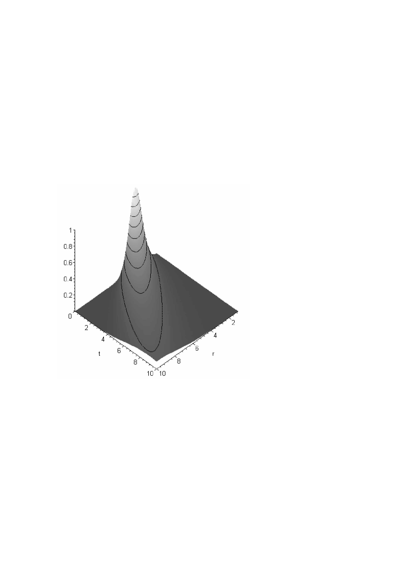
Figure 2: The behavior of a cloud of phantom matter. The cloud, which has the form of a Gaussian distribution when at rest, starts do expand with time. The vertical axis represents the energy density normalized to unity.

If the initial distribution of matter is characterized by large gradients, one can neglect all the terms in (49) except the terms containing ${R{\nu_{{}_{0}}}^{\prime}}$. Then, (49) and (50) yield

$$\ddot{r}_{{}_{0}}\approx{w\over\delta}({\varepsilon_{{}_{0}}}^{\prime}/\varepsilon_{{}_{0}})(1-S)(\varepsilon_{{}_{0}}/\varepsilon_{{}_{\Lambda}})^{2w/\delta}\,,\quad a_{{}_{0}}\approx{w\over\delta}({\varepsilon_{{}_{0}}}^{\prime}/\varepsilon_{{}_{0}})\sqrt{1-S}\,.$$ (54)

According to formulas (54), there are two alternative versions of the evolution of matter with the initial distribution in the form of a spherical layer with a local maximum of energy density:

1. In the case of phantom matter ${(\delta>0)}$, we obtain a expanding layer of matter (see Fig. 2).

2. When ${\delta<0}$, we obtain a collapsing layer of matter.

Note that the greater the density gradient, the faster the evolution. Apparently, these results can be generalized to a non-spherical model.

The characteristic evolution times corresponding to expressions (54) are given by

$$T_{1}\sim\sqrt{\left|(\delta/w)R\varepsilon_{{}_{0}}(\varepsilon_{{}_{\Lambda}}/\varepsilon_{{}_{0}})^{2w/\delta}\right|/\left|{\varepsilon_{{}_{0}}}^{\prime}(1-S)\right|}\,,\quad T_{2}\sim\sqrt{\left|(\delta/w)R\varepsilon_{{}_{0}}\right|/\left|{\varepsilon_{{}_{0}}}^{\prime}\sqrt{(1-S)}\right|}\,.$$ (55)

Here, $T_{1}$ is the evolution time for an infinitely distant observer, and $T_{2}$ is the evolution time for an observer that moves with matter.

To conclude this section, we consider the evolution of the domain that is characterized by the maximum energy density (a ”hump”; see Fig. 2). In this domain, ${R{\nu_{{}_{0}}}^{\prime}\approx 0}$; therefore, formulas (49) and (50) are rewritten in this domain as

$$\begin{array}[]{l}\ddot{r}_{{}_{0}}\approx\exp(\nu_{{}_{0}})\left[(1+\delta)\cdot 8\pi\varepsilon_{{}_{0}}R^{2}-S\right]/(2R)\,,\\ a_{{}_{0}}\approx\left[(1+\delta)\cdot 8\pi\varepsilon_{{}_{0}}R^{2}-S\right]/[2R\sqrt{1-S}]\,.\end{array}$$ (56)

For the initial distribution of matter similar to that shown in Fig. 2, we have

$$S=\frac{\int\limits_{{}_{{}_{0}}}^{{}_{R}}8\pi\varepsilon R^{2}\,dR}{R}<8\pi\varepsilon_{{}_{0}}R^{2},$$

at the maximum; therefore, the acceleration at this point proves to be positive; i.e., the ”hump”  decomposes and flies away from the center of the system (for any ${\delta>0}$).

10 DYNAMICS OF THE APPARENT HORIZON

Since all particles may intersect the horizon only in one direction, a strict correspondence is established between the coordinates ${R_{h}}$ and ${t_{h}}$ on the horizon. This means that ${R_{h}(t)}$ is a continuous and monotonically increasing function ${(\dot{R}_{h}>0)}$.

Consider formula (28) on the horizon. Differentiating this formula with respect to time, we obtain the following expression for the variation of the horizon radius:

$$\dot{r}_{h}=8\pi\varepsilon_{{}_{0}}R_{h}^{2}\cdot{dR_{h}\over dt}-8\pi w\varepsilon r^{2}\dot{r}\,.$$ (57)

Taking into account (12), we rewrite (57) as

$$\dot{r}_{h}=8\pi\varepsilon_{{}_{0}}R_{h}^{2}\cdot\dot{R}_{h}\cdot\left(1+wr^{\prime}\cdot{\varepsilon\over\varepsilon_{{}_{0}}}\cdot{r^{2}\over R^{2}}\right)$$ (58)

Consider two ways in which the horizon radius varies.

10.1 Test Matter

Consider the dynamics of the horizon for test matter (which negligibly affects the variations of the system and the radius of the horizon). For such matter, all functions must depend only on $r$. Otherwise, the metric in a static (fixed) frame of reference turns out to be nonstatic, which implies that it is affected by matter (i.e., the assumption that it is a test matter is violated).

Equation (11) determines the constancy of $r$, while the constancy of the metric component $\nu$ is given by

$$d\nu=0=\nu^{\prime}\,dR+\dot{\nu}\,dt\,.$$ (59)

Solving Eqs. (11) and (59) simultaneously, we obtain

$$\nu^{\prime}\dot{r}=\dot{\nu}r^{\prime}\,.$$ (60)

Equations (22) and (60) yield

$$2\dot{r^{\prime}}/r^{\prime}=\dot{\lambda}+\dot{\nu}\,.$$ (61)

Integrating this equation with regard to the initial conditions, we obtain

$$r^{\prime}=\sqrt{\exp{(\lambda-\lambda_{{}_{0}}+\nu-\nu_{{}_{0}})}}\,.$$ (62)

Hence, taking into account (19) and (21), we find

$$r^{\prime}={\varepsilon_{{}_{0}}\over\varepsilon}\cdot{R^{2}\over r^{2}}\,.$$ (63)

Now, formula (58) for the variation of the horizon radius is rewritten as

$$\dot{r}_{h}=8\pi\varepsilon_{{}_{0}}R_{h}^{2}\cdot\dot{R}_{h}\cdot(1+w)\,.$$ (64)

Thus, for ${w<-1}$, we have ${\dot{r}_{h}<0}$; i.e., in the case of test matter, the horizon radius decreases, and the black hole is ”dissolved”  in phantom matter.

In formula (64), the fact that matter is test manifests itself in that the quantity ${8\pi\varepsilon_{{}_{0}}R^{2}}$ is extremely small, ${8\pi\varepsilon_{{}_{0}}R^{2}<<<1}$. This result was predicted and proved for the static frame of reference (a frame of reference fixed with respect to distant stars) in [5].

10.2 Nontest Matter

Formula (64) can be generalized to nontest matter. To this end, it suffices to notice that, when the horizon radius is constant, the metric coefficients on the horizon are also time-independent (the gravitational field at radius $r$ is determined only by the mass within this radius, i.e., by the mass within the horizon radius in the case considered). Therefore, the following relation must hold for ${\dot{r}_{h}=0}$:

$$d\nu|_{r_{h}}=0.$$

Using this in expression (59) on the horizon, we obtain the same result (64). Hence, if the accretion of matter does not change the horizon radius, then the equality ${w=-1}$ must hold.

$$\left.d\nu\right|_{r_{h}}=\dot{\nu}\,dt+\nu^{\prime}\,dR\,.$$ (65)

Solving Eqs. (11) and (65) simultaneously, we obtain

$$\nu^{\prime}\dot{r}=\dot{\nu}r^{\prime}-r^{\prime}\,\left.{d\nu\over dt}\right|_{r=r_{h}={\rm\,const}}\,.$$ (66)

which is an analog of Eq. (60). Equations (66) and (22) yield

$$2\dot{r^{\prime}}/r^{\prime}=\dot{\lambda}+\dot{\nu}-\left.{d\nu\over dt}\right|_{r=r_{h}={\rm\,const}}\,.$$ (67)

Integration of this equation with the initial conditions yields analog of Eq. (62):

$$r^{\prime}=\sqrt{\exp(\lambda-\lambda_{{}_{0}}+\nu-\nu_{{}_{0}})\cdot\exp\left(\nu_{[1]}-\nu_{[2]}\right)}\,,$$ (68)

Here, the following notation is used: ${[1]\equiv(r_{h},0)}$ and ${[2]\equiv(R_{h},t_{h})}$; ${r_{[1]}=r_{[2]}=r_{h}}$. An expression for the variation of the horizon radius is obtained analogously (64):

$$\dot{r}_{h}=8\pi\varepsilon_{{}_{0}}R_{h}^{2}\cdot\dot{R}_{h}\cdot[1+w\Psi]\,,\quad\Psi\equiv\sqrt{\exp\left(\nu_{[1]}-\nu_{[2]}\right)}=\left({\varepsilon_{[1]}\over\varepsilon_{[2]}}\right)^{w/\delta}\,.$$ (69)

These are exact expression independent of $\delta$. Thus, the direction in which the horizon is shifted depends on the initial conditions of the distribution of matter. The condition under which the horizon radius decreases is given by ${w\Psi<-1}$.

For a matter distribution that depends explicitly only on $r$, we obtain ${\Psi=1}$. Then, formulas (13), (41), (47) and (69) yield

$$\dot{r}_{h}\approx-3\left({\delta\over\sqrt{\alpha}}\right)\Lambda r_{h}^{2}(1+\alpha-S)^{3/2}\quad\Longrightarrow\quad T_{r_{{}_{1}}\to r_{h}}\approx{\sqrt{\alpha}(r_{{}_{1}}-r_{h})\over 3|\delta|\Lambda r_{{}_{1}}r_{h}(1+\alpha-S)^{3/2}}\,.$$ (70)

This formula shows that, in the general case, the ”dissolution”  degree of a black hole for small $\delta$ is rather small.

11 CONCLUSIONS

The main conclusion of the present study is the confirmation of the conjecture on a possible decrease of the horizon radius (solution) of a black hole.

Note that, at infinity, there is no paradox related to this phenomenon. In the absence of matter, the metric at infinity persists to be Schwarzschild (with a $\Lambda$-term). Accordingly, the total mass of the whole system related to this metric remains constant. The point is that the mass and energy are redistributed in space during evolution: an external wave of phantom matter removes the mass and energy that correspond to the initial black hole (which is ”dissolved”  under the action of the internal wave of phantom matter). If the black hole is not ”dissolved”  completely, the total energy of the system is composed of the mass of the changed black hole and the energy of the external wave of phantom matter.

   

ACKNOWLEDGMENTS:
I am grateful to I.D. Novikov and N.S. Kardashev for discussing various questions while preparing this article.

References

• [1] M. Visser, Lorential Wormholes: from Einstein to Hawking, AIP, Woodbury, N.Y., (1996)
• [2] Shatskiy Alexander, Astron. Zh., 84, 99, (2007) [Astron. Rep., 51, 81, (2007)]
• [3] V. P. Frolov and I. D. Novikov, Black Hole Physics: Basic Concepts and New Developments, (Kluwer, Dordrecht, 1998)
• [4] Shatskiy Alexander, Astron. Zh., 81, 579, (2004) [Astron. Rep., 48, 525, (2004)]
• [5] Babichev E., Dokuchaev V., and Eroshenko Y., grqc/0507119
• [6] Khabibullin A.R., Khusnutdinov N.R., and Sushkov S.V., hep-th/0510232
• [7] Kardashev N.S., Novikov I.D., and Shatskiy Alexander, Astron. Zh., 83, 675, (2006) [Astron. Rep., 50, 601, (2006)]
• [8] Landau L.D. and Lifshitz E.M., Course of Theoretical Physics, Vol. 2: The Classical Theory of Fields, 7th ed. (Nauka, Moscow, 1988; Pergamon, Oxford, 1975)
• [9] Wyman M., Phys. Rev., 75, 1930 (1949)
• [10] Shatskiy Alexander and Andreev A.Yu., Zh. Eksp. Teor. Fiz. 116, 353, (1999) [JETP, 89, 189, (1999)]