A Tutorial on Spectral Clustering
The original publication is available at www.springer.com.)
Abstract
In recent years, spectral clustering has become one of the most popular modern clustering algorithms. It is simple to implement, can be solved efficiently by standard linear algebra software, and very often outperforms traditional clustering algorithms such as the k-means algorithm. On the first glance spectral clustering appears slightly mysterious, and it is not obvious to see why it works at all and what it really does. The goal of this tutorial is to give some intuition on those questions. We describe different graph Laplacians and their basic properties, present the most common spectral clustering algorithms, and derive those algorithms from scratch by several different approaches. Advantages and disadvantages of the different spectral clustering algorithms are discussed.
Keywords: spectral clustering; graph Laplacian
1 Introduction
Clustering is one of the most widely used techniques for exploratory data
analysis, with applications ranging from statistics, computer science,
biology to social sciences or psychology. In virtually
every scientific field dealing with empirical data, people attempt to get
a first impression on their data by trying to identify groups of
“similar behavior” in their data.
In this article we would like to introduce the reader to the family of
spectral clustering algorithms. Compared to the “traditional
algorithms” such as -means or single linkage, spectral clustering
has many fundamental advantages. Results obtained by spectral
clustering often outperform the traditional approaches, spectral
clustering is very simple to
implement and can be solved efficiently by standard linear algebra methods.
This tutorial is set up as a self-contained introduction to spectral clustering. We derive spectral clustering from scratch and present different points of view to why spectral clustering works. Apart from basic linear algebra, no particular mathematical background is required by the reader. However, we do not attempt to give a concise review of the whole literature on spectral clustering, which is impossible due to the overwhelming amount of literature on this subject. The first two sections are devoted to a step-by-step introduction to the mathematical objects used by spectral clustering: similarity graphs in Section 2, and graph Laplacians in Section 3. The spectral clustering algorithms themselves will be presented in Section 4. The next three sections are then devoted to explaining why those algorithms work. Each section corresponds to one explanation: Section 5 describes a graph partitioning approach, Section 6 a random walk perspective, and Section 7 a perturbation theory approach. In Section 8 we will study some practical issues related to spectral clustering, and discuss various extensions and literature related to spectral clustering in Section 9.
2 Similarity graphs
Given a set of data points and some notion of similarity between all pairs of data points and , the intuitive goal of clustering is to divide the data points into several groups such that points in the same group are similar and points in different groups are dissimilar to each other. If we do not have more information than similarities between data points, a nice way of representing the data is in form of the similarity graph . Each vertex in this graph represents a data point . Two vertices are connected if the similarity between the corresponding data points and is positive or larger than a certain threshold, and the edge is weighted by . The problem of clustering can now be reformulated using the similarity graph: we want to find a partition of the graph such that the edges between different groups have very low weights (which means that points in different clusters are dissimilar from each other) and the edges within a group have high weights (which means that points within the same cluster are similar to each other). To be able to formalize this intuition we first want to introduce some basic graph notation and briefly discuss the kind of graphs we are going to study.
2.1 Graph notation
Let be an undirected graph with vertex set . In the following we assume that the graph is weighted, that is each edge between two vertices and carries a non-negative weight . The weighted adjacency matrix of the graph is the matrix . If this means that the vertices and are not connected by an edge. As is undirected we require . The degree of a vertex is defined as
Note that, in fact, this sum only runs over all vertices adjacent to , as for all other vertices the weight is 0. The degree matrix is defined as the diagonal matrix with the degrees on the diagonal. Given a subset of vertices , we denote its complement by . We define the indicator vector as the vector with entries if and otherwise. For convenience we introduce the shorthand notation for the set of indices , in particular when dealing with a sum like . For two not necessarily disjoint sets we define
We consider two different ways of measuring the “size” of a subset :
Intuitively, measures the size of by its number of vertices, while measures the size of by summing over the weights of all edges attached to vertices in . A subset of a graph is connected if any two vertices in can be joined by a path such that all intermediate points also lie in . A subset is called a connected component if it is connected and if there are no connections between vertices in and . The nonempty sets form a partition of the graph if and .
2.2 Different similarity graphs
There are several popular constructions to transform a given set
of data points with pairwise similarities
or pairwise distances into a graph. When constructing
similarity graphs the goal is to model the local neighborhood
relationships between the data points.
The -neighborhood graph: Here we connect all points
whose pairwise distances are smaller than . As the distances
between all connected points are roughly of the same scale (at most
), weighting the edges would not incorporate more information
about the data to the graph. Hence, the -neighborhood graph is
usually considered as an unweighted graph.
-nearest neighbor graphs: Here the goal is to connect vertex
with vertex if is among the -nearest neighbors of
. However, this definition leads to a directed graph, as the
neighborhood relationship is not symmetric. There are two ways of
making this graph undirected. The first way is to simply ignore the
directions of the edges, that is we connect and with an
undirected
edge if is among the -nearest neighbors of or if
is among the -nearest neighbors of . The resulting graph
is what is usually called the -nearest neighbor graph. The
second choice is to connect vertices and if both is
among the -nearest neighbors of and is among the
-nearest neighbors of . The resulting graph is called the mutual -nearest neighbor graph. In both cases, after connecting
the appropriate vertices we weight the edges by the similarity of their endpoints.
The fully connected graph: Here we simply connect all points
with positive similarity with each other, and we weight all edges by
. As the graph should represent the local neighborhood
relationships, this construction is only useful if the
similarity function itself models local neighborhoods. An example for
such a similarity function is the Gaussian similarity function
, where
the parameter controls the width of the neighborhoods. This
parameter plays a similar role as the parameter in case
of the -neighborhood graph.
All graphs mentioned above are regularly used in spectral
clustering. To our knowledge, theoretical results on the question how
the choice of the similarity graph influences the spectral clustering
result do not exist. For a discussion of the behavior of
the different graphs we refer to Section 8.
3 Graph Laplacians and their basic properties
The main tools for spectral clustering are graph Laplacian
matrices. There exists a whole field dedicated to the study of those
matrices, called spectral graph theory (e.g., see ?, ?). In
this section we want to define different graph Laplacians and point
out their most important properties. We will carefully distinguish
between different variants of graph Laplacians. Note that in the
literature there is no unique convention which matrix exactly is
called “graph Laplacian”.
Usually, every author just calls “his” matrix the graph
Laplacian. Hence, a lot of care is needed when reading literature on
graph Laplacians.
In the following we always assume that is an undirected, weighted graph with weight matrix , where . When using eigenvectors of a matrix, we will not necessarily assume that they are normalized. For example, the constant vector and a multiple for some will be considered as the same eigenvectors. Eigenvalues will always be ordered increasingly, respecting multiplicities. By “the first eigenvectors” we refer to the eigenvectors corresponding to the smallest eigenvalues.
3.1 The unnormalized graph Laplacian
The unnormalized graph Laplacian matrix is defined as
An overview over many of its properties can be found in ? (?, ?). The following proposition summarizes the most important facts needed for spectral clustering.
Proposition 1 (Properties of )
The matrix satisfies the following properties:
-
1.
For every vector we have
-
2.
is symmetric and positive semi-definite.
-
3.
The smallest eigenvalue of is 0, the corresponding eigenvector is the constant one vector .
-
4.
has non-negative, real-valued eigenvalues .
Proof.
Part (1): By the definition of ,
Part (2): The symmetry of follows directly from the symmetry of
and . The positive semi-definiteness is a direct consequence of
Part (1), which shows that for all .
Part (3): Obvious.
Part (4) is a direct consequence of Parts (1) - (3).
Note that the unnormalized graph Laplacian does not depend on the
diagonal elements of the adjacency matrix . Each adjacency matrix which
coincides with on all off-diagonal positions leads to the same
unnormalized graph Laplacian . In particular, self-edges in a
graph do not change the corresponding graph Laplacian.
The unnormalized graph Laplacian and its eigenvalues and eigenvectors can be used to describe many properties of graphs, see ? (?, ?). One example which will be important for spectral clustering is the following:
Proposition 2 (Number of connected components and the spectrum of )
Let be an undirected graph with non-negative weights. Then the multiplicity of the eigenvalue of equals the number of connected components in the graph. The eigenspace of eigenvalue is spanned by the indicator vectors of those components.
Proof. We start with the case , that is the graph is connected. Assume that is an eigenvector with eigenvalue . Then we know that
As the weights are non-negative, this sum can only vanish if
all terms vanish. Thus, if two vertices
and are connected (i.e., ), then needs to
equal . With this argument we can see that needs to be
constant for all vertices which can be connected by a path in the
graph. Moreover, as all vertices of a connected component in an
undirected graph can be connected by a path, needs to be constant
on the whole connected component. In a graph consisting of only one
connected component we thus only have the constant one vector
as eigenvector with eigenvalue 0, which obviously is the
indicator vector of the connected component.
Now consider the case of connected components. Without loss of generality we assume that the vertices are ordered according to the connected components they belong to. In this case, the adjacency matrix has a block diagonal form, and the same is true for the matrix :
Note that each of the blocks is a proper graph Laplacian on its
own, namely the Laplacian corresponding to the subgraph of the -th connected
component.
As it is the case for all block diagonal matrices, we know that the
spectrum of is given by the union of the spectra of , and the
corresponding eigenvectors of are the eigenvectors of ,
filled with 0 at the positions of the other blocks.
As each is a graph Laplacian of a connected graph, we know that
every has eigenvalue 0 with multiplicity 1, and the
corresponding eigenvector is the constant one vector on the -th
connected component. Thus, the matrix has as many eigenvalues
as there are connected components, and the corresponding
eigenvectors are the indicator vectors of the connected components.
3.2 The normalized graph Laplacians
There are two matrices which are called normalized graph Laplacians in the literature. Both matrices are closely related to each other and are defined as
We denote the first matrix by as it is a symmetric matrix, and
the second one by as it is closely related to a random walk.
In the following we summarize several properties of and
. The standard reference for normalized graph Laplacians is ? (?).
Proposition 3 (Properties of and )
The normalized Laplacians satisfy the following properties:
-
1.
For every we have
-
2.
is an eigenvalue of with eigenvector if and only if is an eigenvalue of with eigenvector .
-
3.
is an eigenvalue of with eigenvector if and only if and solve the generalized eigenproblem .
-
4.
is an eigenvalue of with the constant one vector as eigenvector. is an eigenvalue of with eigenvector .
-
5.
and are positive semi-definite and have non-negative real-valued eigenvalues .
Proof.
Part (1) can be proved similarly to Part (1) of Proposition
1.
Part (2) can be seen immediately by multiplying the eigenvalue
equation with from the left and
substituting .
Part (3) follows directly by multiplying the eigenvalue equation with from the left.
Part (4): The first statement is obvious as , the second statement follows from (2).
Part (5): The statement about follows from (1),
and then the statement about follows from (2).
As it is the case for the unnormalized graph Laplacian, the multiplicity of the eigenvalue 0 of the normalized graph Laplacian is related to the number of connected components:
Proposition 4 (Number of connected components and spectra of and )
Let be an undirected graph with non-negative weights. Then the multiplicity of the eigenvalue of both and equals the number of connected components in the graph. For , the eigenspace of is spanned by the indicator vectors of those components. For , the eigenspace of is spanned by the vectors .
4 Spectral Clustering Algorithms
Now we would like to state the most common spectral clustering algorithms. For references and the history of spectral clustering we refer to Section 9. We assume that our data consists of “points” which can be arbitrary objects. We measure their pairwise similarities by some similarity function which is symmetric and non-negative, and we denote the corresponding similarity matrix by .
Unnormalized spectral clustering
Input: Similarity matrix , number of clusters to construct.
Construct a similarity graph by one of the ways described in
Section 2. Let be its weighted adjacency matrix.
Compute the unnormalized Laplacian .
Compute the first eigenvectors of .
Let be the matrix containing the vectors as
columns.
For , let be the vector corresponding to the -th
row of .
Cluster the points in with the -means
algorithm into clusters .
Output: Clusters with .
There are two different versions of normalized spectral clustering, depending which of the normalized graph Laplacians is used. We name both algorithms after two popular papers, for more references and history please see Section 9.
Normalized spectral clustering according to
? (?)
Input: Similarity matrix , number of clusters to construct.
Construct a similarity graph by one of the ways described in
Section 2. Let be its weighted adjacency matrix.
Compute the unnormalized Laplacian .
Compute the first generalized eigenvectors of the
generalized eigenproblem .
Let be the matrix containing the vectors as
columns.
For , let be the vector corresponding to the -th
row of .
Cluster the points in with the -means
algorithm into clusters .
Output: Clusters with .
Note that this algorithm uses the generalized eigenvectors of ,
which according to Proposition 3 correspond to the
eigenvectors of the matrix . So in fact, the
algorithm works with eigenvectors of the normalized Laplacian , and hence is called
normalized spectral clustering.
The next algorithm also uses a normalized Laplacian, but this time the
matrix instead of . As we will see, this algorithm needs
to introduce an additional row normalization step which is not needed
in the other algorithms. The reasons will
become clear in Section 7.
Normalized spectral clustering according to
? (?)
Input: Similarity matrix , number of clusters to construct.
Construct a similarity graph by one of the ways described in
Section 2. Let be its weighted adjacency matrix.
Compute the normalized Laplacian .
Compute the first eigenvectors
of
.
Let be the matrix containing the vectors as
columns.
Form the matrix from by normalizing the rows to norm 1,
that is set .
For , let be the vector corresponding to the -th
row of .
Cluster the points with the -means
algorithm into clusters .
Output: Clusters with .
All three algorithms stated above look rather similar, apart from the
fact that they use three different graph Laplacians. In all three
algorithms, the main trick is to change the representation of the
abstract data points to points . It is due to the
properties of the graph Laplacians that this change of representation
is useful. We will see in the next sections that this change of
representation enhances the cluster-properties in the data, so that
clusters can be trivially detected in the new representation. In
particular, the simple -means clustering algorithm has no
difficulties to detect the clusters in this new representation.
Readers not familiar with -means can read up on this algorithm in numerous text books, for
example in ? (?).
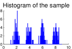
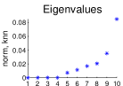
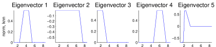
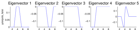
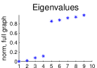
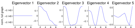
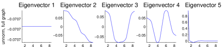
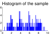
Before we dive into the theory of spectral clustering, we would like to illustrate its principle on a very simple toy example. This example will be used at several places in this tutorial, and we chose it because it is so simple that the relevant quantities can easily be plotted. This toy data set consists of a random sample of 200 points drawn according to a mixture of four Gaussians. The first row of Figure 1 shows the histogram of a sample drawn from this distribution (the -axis represents the one-dimensional data space). As similarity function on this data set we choose the Gaussian similarity function with . As similarity graph we consider both the fully connected graph and the -nearest neighbor graph. In Figure 1 we show the first eigenvalues and eigenvectors of the unnormalized Laplacian and the normalized Laplacian . That is, in the eigenvalue plot we plot vs. (for the moment ignore the dashed line and the different shapes of the eigenvalues in the plots for the unnormalized case; their meaning will be discussed in Section 8.5). In the eigenvector plots of an eigenvector we plot vs. (note that in the example chosen is simply a real number, hence we can depict it on the -axis). The first two rows of Figure 1 show the results based on the -nearest neighbor graph. We can see that the first four eigenvalues are 0, and the corresponding eigenvectors are cluster indicator vectors. The reason is that the clusters form disconnected parts in the -nearest neighbor graph, in which case the eigenvectors are given as in Propositions 2 and 4. The next two rows show the results for the fully connected graph. As the Gaussian similarity function is always positive, this graph only consists of one connected component. Thus, eigenvalue 0 has multiplicity 1, and the first eigenvector is the constant vector. The following eigenvectors carry the information about the clusters. For example in the unnormalized case (last row), if we threshold the second eigenvector at 0, then the part below 0 corresponds to clusters 1 and 2, and the part above 0 to clusters 3 and 4. Similarly, thresholding the third eigenvector separates clusters 1 and 4 from clusters 2 and 3, and thresholding the fourth eigenvector separates clusters 1 and 3 from clusters 2 and 4. Altogether, the first four eigenvectors carry all the information about the four clusters. In all the cases illustrated in this figure, spectral clustering using -means on the first four eigenvectors easily detects the correct four clusters.
5 Graph cut point of view
The intuition of clustering is to separate points in different groups
according to their similarities. For data given in form of a
similarity graph, this problem can be restated as follows: we want to
find a partition of the graph such that the edges between different
groups have a very low weight (which means that points in different
clusters are dissimilar from each other) and the edges within a group
have high weight (which means that points within the same cluster are
similar to each other). In this section we will see how spectral
clustering can be derived as an approximation to such graph
partitioning problems.
Given a similarity graph with adjacency matrix , the simplest and most direct way to construct a partition of the graph is to solve the mincut problem. To define it, please recall the notation and for the complement of . For a given number of subsets, the mincut approach simply consists in choosing a partition which minimizes
Here we introduce the factor for notational consistency, otherwise we would count each edge twice in the cut. In particular for , mincut is a relatively easy problem and can be solved efficiently, see ? (?) and the discussion therein. However, in practice it often does not lead to satisfactory partitions. The problem is that in many cases, the solution of mincut simply separates one individual vertex from the rest of the graph. Of course this is not what we want to achieve in clustering, as clusters should be reasonably large groups of points. One way to circumvent this problem is to explicitly request that the sets are “reasonably large”. The two most common objective functions to encode this are (?, ?) and the normalized cut (?, ?). In , the size of a subset of a graph is measured by its number of vertices , while in the size is measured by the weights of its edges . The definitions are:
Note that both objective functions take a small value if the clusters are not too small. In particular, the minimum of the function is achieved if all coincide, and the minimum of is achieved if all coincide. So what both objective functions try to achieve is that the clusters are “balanced”, as measured by the number of vertices or edge weights, respectively. Unfortunately, introducing balancing conditions makes the previously simple to solve mincut problem become NP hard, see ? (?) for a discussion. Spectral clustering is a way to solve relaxed versions of those problems. We will see that relaxing leads to normalized spectral clustering, while relaxing leads to unnormalized spectral clustering (see also the tutorial slides by ? (?)).
5.1 Approximating for
Let us start with the case of and , because the relaxation is easiest to understand in this setting. Our goal is to solve the optimization problem
| (1) |
We first rewrite the problem in a more convenient form. Given a subset we define the vector with entries
| (2) |
Now the objective function can be conveniently rewritten using the unnormalized graph Laplacian. This is due to the following calculation:
Additionally, we have
In other words, the vector as defined in Equation (2) is orthogonal to the constant one vector . Finally, note that satisfies
Altogether we can see that the problem of minimizing (1) can be equivalently rewritten as
| (3) |
This is a discrete optimization problem as the entries of the solution vector are only allowed to take two particular values, and of course it is still NP hard. The most obvious relaxation in this setting is to discard the discreteness condition and instead allow that takes arbitrary values in . This leads to the relaxed optimization problem
| (4) |
By the Rayleigh-Ritz theorem (e.g., see Section 5.5.2. of ?, ?) it can be seen immediately that the solution of this problem is given by the vector which is the eigenvector corresponding to the second smallest eigenvalue of (recall that the smallest eigenvalue of is 0 with eigenvector ). So we can approximate a minimizer of by the second eigenvector of . However, in order to obtain a partition of the graph we need to re-transform the real-valued solution vector of the relaxed problem into a discrete indicator vector. The simplest way to do this is to use the sign of as indicator function, that is to choose
However, in particular in the case of treated below, this heuristic is too simple. What most spectral clustering algorithms do instead is to consider the coordinates as points in and cluster them into two groups by the -means clustering algorithm. Then we carry over the resulting clustering to the underlying data points, that is we choose
This is exactly the unnormalized spectral clustering algorithm
for the case
of .
5.2 Approximating for arbitrary
The relaxation of the minimization problem in the case of a general value follows a similar principle as the one above. Given a partition of into sets , we define indicator vectors by
| (5) |
Then we set the matrix as the matrix containing those indicator vectors as columns. Observe that the columns in are orthonormal to each other, that is . Similar to the calculations in the last section we can see that
Moreover, one can check that
Combining those facts we get
where denotes the trace of a matrix. So the problem of minimizing can be rewritten as
Similar to above we now relax the problem by allowing the entries of the matrix to take arbitrary real values. Then the relaxed problem becomes:
This is the standard form of a trace minimization problem, and again a version of the Rayleigh-Ritz theorem (e.g., see Section 5.2.2.(6) of ?, ?) tells us that the solution is given by choosing as the matrix which contains the first eigenvectors of as columns. We can see that the matrix is in fact the matrix used in the unnormalized spectral clustering algorithm as described in Section 4. Again we need to re-convert the real valued solution matrix to a discrete partition. As above, the standard way is to use the -means algorithms on the rows of . This leads to the general unnormalized spectral clustering algorithm as presented in Section 4.
5.3 Approximating
Techniques very similar to the ones used for can be used to derive normalized spectral clustering as relaxation of minimizing . In the case we define the cluster indicator vector by
| (6) |
Similar to above one can check that , , and . Thus we can rewrite the problem of minimizing by the equivalent problem
| (7) |
Again we relax the problem by allowing to take arbitrary real values:
| (8) |
Now we substitute . After substitution, the problem is
| (9) |
Observe that , is
the first eigenvector of , and is a constant. Hence,
Problem (9) is in the form
of the standard Rayleigh-Ritz theorem, and its solution is given
by the second eigenvector of . Re-substituting
and using Proposition 3 we see that is the
second eigenvector of , or equivalently the generalized
eigenvector of .
For the case of finding clusters, we define the indicator vectors by
| (10) |
Then we set the matrix as the matrix containing those indicator vectors as columns. Observe that , , and . So we can write the problem of minimizing as
Relaxing the discreteness condition and substituting we obtain the relaxed problem
| (11) |
Again this is the standard trace minimization problem which is solved
by the matrix which contains the first eigenvectors of
as columns. Re-substituting and using Proposition
3 we see that the solution consists of the first
eigenvectors of the matrix , or the first generalized
eigenvectors of . This yields the normalized
spectral clustering algorithm according to ? (?).
5.4 Comments on the relaxation approach
There are several comments we should make about this derivation of spectral clustering. Most importantly, there is no guarantee whatsoever on the quality of the solution of the relaxed problem compared to the exact solution. That is, if is the exact solution of minimizing , and is the solution constructed by unnormalized spectral clustering, then can be arbitrary large. Several examples for this can be found in ? (?). For instance, the authors consider a very simple class of graphs called “cockroach graphs”. Those graphs essentially look like a ladder, with a few rimes removed, see Figure 2.
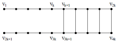
Obviously, the ideal for just cuts the ladder by a vertical
cut such that and
. This
cut is perfectly balanced with and . However, by studying the properties of the second eigenvector
of the unnormalized graph Laplacian of cockroach graphs the authors
prove that unnormalized spectral clustering always cuts horizontally
through the ladder, constructing the sets and . This also results in a
balanced cut, but now we cut edges instead of just . So
, while . This
means that compared to the optimal cut, the
value obtained by spectral clustering is
times worse, that is a factor in the order of . Several other papers investigate the quality of the clustering
constructed by spectral clustering, for example ? (?) (for
unnormalized spectral clustering) and
? (?) (for normalized spectral clustering).
In general it is known that efficient algorithms to approximate
balanced graph cuts up to a constant factor do not exist. To the
contrary, this approximation problem can be NP hard itself
(?, ?).
Of course, the relaxation we discussed above is not unique. For
example, a completely different relaxation which leads to a
semi-definite program is derived in ? (?), and there might
be many other useful relaxations.
The reason why the spectral relaxation is so appealing is not that it
leads to particularly good solutions. Its popularity is mainly due to the fact that it results in
a standard linear algebra problem which is simple to solve.
6 Random walks point of view
Another line of argument to explain spectral clustering is based on random walks on the similarity graph. A random walk on a graph is a stochastic process which randomly jumps from vertex to vertex. We will see below that spectral clustering can be interpreted as trying to find a partition of the graph such that the random walk stays long within the same cluster and seldom jumps between clusters. Intuitively this makes sense, in particular together with the graph cut explanation of the last section: a balanced partition with a low cut will also have the property that the random walk does not have many opportunities to jump between clusters. For background reading on random walks in general we refer to ? (?) and ? (?), and for random walks on graphs we recommend ? (?) and ? (?). Formally, the transition probability of jumping in one step from vertex to vertex is proportional to the edge weight and is given by . The transition matrix of the random walk is thus defined by
If the graph is connected and non-bipartite, then the random walk always possesses a unique stationary distribution , where . Obviously there is a tight relationship between and , as . As a consequence, is an eigenvalue of with eigenvector if and only if is an eigenvalue of with eigenvector . It is well known that many properties of a graph can be expressed in terms of the corresponding random walk transition matrix , see ? (?) for an overview. From this point of view it does not come as a surprise that the largest eigenvectors of and the smallest eigenvectors of can be used to describe cluster properties of the graph.
Random walks and
A formal equivalence between and transition probabilities of the random walk has been observed in ? (?).
Proposition 5 ( via transition probabilities)
Let be connected and non bi-partite. Assume that we run the random walk starting with in the stationary distribution . For disjoint subsets , denote by . Then:
Proof. First of all observe that
Using this we obtain
Now the proposition follows directly with the definition of .
This proposition leads to a nice interpretation of , and hence of normalized spectral clustering. It tells us that when minimizing , we actually look for a cut through the graph such that a random walk seldom transitions from to and vice versa.
The commute distance
A second connection between random walks and graph Laplacians
can be made via the commute distance on the graph. The commute
distance (also called resistance distance) between two
vertices and is the expected time it takes the random walk to
travel from vertex to vertex and back
(?, ?, ?). The commute distance has several nice
properties which make it particularly appealing for machine
learning. As opposed to the shortest path distance on a graph, the
commute distance between two vertices decreases if there are many
different short ways to get from vertex to vertex . So instead
of just looking for the one shortest path, the commute distance looks
at the set of short paths. Points which are connected by a short path
in the graph and lie in the same high-density region of the graph are
considered closer to each other than points which are connected by a
short path but lie in different high-density regions of the graph. In
this sense, the commute distance seems particularly well-suited to be
used for clustering purposes.
Remarkably, the commute distance on a graph can be computed with the help of the generalized inverse (also called pseudo-inverse or Moore-Penrose inverse) of the graph Laplacian . In the following we denote as the -th unit vector. To define the generalized inverse of , recall that by Proposition 1 the matrix can be decomposed as where is the matrix containing all eigenvectors as columns and the diagonal matrix with the eigenvalues on the diagonal. As at least one of the eigenvalues is 0, the matrix is not invertible. Instead, we define its generalized inverse as where the matrix is the diagonal matrix with diagonal entries if and if . The entries of can be computed as . The matrix is positive semi-definite and symmetric. For further properties of see ? (?).
Proposition 6 (Commute distance)
Let a connected, undirected graph. Denote by the commute distance between vertex and vertex , and by the generalized inverse of . Then we have:
This result has been published by ? (?), where it has been
proved by methods of electrical network theory. For a proof using
first step analysis for random walks see ? (?).
There also exist other ways to express the commute distance with the
help of graph Laplacians. For example a method in terms of
eigenvectors of the normalized Laplacian can be found as
Corollary 3.2 in ? (?), and a method computing the commute
distance with the help of determinants of certain sub-matrices of
can be found in ? (?).
Proposition 6 has an important consequence. It shows
that can be considered as a Euclidean distance
function on the vertices of the graph. This means that we can
construct an embedding which maps the vertices of the graph on
points such that the Euclidean distances between the
points coincide with the commute distances on the graph. This
works as follows. As the matrix is positive
semi-definite and symmetric, it induces an inner product on (or
to be more formal, it induces an inner product on the subspace of
which is perpendicular to the vector ). Now choose
as the point in corresponding to the -th row of the
matrix . Then, by Proposition
6 and by the construction of we have
that and .
The embedding used in unnormalized spectral clustering is related to
the commute time embedding, but not identical. In spectral clustering,
we map the vertices of the graph on the rows of the matrix ,
while the commute time embedding maps the vertices on the rows
of the matrix . That is, compared to the
entries of , the entries of are additionally scaled by the
inverse eigenvalues of . Moreover, in spectral clustering we
only take the first columns of the matrix, while the commute time
embedding takes all columns. Several authors now try to justify why
and are not so different after all and state a bit
hand-waiving that the fact that spectral clustering constructs
clusters based on the Euclidean distances between the can be
interpreted as building clusters of the vertices in the graph based on
the commute distance.
However, note that both approaches can differ considerably. For example, in the optimal case
where the graph consists of
disconnected components, the first
eigenvalues of are 0 according to Proposition
2, and the first columns of consist
of the cluster indicator vectors. However, the first columns of
the matrix consist of zeros only, as the
first diagonal elements of are . In this
case, the information contained in the first columns of is
completely ignored in the matrix , and
all the non-zero elements of the matrix
which can be found in columns to are not taken into account
in spectral clustering, which discards all those columns.
On the other hand, those problems do not occur if the underlying graph
is connected. In this case, the only eigenvector with eigenvalue
is the constant one vector, which can be ignored in both cases. The
eigenvectors corresponding to small eigenvalues of are
then stressed in the matrix as they are
multiplied by . In such a situation,
it might be true that the commute time embedding and the spectral
embedding do similar things.
All in all, it seems that the commute time distance can be a helpful intuition, but without making further assumptions there is only a rather loose relation between spectral clustering and the commute distance. It might be possible that those relations can be tightened, for example if the similarity function is strictly positive definite. However, we have not yet seen a precise mathematical statement about this.
7 Perturbation theory point of view
Perturbation theory studies the question of how eigenvalues and
eigenvectors of a matrix change if we add a small perturbation
, that is we consider the perturbed matrix .
Most perturbation theorems state that a certain distance between
eigenvalues or eigenvectors of and is bounded by a
constant times a norm of . The constant usually depends on which
eigenvalue we are looking at, and how far this eigenvalue is separated
from the rest of
the spectrum (for a formal statement see below).
The justification of spectral clustering is then the following: Let us
first consider the “ideal case” where the between-cluster similarity
is exactly 0. We have seen in Section 3 that then
the first eigenvectors of or are the indicator
vectors of the clusters. In this case, the points
constructed in the spectral clustering algorithms have the form
where the position of the 1 indicates the
connected component this point belongs to. In particular, all
belonging to the same connected component coincide. The -means
algorithm will trivially find the correct partition by placing a
center point on each of the points .
In a “nearly ideal case” where we still have distinct clusters, but
the between-cluster similarity is not exactly 0, we consider the
Laplacian matrices to be perturbed versions of the ones of the ideal
case. Perturbation theory then tells us that the eigenvectors will be
very close to the ideal indicator vectors. The points might not
completely coincide with , but do so up to
some small error term. Hence, if the perturbations are not too large,
then -means algorithm will still separate the groups from each
other.
7.1 The formal perturbation argument
The formal basis for the perturbation approach to spectral clustering is the Davis-Kahan theorem from matrix perturbation theory. This theorem bounds the difference between eigenspaces of symmetric matrices under perturbations. We state those results for completeness, but for background reading we refer to Section V of ? (?) and Section VII.3 of ? (?). In perturbation theory, distances between subspaces are usually measured using “canonical angles” (also called “principal angles”). To define principal angles, let and be two -dimensional subspaces of , and and two matrices such that their columns form orthonormal systems for and , respectively. Then the cosines of the principal angles are the singular values of . For , the so defined canonical angles coincide with the normal definition of an angle. Canonical angles can also be defined if and do not have the same dimension, see Section V of ? (?), Section VII.3 of ? (?), or Section 12.4.3 of ? (?). The matrix will denote the diagonal matrix with the sine of the canonical angles on the diagonal.
Theorem 7 (Davis-Kahan)
Let be symmetric matrices, and let be the Frobenius norm or the two-norm for matrices, respectively. Consider as a perturbed version of . Let be an interval. Denote by the set of eigenvalues of which are contained in , and by the eigenspace corresponding to all those eigenvalues (more formally, is the image of the spectral projection induced by ). Denote by and the analogous quantities for . Define the distance between and the spectrum of outside of as
Then the distance between the two subspaces and is bounded by
For a discussion and proofs of this theorem see for example Section V.3
of ? (?). Let us try to decrypt this theorem, for
simplicity in the case of the unnormalized Laplacian (for the
normalized Laplacian it works analogously). The matrix will
correspond to the graph Laplacian in the ideal case where the
graph has connected components. The matrix corresponds
to a perturbed case, where due to noise the components in the
graph are no longer completely disconnected, but they are only
connected by few edges with low weight. We denote the corresponding
graph Laplacian of this case by . For spectral clustering
we need to consider the first eigenvalues and eigenvectors of
. Denote the eigenvalues of by and the ones of the perturbed Laplacian by
. Choosing the interval
is now the crucial point. We want to choose it such that both
the first eigenvalues of and the first
eigenvalues of are contained in . This is easier the
smaller the perturbation and the larger the
eigengap is. If we manage to find such a
set, then the Davis-Kahan theorem tells us that the eigenspaces
corresponding to the first eigenvalues of the ideal matrix and
the first eigenvalues of the perturbed matrix are very
close to each other, that is their distance is bounded by
. Then, as the eigenvectors in the ideal case are
piecewise constant on the connected components, the same will
approximately be true in the perturbed case. How good
“approximately” is depends on the norm of the perturbation
and the distance between and the st
eigenvector of . If the set has been chosen as the
interval , then coincides with the spectral
gap . We can see from the theorem that
the larger this eigengap is, the closer the eigenvectors of the ideal
case and the perturbed case are, and hence the better spectral
clustering works. Below we will see that the size of the eigengap can
also be used in a different context as a quality criterion for
spectral clustering, namely when choosing the number of clusters
to construct.
If the perturbation is too large or the eigengap is too small, we might not find a set such that both the first eigenvalues of and are contained in . In this case, we need to make a compromise by choosing the set to contain the first eigenvalues of , but maybe a few more or less eigenvalues of . The statement of the theorem then becomes weaker in the sense that either we do not compare the eigenspaces corresponding to the first eigenvectors of and , but the eigenspaces corresponding to the first eigenvectors of and the first eigenvectors of (where is the number of eigenvalues of contained in ). Or, it can happen that becomes so small that the bound on the distance between blows up so much that it becomes useless.
7.2 Comments about the perturbation approach
A bit of caution is needed when using perturbation theory arguments to
justify clustering algorithms based on eigenvectors of matrices. In
general, any block diagonal symmetric matrix has the property that
there exists a basis of eigenvectors which are zero outside the
individual blocks and real-valued within the blocks. For example,
based on this argument several authors use the eigenvectors of the
similarity matrix or adjacency matrix to discover
clusters.
However, being block diagonal in the ideal case of completely
separated clusters can be considered as a necessary condition for a
successful use of eigenvectors, but not a sufficient one.
At least two more properties should be satisfied:
First, we need to make sure that the order of the eigenvalues
and eigenvectors is meaningful. In case of the Laplacians this is
always true, as we know that any connected component possesses exactly
one eigenvector which has eigenvalue 0. Hence, if the graph has
connected components and we take the first eigenvectors of the
Laplacian, then we know that we have exactly one eigenvector per
component. However, this might not be the case for other matrices such
as or . For example, it could be the case that the two largest
eigenvalues of a block diagonal similarity matrix come from the
same block. In such a situation, if we take the first
eigenvectors of , some blocks will be represented several times,
while there are other blocks which we will miss completely (unless we
take certain precautions). This is the reason why using the
eigenvectors of
or for clustering should be discouraged.
The second property is that in the ideal case, the entries of
the eigenvectors on the components should be “safely bounded away”
from 0.
Assume that an eigenvector on the first connected component has an
entry at position . In the ideal case, the fact
that this entry is non-zero indicates that the corresponding point
belongs to the first cluster. The other way round, if a point does
not belong to cluster 1, then in the ideal case it should be the case
that . Now consider the same situation, but with perturbed
data. The perturbed eigenvector will
usually not have any non-zero component any more; but if the noise is
not too large, then perturbation theory tells us that the entries
and are still “close” to their
original values and . So both entries and will take some small values, say
and . In practice, if those values are very small it is unclear how we
should interpret this situation. Either we believe that small entries
in indicate that the points do not belong to the first
cluster (which then misclassifies the first data point ), or we
think that the entries already indicate class membership and classify
both points to the first cluster (which misclassifies point ).
For both matrices and , the eigenvectors in the ideal
situation are indicator vectors, so the second problem described above
cannot occur. However, this is not true for the matrix , which
is used in the normalized spectral clustering algorithm of
? (?). Even in the ideal case, the eigenvectors of this
matrix are given as . If the degrees of the
vertices differ a lot, and in particular if there are vertices which
have a very low degree, the corresponding entries in the eigenvectors
are very small. To counteract the problem described above, the
row-normalization step in the algorithm of ? (?) comes into
play. In the ideal case, the matrix in the algorithm has exactly
one non-zero entry per row. After row-normalization, the matrix in
the algorithm of ? (?) then
consists of the cluster indicator vectors. Note however, that this might not always work out correctly in practice. Assume that we have and . If we now normalize
the -th row of , both and will be multiplied
by the factor of and become rather
large.
We now run into a similar problem as described
above: both points are likely to be classified into the same cluster,
even though they belong to different clusters.
This argument shows that spectral clustering using the matrix
can be problematic if the eigenvectors contain particularly small
entries. On the other hand, note that such small entries in the eigenvectors
only occur if some of the vertices have a particularly low degrees (as
the eigenvectors of are given by ). One
could argue that in such a case, the data point should be considered
an outlier anyway, and then it does not really matter in which cluster the point will end up.
To summarize, the conclusion is that both unnormalized spectral clustering and
normalized spectral clustering with are well justified by the
perturbation theory approach. Normalized spectral clustering with
can also be justified by perturbation theory, but it should be
treated with more care if the graph contains vertices with
very low degrees.
8 Practical details
In this section we will briefly discuss some of the issues which come up when actually implementing spectral clustering. There are several choices to be made and parameters to be set. However, the discussion in this section is mainly meant to raise awareness about the general problems which an occur. For thorough studies on the behavior of spectral clustering for various real world tasks we refer to the literature.
8.1 Constructing the similarity graph
Constructing the similarity graph for spectral clustering is not a trivial task, and little is known on theoretical implications of the various constructions.
The similarity function itself
Before we can even think about constructing a similarity graph, we need to define a similarity function on the data. As we are going to construct a neighborhood graph later on, we need to make sure that the local neighborhoods induced by this similarity function are “meaningful”. This means that we need to be sure that points which are considered to be “very similar” by the similarity function are also closely related in the application the data comes from. For example, when constructing a similarity function between text documents it makes sense to check whether documents with a high similarity score indeed belong to the same text category. The global “long-range” behavior of the similarity function is not so important for spectral clustering — it does not really matter whether two data points have similarity score 0.01 or 0.001, say, as we will not connect those two points in the similarity graph anyway. In the common case where the data points live in the Euclidean space , a reasonable default candidate is the Gaussian similarity function (but of course we need to choose the parameter here, see below). Ultimately, the choice of the similarity function depends on the domain the data comes from, and no general advice can be given.
Which type of similarity graph
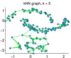
The next choice one has to make concerns the type of the graph one
wants to use, such as the -nearest neighbor or the
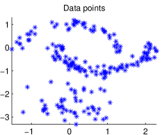
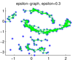
-neighborhood graph. Let us illustrate the behavior of the
different graphs using the toy example presented in Figure
3. As underlying distribution we choose a
distribution on with three clusters: two “moons” and a
Gaussian. The density of the bottom moon is chosen to be larger than
the one of the top moon. The upper left panel in Figure
3 shows a sample drawn from this
distribution. The next three panels show the different similarity
graphs on this sample.
In the -neighborhood graph, we can see that it is difficult to
choose a useful parameter . With as in the figure, the points on
the middle moon are already very tightly connected, while the points
in the Gaussian are barely connected. This problem always occurs if we
have data “on different scales”, that is the distances between data
points are different in different regions of the space.
The -nearest neighbor graph, on the other hand, can connect points
“on different scales”. We can see that points in the low-density
Gaussian are connected with points in the high-density moon. This is a
general property of -nearest neighbor graphs which can be very
useful. We can also see that the -nearest neighbor graph can break
into several disconnected components if there are high density regions
which are reasonably far away from each other. This is the case for
the two moons in this example.
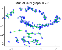
The mutual -nearest neighbor graph has the property that it tends
to connect points within regions of constant density, but does not
connect regions of different densities with each other. So the
mutual -nearest neighbor graph can be considered as being “in between”
the -neighborhood graph and the -nearest neighbor graph.
It is able to act on different scales, but does not mix those scales
with each other. Hence, the mutual -nearest neighbor graph seems
particularly well-suited if we want to detect clusters of different
densities.
The fully connected graph is very often used in connection with the
Gaussian similarity function . Here the parameter plays a
similar role as the parameter in the -neighborhood graph.
Points in local neighborhoods are connected with relatively high
weights, while edges between far away points have positive, but
negligible weights. However, the resulting similarity matrix is not a
sparse matrix.
As a general recommendation we suggest to work with the -nearest neighbor graph as the first choice. It is simple to work with, results in a sparse adjacency matrix , and in our experience is less vulnerable to unsuitable choices of parameters than the other graphs.
The parameters of the similarity graph
Once one has decided for the type of the similarity graph, one has to
choose its connectivity parameter or , respectively.
Unfortunately, barely any theoretical results are known to guide us in
this task.
In general, if the similarity graph contains more connected components
than the number of clusters we ask the algorithm to detect, then spectral
clustering will trivially return connected components as
clusters. Unless one is perfectly sure that those connected components
are the correct clusters, one should make sure that the
similarity graph is connected, or only consists of “few” connected
components and very few or no isolated vertices. There are many
theoretical results on how connectivity of random graphs can be
achieved, but all those results only hold in the limit for the sample
size . For example, it is known that for data points
drawn i.i.d. from some underlying density with a connected support
in , the -nearest neighbor graph and the mutual
-nearest neighbor graph will be connected if we choose on the
order of (e.g., ?, ?). Similar arguments
show that the parameter in the -neighborhood graph has to
be chosen as to guarantee connectivity in the limit
(?, ?).
While being of
theoretical interest, all those results do not really help us for
choosing on a finite sample.
Now let us give some rules of thumb. When working with the -nearest
neighbor graph, then the connectivity parameter should be chosen such
that the resulting graph is connected, or at least has significantly
fewer connected components than clusters we want to detect. For small or medium-sized graphs this can
be tried out ”by foot”. For very large graphs, a first approximation
could be to choose in the order of , as suggested by the
asymptotic connectivity results.
For the mutual -nearest neighbor graph, we have to admit that we
are a bit lost for rules of thumb. The advantage of the mutual
-nearest neighbor graph compared to the standard -nearest
neighbor graph is that it tends not to connect areas of different
density. While this can be good if there are clear clusters induced by
separate high-density areas, this can hurt in less obvious situations
as disconnected parts in the graph will always be chosen to be
clusters by spectral clustering. Very generally, one can observe that
the mutual -nearest neighbor graph has much fewer edges than the
standard -nearest neighbor graph for the same parameter . This
suggests to choose significantly larger for the mutual -nearest
neighbor graph than one would do for the standard -nearest neighbor
graph. However, to take advantage of the property that the
mutual -nearest neighbor graph does not connect regions of
different density, it would be necessary to allow for several “meaningful”
disconnected parts of the graph. Unfortunately, we do not know of any general
heuristic to choose the parameter such that this can be achieved.
For the -neighborhood graph, we suggest to choose such
that the resulting graph is safely connected. To determine the
smallest value of where the graph is connected is very simple:
one has to choose as the length of the longest edge in a
minimal spanning tree of the fully connected graph on the data
points. The latter can be determined easily by any minimal spanning
tree algorithm. However, note that when the data contains outliers
this heuristic will choose so large that even the outliers are
connected to the rest of the data. A similar effect happens when the
data contains several tight clusters which are very far apart from
each other. In both cases, will be chosen too large to reflect
the scale of the most important part of the data.
Finally, if one uses a fully connected graph together with a similarity
function which can be scaled itself, for example the Gaussian
similarity function, then the scale of the similarity function should
be chosen such that the resulting graph has similar properties as a
corresponding -nearest neighbor or -neighborhood graph would
have. One needs to make sure that for most data points the set of
neighbors with a similarity significantly larger than 0 is “not too
small and not too large”. In particular, for the Gaussian similarity
function several rules of thumb are frequently used. For example, one
can choose in the order of the mean distance of a point to
its -th nearest neighbor, where is chosen similarly as above
(e.g., ). Another way is to determine by the
minimal spanning tree heuristic described above, and then choose
. But note that all those rules of thumb are
very ad-hoc, and depending on the given data at hand and its
distribution of inter-point distances they might not work at all.
In general, experience shows that spectral clustering can be quite
sensitive to changes in the similarity graph and to the choice of its
parameters. Unfortunately, to our knowledge there has been no
systematic study which investigates the effects of the similarity
graph and its parameters on clustering and comes up with
well-justified rules of thumb. None of the recommendations above is
based on a firm theoretic ground. Finding rules which have a
theoretical justification should be considered an interesting and
important topic for future research.
8.2 Computing the eigenvectors
To implement spectral clustering in practice one has to compute the
first eigenvectors of a potentially large graph Laplace matrix.
Luckily, if we use the -nearest neighbor graph or the
-neighborhood graph, then all those matrices are sparse.
Efficient methods exist to compute the first eigenvectors of sparse
matrices, the most popular ones being the power method or Krylov
subspace methods such as the Lanczos method (?, ?). The
speed of convergence of those algorithms depends on the size of the
eigengap (also called spectral gap) . The larger this eigengap is, the
faster the algorithms computing the first eigenvectors converge.
Note that a general problem occurs if one of the eigenvalues under
consideration has multiplicity larger than one. For example, in the
ideal situation of disconnected clusters, the eigenvalue has
multiplicity . As we have seen, in this case the eigenspace is
spanned by the cluster indicator vectors. But unfortunately, the
vectors computed by the numerical eigensolvers do not necessarily
converge to those particular vectors. Instead they just converge to
some orthonormal basis of the eigenspace, and it usually depends on
implementation details to which basis exactly the algorithm converges.
But this is not so bad after all. Note that all vectors in the space
spanned by the cluster indicator vectors have the
form for some coefficients
, that is, they are piecewise constant on the clusters. So the
vectors returned by the eigensolvers still encode the information
about the clusters, which can then be used by the -means
algorithm to reconstruct the clusters.
8.3 The number of clusters
Choosing the number of clusters is a general problem for all
clustering algorithms, and a variety of more or less successful
methods have been devised for this problem. In model-based clustering
settings there exist well-justified criteria to choose the number of
clusters from the data. Those criteria are usually based on the
log-likelihood of the data, which can then be treated in a frequentist
or Bayesian way, for examples see ? (?). In settings where
no or few assumptions on the underlying model are made, a large
variety of different indices can be used to pick the number of
clusters. Examples range from ad-hoc measures such as the ratio of
within-cluster and between-cluster similarities, over
information-theoretic criteria (?, ?), the gap statistic
(?, ?), to stability approaches (?, ?;
?, ?; ?, ?). Of course all those
methods can also be used for spectral clustering. Additionally, one
tool which is particularly designed for spectral clustering is the
eigengap heuristic, which can be used for all three graph
Laplacians. Here the goal is to choose the number such that all
eigenvalues are very small, but
is relatively large.
There are several justifications for this procedure. The first one is
based on perturbation theory, where we observe that in the ideal case
of completely disconnected clusters, the eigenvalue has
multiplicity , and then there is a gap to the th eigenvalue
. Other explanations can be given by spectral
graph theory. Here, many geometric invariants of the graph can be
expressed or bounded with the help of the first eigenvalues of the
graph Laplacian. In particular, the sizes of cuts are closely related
to the size of the first eigenvalues. For more details on this topic
we refer to ? (?), ? (?) and ? (?).
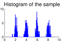
We would like to illustrate the eigengap heuristic on our toy example
introduced in Section 4. For this purpose we
consider similar data sets as in Section 4, but to
vary the difficulty of clustering we consider the Gaussians with
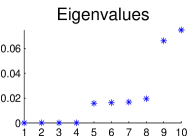
increasing variance. The first row of Figure 4
shows the histograms of the three samples. We construct the 10-nearest
neighbor graph as described in Section 4, and plot
the eigenvalues of the normalized Laplacian on
the different samples (the results for the unnormalized Laplacian are
similar). The first data set consists of four well separated clusters,
and we can see that the first 4 eigenvalues are approximately 0. Then
there is a gap between the 4th and 5th eigenvalue, that is is relatively large. According to the eigengap heuristic,
this gap indicates that the data set contains 4 clusters. The same
behavior can also be observed for the results of the fully connected
graph (already plotted in Figure 1). So we
can see that the heuristic works well if the clusters in the data are
very well pronounced.
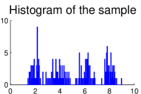
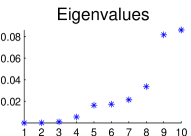
However, the more noisy or overlapping the clusters are, the less
effective is this heuristic. We can see that for the second data set
where the clusters are more “blurry”, there is still a gap between
the 4th and 5th eigenvalue, but it is not as clear to detect as in the
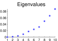
case before. Finally, in the last data set, there is no well-defined
gap, the differences between all eigenvalues are approximately the
same. But on the other hand, the clusters in this data set overlap so
much that many non-parametric algorithms will have difficulties to
detect the clusters, unless they make strong assumptions on the underlying
model. In this particular example, even for a human looking at the
histogram it is not obvious what the correct number of clusters should
be. This illustrates that, as most methods for choosing the number of
clusters, the eigengap heuristic usually works well if the data
contains very well pronounced clusters, but in ambiguous cases it also
returns ambiguous results.
Finally, note that the choice of the number of clusters and the choice of the connectivity parameters of the neighborhood graph affect each other. For example, if the connectivity parameter of the neighborhood graph is so small that the graph breaks into, say, connected components, then choosing as the number of clusters is a valid choice. However, as soon as the neighborhood graph is connected, it is not clear how the number of clusters and the connectivity parameters of the neighborhood graph interact. Both the choice of the number of clusters and the choice of the connectivity parameters of the graph are difficult problems on their own, and to our knowledge nothing non-trivial is known on their interactions.
8.4 The -means step
The three spectral clustering algorithms we presented in Section
4 use -means as last step to extract the final
partition from the real valued matrix of eigenvectors. First of all,
note that there is nothing principled about using the -means
algorithm in this step. In fact, as we have seen from the various
explanations of spectral clustering, this step should be very simple
if the data contains well-expressed clusters. For example, in the
ideal case if completely separated clusters we know that the
eigenvectors of and are piecewise constant. In this
case, all points which belong to the same cluster are
mapped to exactly the sample point , namely to the unit vector
. In such a trivial case, any clustering algorithm
applied to the points will be able to extract the correct
clusters.
While it is somewhat arbitrary what clustering algorithm exactly one
chooses in the final step of spectral clustering, one can argue that
at least the Euclidean distance between the points is a
meaningful quantity to look at. We have seen that the Euclidean
distance between the points is related to the “commute
distance” on the graph, and in ? (?) the authors show
that the Euclidean distances between the are also related to a
more general “diffusion distance”. Also, other uses of the spectral
embeddings (e.g., ? (?) or ? (?)) show
that the Euclidean distance in is meaningful.
Instead of -means, people also use other techniques to construct he
final solution from the real-valued representation. For example, in
? (?) the authors use hyperplanes for this purpose. A more
advanced post-processing of the eigenvectors is proposed in
? (?). Here the authors study the subspace spanned by
the first eigenvectors, and try to approximate this subspace as
good as possible using piecewise constant vectors. This also leads to
minimizing certain Euclidean distances in the space , which can
be done by some weighted -means algorithm.
8.5 Which graph Laplacian should be used?
A fundamental question related to spectral clustering is the question
which of the three graph Laplacians should be used to compute the
eigenvectors. Before deciding this
question, one should always look at the degree distribution of the similarity
graph. If the graph is very regular and most vertices have
approximately the same degree, then all the Laplacians are very
similar to each other, and will work equally well for clustering.
However, if the degrees in the graph are very broadly distributed, then the
Laplacians differ considerably. In our opinion, there are several
arguments which advocate for using normalized rather than unnormalized
spectral clustering, and in the normalized case to use
the eigenvectors of rather than those of .
Clustering objectives satisfied by the different algorithms
The first argument in favor of normalized spectral clustering comes from the graph partitioning point of view. For simplicity let us discuss the case . In general, clustering has two different objectives:
-
1.
We want to find a partition such that points in different clusters are dissimilar to each other, that is we want to minimize the between-cluster similarity. In the graph setting, this means to minimize .
-
2.
We want to find a partition such that points in the same cluster are similar to each other, that is we want to maximize the within-cluster similarities and .
Both and directly implement the first objective by explicitly incorporating in the objective function. However, concerning the second point, both algorithms behave differently. Note that
Hence, the within-cluster similarity is maximized if is small and if is large. As this is exactly what we achieve by minimizing , the criterion implements the second objective. This can be seen even more explicitly by considering yet another graph cut objective function, namely the criterion introduced by ? (?):
Compared to , which has the terms in the denominator, the criterion only has
in the denominator. In practice, and
are often minimized by similar cuts, as a good solution will
have a small value of anyway and hence the
denominators are not so different after all. Moreover, relaxing
leads to exactly the same optimization problem as
relaxing , namely to normalized
spectral clustering with the eigenvectors of . So one can see by several ways that normalized spectral clustering incorporates both clustering objectives mentioned above.
Now consider the case of . Here the objective is to maximize
and instead of and . But
and are not necessarily related to the within-cluster similarity, as
the within-cluster similarity depends on the edges and not on the
number of vertices in . For instance, just think of a set which has very many
vertices, all of which only have very low weighted edges to each other.
Minimizing does not attempt to maximize the
within-cluster similarity, and the same is then true for its
relaxation by
unnormalized spectral clustering.
So this is our first important point to keep in mind: Normalized
spectral clustering implements both clustering objectives mentioned
above, while unnormalized spectral clustering only implements the
first objective.
Consistency issues
A completely different argument for the superiority of normalized
spectral clustering comes from a statistical analysis of both
algorithms. In a statistical setting one assumes that the data
points have been sampled i.i.d. according to some
probability distribution on some underlying data space
. The most fundamental question is then the question of
consistency: if we draw more and more data points, do the clustering
results of spectral clustering converge to a useful partition of the
underlying space ?
For both normalized spectral clustering algorithms, it can be proved
that this is indeed the case
(?, ?, ?, ?). Mathematically,
one proves that as we take the limit , the matrix
converges in a strong sense to an operator on the space
of continuous functions on . This convergence
implies that the eigenvalues and eigenvectors of converge to
those of , which in turn can be transformed to a statement about
the convergence of normalized spectral clustering. One can show that
the partition which is induced on by the eigenvectors of
can be interpreted similar to the random walks interpretation of
spectral clustering. That is, if we consider a diffusion process on
the data space , then the partition induced by the eigenvectors
of is such that the diffusion does not transition between the
different clusters very often (?, ?). All consistency
statements about normalized spectral clustering hold, for both
and , under very mild conditions which are usually satisfied in
real world applications. Unfortunately, explaining more details about
those results goes beyond the scope of this tutorial, so we refer the
interested reader to ? (?).
In contrast to the clear convergence statements for normalized
spectral clustering, the situation for unnormalized spectral
clustering is much more unpleasant. It can be proved that
unnormalized spectral clustering can fail to converge, or that it can
converge to trivial solutions which construct clusters consisting of
one single point of the data space (?, ?, ?).
Mathematically, even though one can prove that the
matrix itself converges to some limit operator on
as , the spectral properties of this limit
operator can be so nasty that they prevent the convergence of
spectral clustering. It is possible to construct examples
which show that this is not only a problem for very large sample size,
but that it can lead to completely unreliable results even for small sample
size. At least it is possible to characterize the conditions when
those problem do not occur: We have to make sure that the eigenvalues
of corresponding to the eigenvectors used in unnormalized
spectral clustering are significantly smaller than the minimal degree in the
graph. This means that if we use the first eigenvectors for
clustering, then should hold
for all . The mathematical reason for this condition is
that eigenvectors corresponding to eigenvalues larger than
approximate Dirac functions, that is they are approximately 0 in all
but one coordinate. If those eigenvectors are used for clustering,
then they separate the one vertex where the eigenvector is non-zero
from all other vertices, and we clearly do not want to construct such
a partition. Again we refer to the literature for precise statements
and proofs.
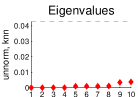
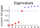
For an illustration of this phenomenon, consider again our toy data set
from Section 4. We consider the first eigenvalues
and eigenvectors of the unnormalized graph Laplacian based on the
fully connected graph, for different choices of the parameter
of the Gaussian similarity function (see last row of Figure
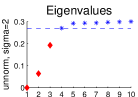
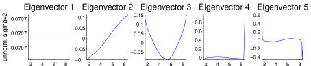
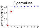
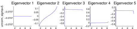
1 and all rows of Figure 5). The
eigenvalues above are plotted as blue stars, the
eigenvalues below are plotted as red diamonds. The dashed
line indicates .
In general, we can see that the eigenvectors corresponding to
eigenvalues which are much below the dashed lines are “useful”
eigenvectors. In case (plotted already in the last row of
Figure 1), Eigenvalues 2, 3 and 4 are
significantly below , and the corresponding Eigenvectors 2,
3, and 4 are meaningful (as already discussed in Section
4). If we increase the parameter , we can
observe that the eigenvalues tend to move towards . In case
, only the first three eigenvalues are below
(first row in Figure 5), and in case only
the first two eigenvalues are below (second row in Figure
5). We can see that as soon as an eigenvalue gets
close to or above , its corresponding eigenvector
approximates a Dirac function. Of course, those eigenvectors are
unsuitable for constructing a clustering. In the limit for , those eigenvectors would converge to perfect Dirac
functions. Our illustration of the finite sample case shows that this
behavior not only occurs for large sample size, but can be generated
even on the small example in our toy data set.
It is very important to stress that those problems only concern the
eigenvectors of the matrix , and they do not occur for or
. Thus, from a statistical point of view, it is preferable to
avoid unnormalized spectral clustering and to use the normalized
algorithms instead.
Which normalized Laplacian?
Looking at the differences between the two normalized spectral
clustering algorithms using and , all three explanations
of spectral clustering are in favor of . The reason is that the
eigenvectors of are cluster indicator vectors ,
while the eigenvectors of are additionally multiplied with
, which might lead to undesired artifacts. As using also
does not have any computational advantages, we thus advocate for using
.
9 Outlook and further reading
Spectral clustering goes back to ? (?), who first suggested
to construct graph partitions based on eigenvectors of the adjacency
matrix. In the same year, ? (?) discovered that
bi-partitions of a graph are closely connected with the second
eigenvector of the graph Laplacian, and he suggested to use this
eigenvector to partition a graph. Since then, spectral clustering has
been discovered, re-discovered, and extended many times in different
communities, see for example
? (?),
? (?),
? (?),
? (?), ? (?), ? (?), ? (?),
? (?),
? (?).
A nice overview over the history of spectral clustering can be found
in ? (?).
In the machine learning community, spectral clustering has been made popular
by the works of ? (?),
? (?),
? (?), and ? (?). Subsequently, spectral clustering has been extended to many non-standard settings, for example
spectral clustering applied to the co-clustering problem
(?, ?),
spectral clustering with additional side information (?, ?)
connections between spectral clustering and the weighted kernel--means
algorithm (?, ?),
learning similarity functions based on spectral clustering
(?, ?),
or spectral clustering in a distributed environment
(?, ?).
Also, new theoretical insights about the relation of spectral
clustering to other algorithms have been found. A link between
spectral clustering and the weighted kernel -means algorithm is
described in ? (?). Relations between spectral clustering
and (kernel) principal component analysis rely on the fact that the
smallest eigenvectors of graph Laplacians can also be interpreted as
the largest eigenvectors of kernel matrices (Gram matrices). Two
different flavors of this interpretation exist: while
? (?)
interpret the matrix as
kernel matrix, other authors (?, ?) interpret the
Moore-Penrose inverses of or as kernel matrix. Both
interpretations can be used to construct (different) out-of-sample
extensions for spectral clustering. Concerning application cases of
spectral clustering, in the last few years such a huge number of
papers has been published in various scientific areas that it is
impossible to cite all of them. We encourage the reader to query his
favorite literature data base with the phrase “spectral clustering”
to get an impression no the variety of applications.
The success of spectral clustering is mainly based on the fact that it
does not make strong assumptions on the form of the clusters. As
opposed to -means, where the resulting clusters form convex
sets (or, to be precise, lie in disjoint convex sets of the underlying space), spectral
clustering can solve very general problems like intertwined
spirals. Moreover, spectral clustering can be implemented efficiently
even for large data sets, as long as we make sure that the similarity
graph is sparse. Once the similarity graph is chosen, we just have to
solve a linear problem, and there are no issues of getting stuck in
local minima or restarting the algorithm for several times with
different initializations. However, we have already mentioned that
choosing a good similarity graph is not trivial, and spectral
clustering can be quite unstable under different choices of the
parameters for the neighborhood graphs.
So spectral clustering cannot serve as a “black box algorithm” which
automatically detects the correct clusters in any given data set. But
it can be considered as a powerful tool which can produce
good results if applied with care.
In the field of machine learning, graph Laplacians are not only used
for clustering, but also emerge for many other tasks such as
semi-supervised learning (e.g., ?, ? for an overview)
or manifold reconstruction (e.g., ?, ?). In most
applications, graph Laplacians are used to encode the assumption that
data points which are “close” (i.e., is large) should have
a “similar” label (i.e., ). A function
satisfies this assumption if is small for all
, that is is small. With this intuition one can use
the quadratic form as a regularizer in a transductive
classification problem. One other way to interpret the use of graph
Laplacians is by the smoothness assumptions they encode. A function
which has a low value of has the property that it
varies only “a little bit” in regions where the data points lie
dense (i.e., the graph is tightly connected), whereas it is allowed to
vary more (e.g., to change the sign) in regions of low data density.
In this sense, a small value of encodes the so called
“cluster assumption” in semi-supervised learning, which requests
that the decision boundary of a
classifier should lie in a region of low density.
An intuition often used is that graph Laplacians formally look like a continuous Laplace operator (and this is also where the name “graph Laplacian” comes from). To see this, transform a local similarity to a distance by the relationship and observe that
looks like a difference quotient. As a consequence, the equation from Proposition 1 looks like a discrete version of the quadratic form associated to the standard Laplace operator on , which satisfies
This intuition has been made precise in the works of ? (?), ? (?),
? (?, ?), ? (?), ? (?),
? (?).
In general, it is proved that graph Laplacians are
discrete versions of certain continuous Laplace operators, and that if
the graph Laplacian is constructed on a similarity graph of randomly
sampled data points, then it converges to some continuous Laplace
operator (or Laplace-Beltrami operator) on the underlying space.
? (?) studied the first important step of the convergence
proof, which deals with the convergence of a continuous operator
related to discrete graph Laplacians to the Laplace-Beltrami
operator. His results were generalized from uniform distributions to general
distributions by ? (?). Then in ? (?), the
authors prove pointwise convergence results for the unnormalized graph
Laplacian using the Gaussian similarity function on manifolds with
uniform distribution. At the same time, ? (?) prove more
general results, taking into account all different graph Laplacians
, , and , more general similarity functions, and
manifolds with arbitrary distributions. In ? (?),
distributional and uniform convergence results are proved on manifolds
with uniform distribution. ? (?) studies the convergence of
the smoothness functional induced by the graph
Laplacians and shows uniform convergence results.
Apart from applications of graph Laplacians to partitioning problems in the widest sense, graph Laplacians can also be used for completely different purposes, for example for graph drawing (?, ?). In fact, there are many more tight connections between the topology and properties of graphs and the graph Laplacian matrices than we have mentioned in this tutorial. Now equipped with an understanding for the most basic properties, the interested reader is invited to further explore and enjoy the huge literature in this field on his own.
References
- Aldous FillAldous Fill Aldous, D. Fill, J. (in preparation). Reversible Markov Chains and Random Walks on Graphs. online version available at http://www.stat.berkeley.edu/users/aldous/RWG/book.html.
- Bach JordanBach Jordan Bach, F. Jordan, M. (2004). Learning spectral clustering. In S. Thrun, L. Saul, B. Schölkopf (Eds.), Advances in Neural Information Processing Systems 16 (NIPS) (pp. 305 – 312). Cambridge, MA: MIT Press.
- Bapat, Gutman, XiaoBapat et al. Bapat, R., Gutman, I., Xiao, W. (2003). A simple method for computing resistance distance. Z. Naturforsch., 58, 494 – 498.
- Barnard, Pothen, SimonBarnard et al. Barnard, S., Pothen, A., Simon, H. (1995). A spectral algorithm for envelope reduction of sparse matrices. Numerical Linear Algebra with Applications, 2(4), 317 – 334.
- BelkinBelkin Belkin, M. (2003). Problems of Learning on Manifolds. PhD Thesis, University of Chicago.
- Belkin NiyogiBelkin Niyogi Belkin, M. Niyogi, P. (2003). Laplacian eigenmaps for dimensionality reduction and data representation. Neural Computation, 15(6), 1373 – 1396.
- Belkin NiyogiBelkin Niyogi Belkin, M. Niyogi, P. (2005). Towards a theoretical foundation for Laplacian-based manifold methods. In P. Auer R. Meir (Eds.), Proceedings of the 18th Annual Conference on Learning Theory (COLT) (pp. 486 – 500). Springer, New York.
- Ben-David, von Luxburg, PálBen-David et al. Ben-David, S., von Luxburg, U., Pál, D. (2006). A sober look on clustering stability. In G. Lugosi H. Simon (Eds.), Proceedings of the 19th Annual Conference on Learning Theory (COLT) (pp. 5 – 19). Springer, Berlin.
- Bengio et al.Bengio et al. Bengio, Y., Delalleau, O., Roux, N., Paiement, J., Vincent, P., Ouimet, M. (2004). Learning eigenfunctions links spectral embedding and kernel PCA. Neural Computation, 16, 2197 – 2219.
- Ben-Hur, Elisseeff, GuyonBen-Hur et al. Ben-Hur, A., Elisseeff, A., Guyon, I. (2002). A stability based method for discovering structure in clustered data. In Pacific Symposium on Biocomputing (pp. 6 – 17).
- BhatiaBhatia Bhatia, R. (1997). Matrix Analysis. Springer, New York.
- Bie CristianiniBie Cristianini Bie, T. D. Cristianini, N. (2006). Fast SDP relaxations of graph cut clustering, transduction, and other combinatorial problems . JMLR, 7, 1409 – 1436.
- BollaBolla Bolla, M. (1991). Relations between spectral and classification properties of multigraphs (Technical Report No. DIMACS-91-27). Center for Discrete Mathematics and Theoretical Computer Science.
- BrémaudBrémaud Brémaud, P. (1999). Markov chains: Gibbs fields, Monte Carlo simulation, and queues. New York: Springer-Verlag.
- Brito, Chavez, Quiroz, YukichBrito et al. Brito, M., Chavez, E., Quiroz, A., Yukich, J. (1997). Connectivity of the mutual k-nearest-neighbor graph in clustering and outlier detection. Statistics and Probability Letters, 35, 33 – 42.
- Bui JonesBui Jones Bui, T. N. Jones, C. (1992). Finding good approximate vertex and edge partitions is NP-hard. Inf. Process. Lett., 42(3), 153 – 159.
- Chapelle, Schölkopf, ZienChapelle et al. Chapelle, O., Schölkopf, B., Zien, A. (Eds.). (2006). Semi-Supervised Learning. MIT Press, Cambridge.
- ChungChung Chung, F. (1997). Spectral graph theory (Vol. 92 of the CBMS Regional Conference Series in Mathematics). Conference Board of the Mathematical Sciences, Washington.
- DhillonDhillon Dhillon, I. (2001). Co-clustering documents and words using bipartite spectral graph partitioning. In Proceedings of the seventh ACM SIGKDD international conference on Knowledge discovery and data mining (KDD) (pp. 269 – 274). New York: ACM Press.
- Dhillon, Guan, KulisDhillon et al. Dhillon, I., Guan, Y., Kulis, B. (2005). A unified view of kernel -means, spectral clustering, and graph partitioning (Technical Report No. UTCS TR-04-25). University of Texas at Austin.
- DingDing Ding, C. (2004). A tutorial on spectral clustering. Talk presented at ICML. (Slides available at http://crd.lbl.gov/~cding/Spectral/)
- Ding, He, Zha, Gu, SimonDing et al. Ding, C., He, X., Zha, H., Gu, M., Simon, H. (2001). A min-max cut algorithm for graph partitioning and data clustering. In Proceedings of the first IEEE International Conference on Data Mining (ICDM) (pp. 107 – 114). Washington, DC, USA: IEEE Computer Society.
- Donath HoffmanDonath Hoffman Donath, W. E. Hoffman, A. J. (1973). Lower bounds for the partitioning of graphs. IBM J. Res. Develop., 17, 420 – 425.
- FiedlerFiedler Fiedler, M. (1973). Algebraic connectivity of graphs. Czechoslovak Math. J., 23, 298 – 305.
- Fouss, Pirotte, Renders, SaerensFouss et al. Fouss, F., Pirotte, A., Renders, J.-M., Saerens, M. (2007). Random-walk computation of similarities between nodes of a graph with application to collaborative recommendation. IEEE Trans. Knowl. Data Eng, 19(3), 355–369.
- Fraley RafteryFraley Raftery Fraley, C. Raftery, A. E. (2002). Model-based clustering, discriminant analysis, and density estimation. JASA, 97, 611 – 631.
- Giné KoltchinskiiGiné Koltchinskii Giné, E. Koltchinskii, V. (2005). Empirical graph Laplacian approximation of Laplace-Beltrami operators: large sample results. In Proceedings of the 4th International Conference on High Dimensional Probability (pp. 238 – 259).
- Golub Van LoanGolub Van Loan Golub, G. Van Loan, C. (1996). Matrix computations. Baltimore: Johns Hopkins University Press.
- Guattery MillerGuattery Miller Guattery, S. Miller, G. (1998). On the quality of spectral separators. SIAM Journal of Matrix Anal. Appl., 19(3), 701 – 719.
- Gutman XiaoGutman Xiao Gutman, I. Xiao, W. (2004). Generalized inverse of the Laplacian matrix and some applications. Bulletin de l’Academie Serbe des Sciences at des Arts (Cl. Math. Natur.), 129, 15 – 23.
- Hagen KahngHagen Kahng Hagen, L. Kahng, A. (1992). New spectral methods for ratio cut partitioning and clustering. IEEE Trans. Computer-Aided Design, 11(9), 1074 – 1085.
- Hastie, Tibshirani, FriedmanHastie et al. Hastie, T., Tibshirani, R., Friedman, J. (2001). The elements of statistical learning. New York: Springer.
- HeinHein Hein, M. (2006). Uniform convergence of adaptive graph-based regularization. In Proceedings of the 19th Annual Conference on Learning Theory (COLT) (pp. 50 – 64). Springer, New York.
- Hein, Audibert, von LuxburgHein et al. Hein, M., Audibert, J.-Y., von Luxburg, U. (2005). From graphs to manifolds - weak and strong pointwise consistency of graph Laplacians. In P. Auer R. Meir (Eds.), Proceedings of the 18th Annual Conference on Learning Theory (COLT) (pp. 470 – 485). Springer, New York.
- Hendrickson LelandHendrickson Leland Hendrickson, B. Leland, R. (1995). An improved spectral graph partitioning algorithm for mapping parallel computations. SIAM J. on Scientific Computing, 16, 452 – 469.
- JoachimsJoachims Joachims, T. (2003). Transductive Learning via Spectral Graph Partitioning. In T. Fawcett N. Mishra (Eds.), Proceedings of the 20th international conference on machine learning (ICML) (pp. 290 – 297). AAAI Press.
- Kannan, Vempala, VettaKannan et al. Kannan, R., Vempala, S., Vetta, A. (2004). On clusterings: Good, bad and spectral. Journal of the ACM, 51(3), 497–515.
- Kempe McSherryKempe McSherry Kempe, D. McSherry, F. (2004). A decentralized algorithm for spectral analysis. In Proceedings of the 36th Annual ACM Symposium on Theory of Computing (STOC) (pp. 561 – 568). New York, NY, USA: ACM Press.
- Klein RandicKlein Randic Klein, D. Randic, M. (1993). Resistance distance. Journal of Mathematical Chemistry, 12, 81 – 95.
- KorenKoren Koren, Y. (2005). Drawing graphs by eigenvectors: theory and practice. Computers and Mathematics with Applications, 49, 1867 – 1888.
- LafonLafon Lafon, S. (2004). Diffusion maps and geometric harmonics. PhD Thesis, Yale University.
- LangLang Lang, K. (2006). Fixing two weaknesses of the spectral method. In Y. Weiss, B. Schölkopf, J. Platt (Eds.), Advances in Neural Information Processing Systems 18 (pp. 715 – 722). Cambridge, MA: MIT Press.
- Lange, Roth, Braun, BuhmannLange et al. Lange, T., Roth, V., Braun, M., Buhmann, J. (2004). Stability-based validation of clustering solutions. Neural Computation, 16(6), 1299 – 1323.
- LovászLovász Lovász, L. (1993). Random walks on graphs: a survey. In Combinatorics, Paul Erdös is eighty (pp. 353 – 397). Budapest: János Bolyai Math. Soc.
- LütkepohlLütkepohl Lütkepohl, H. (1997). Handbook of Matrices. Chichester: Wiley.
- M., Audibert, von LuxburgM. et al. M., Audibert, J.-Y., von Luxburg, U. (2007). Graph laplacians and their convergence on random neighborhood graphs. JMLR, 8, 1325 – 1370.
- Meila ShiMeila Shi Meila, M. Shi, J. (2001). A random walks view of spectral segmentation. In 8th International Workshop on Artificial Intelligence and Statistics (AISTATS).
- MoharMohar Mohar, B. (1991). The Laplacian spectrum of graphs. In Graph theory, combinatorics, and applications. Vol. 2 (Kalamazoo, MI, 1988) (pp. 871 – 898). New York: Wiley.
- MoharMohar Mohar, B. (1997). Some applications of Laplace eigenvalues of graphs. In G. Hahn G. Sabidussi (Eds.), Graph Symmetry: Algebraic Methods and Applications (Vol. NATO ASI Ser. C 497, pp. 225 – 275). Kluwer.
- Nadler, Lafon, Coifman, KevrekidisNadler et al. Nadler, B., Lafon, S., Coifman, R., Kevrekidis, I. (2006). Diffusion maps, spectral clustering and eigenfunctions of Fokker-Planck operators. In Y. Weiss, B. Schölkopf, J. Platt (Eds.), Advances in Neural Information Processing Systems 18 (pp. 955 – 962). Cambridge, MA: MIT Press.
- Ng, Jordan, WeissNg et al. Ng, A., Jordan, M., Weiss, Y. (2002). On spectral clustering: analysis and an algorithm. In T. Dietterich, S. Becker, Z. Ghahramani (Eds.), Advances in Neural Information Processing Systems 14 (pp. 849 – 856). MIT Press.
- NorrisNorris Norris, J. (1997). Markov Chains. Cambridge: Cambridge University Press.
- PenrosePenrose Penrose, M. (1999). A strong law for the longest edge of the minimal spanning tree. Ann. of Prob., 27(1), 246 – 260.
- Pothen, Simon, LiouPothen et al. Pothen, A., Simon, H. D., Liou, K. P. (1990). Partitioning sparse matrices with eigenvectors of graphs. SIAM Journal of Matrix Anal. Appl., 11, 430 – 452.
- Saerens, Fouss, Yen, DupontSaerens et al. Saerens, M., Fouss, F., Yen, L., Dupont, P. (2004). The principal components analysis of a graph, and its relationships to spectral clustering. In Proceedings of the 15th European Conference on Machine Learning (ECML) (pp. 371 – 383). Springer, Berlin.
- Shi MalikShi Malik Shi, J. Malik, J. (2000). Normalized cuts and image segmentation. IEEE Transactions on Pattern Analysis and Machine Intelligence, 22(8), 888 – 905.
- SimonSimon Simon, H. (1991). Partitioning of unstructured problems for parallel processing. Computing Systems Engineering, 2, 135 – 148.
- Spielman TengSpielman Teng Spielman, D. Teng, S. (1996). Spectral partitioning works: planar graphs and finite element meshes. In 37th Annual Symposium on Foundations of Computer Science (Burlington, VT, 1996) (pp. 96 – 105). Los Alamitos, CA: IEEE Comput. Soc. Press. (See also extended technical report.)
- Stewart SunStewart Sun Stewart, G. Sun, J. (1990). Matrix Perturbation Theory. New York: Academic Press.
- Still BialekStill Bialek Still, S. Bialek, W. (2004). How many clusters? an information-theoretic perspective. Neural Comput., 16(12), 2483 – 2506.
- Stoer WagnerStoer Wagner Stoer, M. Wagner, F. (1997). A simple min-cut algorithm. J. ACM, 44(4), 585 – 591.
- Tibshirani, Walther, HastieTibshirani et al. Tibshirani, R., Walther, G., Hastie, T. (2001). Estimating the number of clusters in a dataset via the gap statistic. J. Royal. Statist. Soc. B, 63(2), 411 – 423.
- Van Driessche RooseVan Driessche Roose Van Driessche, R. Roose, D. (1995). An improved spectral bisection algorithm and its application to dynamic load balancing. Parallel Comput., 21(1), 29 – 48.
- von Luxburg, Belkin, Bousquetvon Luxburg et al. von Luxburg, U., Belkin, M., Bousquet, O. (to appear). Consistency of spectral clustering. Annals of Statistics. (See also Technical Report 134, Max Planck Institute for Biological Cybernetics, 2004)
- von Luxburg, Bousquet, Belkinvon Luxburg et al. von Luxburg, U., Bousquet, O., Belkin, M. (2004). On the convergence of spectral clustering on random samples: the normalized case. In J. Shawe-Taylor Y. Singer (Eds.), Proceedings of the 17th Annual Conference on Learning Theory (COLT) (pp. 457 – 471). Springer, New York.
- von Luxburg, Bousquet, Belkinvon Luxburg et al. von Luxburg, U., Bousquet, O., Belkin, M. (2005). Limits of spectral clustering. In L. Saul, Y. Weiss, L. Bottou (Eds.), Advances in Neural Information Processing Systems (NIPS) 17 (pp. 857 – 864). Cambridge, MA: MIT Press.
- Wagner WagnerWagner Wagner Wagner, D. Wagner, F. (1993). Between min cut and graph bisection. In Proceedings of the 18th International Symposium on Mathematical Foundations of Computer Science (MFCS) (pp. 744 – 750). London: Springer.