The Abdus Salam International Centre for Theoretical Physics, Strada Costiera 11, 34014 Trieste, Italy
Relative population size, co-operation pressure and strategy correlation in two-population evolutionary dynamics
Abstract
We study the coupled dynamics of two populations of random replicators by means of statistical mechanics methods, and focus on the effects of relative population size, strategy correlations and heterogeneities in the respective co-operation pressures. To this end we generalise existing path-integral approaches to replicator systems with random asymmetric couplings. This technique allows one to formulate an effective dynamical theory, which is exact in the thermodynamic limit and which can be solve for persistent order parameters in a fixed-point regime regardless of the symmetry of the interactions. The onset of instability can be determined self-consistently. We calculate quantities such as the diversity of the respective populations and their fitnesses in the stationary state, and compare results with data from a numerical integration of the replicator equations.
pacs:
02.50.Le, 75.10.Nr, 87.23.Kg1 Introduction
The evolutionary dynamics of populations of interacting species is often described by so-called replicator equations (RE) Book4 ; Book5 . Each species here carries a fitness, and species who are fitter than the average increase in concentration whereas the weight of species less fit than average decreases. RE have also found applications in game theory and economics Book6 , and an equivalence to Lotka-Volterra equations of population dynamics can be established. In the context of game theory RE describe situations in which a game is played repeatedly by players chosen randomly from populations of agents. Each individual agent here plays one fixed (so-called pure) strategy throughout his lifetime, and reproduction occurs in proportion to the payoff accrued. Offspring then inherit the strategy of their parent. In this situation the replicators are hence the pure strategies of the game under consideration. In this paper we will use the interpretations of RE in population dynamics and in evolutionary game theory simultaneously, and will hence refer to the replicating entities as ‘species’ and ‘strategies’ synonymously. Similarly, ‘fitness’ and ‘payoff’ will be used interchangeably.
The analysis of eco-systems and replicators with fixed random couplings was initiated by the seminal work of May , and although the study of real-world eco-systems has since then moved on the incorporate more realistic and evolving networks (see e.g. McKane_Drossel_2005 and references therein), replicator systems with quenched random couplings are still of interest from the statistical mechanics perspective and as an analytically tractable benchmark. Techniques from disordered systems theory have first been applied to such models in DO ; OD ; OD2 ; ParisiBiscari and focus both on static approaches based on the replica method and on dynamical studies by means of generating functional techniques. The latter approach here has the advantage of being able to address couplings of general symmetry OD ; galla , whereas replica theory is restricted to cases of symmetric interaction (see OF1 ; OF2 ; OF3 ; OL ; SF ; Tokita for further replica studies of random replicator models). In the course of these studies complex non-trivial behaviour of random replicator systems has been identified, with several types of phase transitions between stable and unstable regimes, and multiple patterns of ergodicity breaking. While most of the existing studies have focused on so-called single-population models, corresponding to games with only one type of player, multi-population models have recently been addressed in epl , where a relation between the stability of two-population replicator systems and the corresponding two-player bi-matrix games has been considered. These are games in which the two interacting players take different roles (e.g. female versus male), and may hence have different sets of strategies at their disposal (as opposed to single-population games such as rock-papers-scissors, where the strategy pool is identical for both players). Static studies of random matrix games can also be found in berg ; berg2 ; berg3 .
The aim of the present work is to extend the studies of epl to the case of two interacting populations of different relative size and to incorporate correlations between payoff matrices as well as heterogeneity in the co-operation pressures of species. We first present the details of the model in the next section, and then formulate an effective macroscopic theory in the thermodynamic limit. Specific results are then reported in section 4, where we test the predictions of the resulting fixed-point theory against numerical simulations. A summary and outlook conclude the paper.
2 Model
We consider two populations of replicators (abbreviated as and in the following), where we denote the species in system by , and the ones in population by . and are hence the sizes of the two populations (equivalently the number of pure strategies available to the two types of players of the bi-matrix game). We will consider the general case , and will write and in the following. The statistical mechanics analysis is then concerned with the limit , where the ratios and remain finite. The aspect ratio is hence a control parameter of the model.
We will refer to the species in as species of type , and to species in as species of type . The composition of at time is then characterised by a concentration vector , where indicates the relative weight of species in . Similarly, the configuration of can be described by . In the context of evolutionary game theory, vectors of this type characterise mixed strategies Book6 , with e.g. being proportional to the probability of a player of type using pure strategy . We will in the following use the normalisation and , which will allow us to formulate a well-defined thermodynamic limit of the problem.
Species of type are assumed to interact only with species of type and vice versa, and the populations are taken to follow the following replicator equations
| (1) |
and are here the co-operation pressures acting on the two populations. Depending on their strengths and limit the growth of individual species and drive and towards states with many surviving species and high diversity Book5 . We will mostly consider the situation in which . The payoff matrices (or inter-species couplings) are drawn from a Gaussian distribution with the following first two moments:
| (2) |
The overbar denotes an average over the disorder, i.e. over samples of the random payoff matrices. All other covariances are taken to vanish. The scaling of the covariance matrix with the system size is here again chosen to guarantee a well-defined thermodynamic limit , with which the statistical mechanics theory will be concerned. is a model parameter, characterising the symmetry or otherwise of the interaction: for we have corresponding to prey-predator relations in population dynamics, and to a zero-sum game in the context of evolutionary game theory. For and are uncorrelated, while corresponds to the case of symmetric interaction, . Intermediate values of allow for a smooth interpolation between these cases. and finally are the time-dependent mean fitnesses of species in the two respective populations,
| (3) |
where denotes the fitness of species (the superscript indicates that this species belongs to ). is defined similarly. These definitions ensure that the replicator equations (1) conserve the normalisations in time. Initial conditions in our simulations are chosen to respect this normalisation.
3 Statistical mechanics theory
3.1 Uncorrelated strategies
The dynamics of the model can be reduced to two coupled stochastic processes for a representative pair of ‘effective’ species, one from each population. We will not detail the mathematical steps here, but will only quote the final outcome. Similar calculations can be found in OD ; galla or, in a different context, in the textbook Book2 . The generating functional analysis delivers the following effective dynamics:
where and represent coloured Gaussian noise of zero mean and with covariances to be determined self-consistently as
| (5) |
here refers to an average over realisations of the effective processes, i.e. over paths of . The response functions and , in turn, are given by
| (6) |
respectively. As usual in the dynamics of disordered systems these processes are non-Markovian (as reflected by the retarded interaction terms), and the resulting single-particle noises exhibit non-trivial temporal correlations. The description in terms of the above effective processes is equivalent to the original problem in the thermodynamic limit in the sense that combined disorder-species-averages in the microscopic problem can be evaluated as averages over realisations of the effective single-particle noise (see Book2 for further technical details regarding the generating functional technique).
Following OD , we proceed with a fixed-point analysis of (LABEL:eq:effproc), based on the assumption of time-translation invariance and finite integrated responses
| (7) |
(). We also write and , where and denote the fixed point values of the single-species concentrations obtained from (LABEL:eq:effproc) as . Since each realisation of the single-species trajectories is a time-dependent stochastic process, the resulting fixed point values and are static random variables. See OD ; galla for further technical details regarding this approach.
The fixed-point ansatz then leads to the following six equations for the persistent order parameters
:
| (8) |
where and and where for . These equations are readily solved to yield the persistent order parameters as functions of the model parameters . It is here efficient to proceed as proposed in SF and to obtain parametric solutions in terms of , i.e. to fix the values of these two quantities, and then to obtain from the left-hand sides of (8). Note that and are the fractions of surviving species, in the two respective populations. In the context of game theory these expressions correspond to the fractions of pure strategies played with non-zero probabilities berg ; berg2 ; berg3 . As seen in galla and serve as measures of the resulting diversities as well. is here given by at the fixed point, and a similar definition of applies. If e.g. all species are present at equal concentration in (, then . If however only a few species survive in , then (in the extreme case of only one species surviving, say and for one has which tends to infinity in the thermodynamic limit). A detailed inspection shows that and are closely related to what is referred to Simpson’s index of diversity in ecology simpson .
3.2 Correlated strategies
We will below also consider the case of correlated strategies as proposed in berg ; berg2 . Here, the moments of the matrix elements are further constrained by imposing
| (9) |
with correlation parameters . We will furthermore restrict the analysis to the case when considering strategy correlations, we then have . and measure the correlations within rows and columns of the payoff matrix. I.e. if is large, the elements
bear some correlation for any fixed , reflecting a reduction of the variability of strategies in (all pure strategies in bear some degree of similarity). Similarly, an increased value of makes pure strategies in more alike, and hence reduces the strategic options of individuals in that population.
These strategy correlations can be incorporated in the path-integral analysis, and lead to the following modifications in the resulting effective processes:
The covariances of the effective single-species noises are now given by
| (11) |
and as before. The resulting equations for the persistent order parameters undergo the corresponding changes as well (we do not report them here).
3.3 Stability
The stability of the fixed point identified and used in the above ansatz can be investigated by means of a linear expansion about the assumed fixed point values of the concentrations of the effective pure strategy frequencies and and of the stationary noise variables and . We will not go into details here, as the analysis follows the lines of OD . The final outcome is that the system is stable whenever
| (12) |
and that non-trivial and non-decaying fluctuations may arise whenever this condition is violated, so that the above fixed-point ansatz breaks down and Eqs. (8) can no longer be expected to describe the behaviour of the model accurately. For the above condition reduces to the one reported in epl . We also remark that, if additionally , Eqs. (8) reduce to the one-population results of OD ; galla . The onset of instability then occurs at , as first reported in OD .
4 Results
4.1 Populations with different co-operation pressures
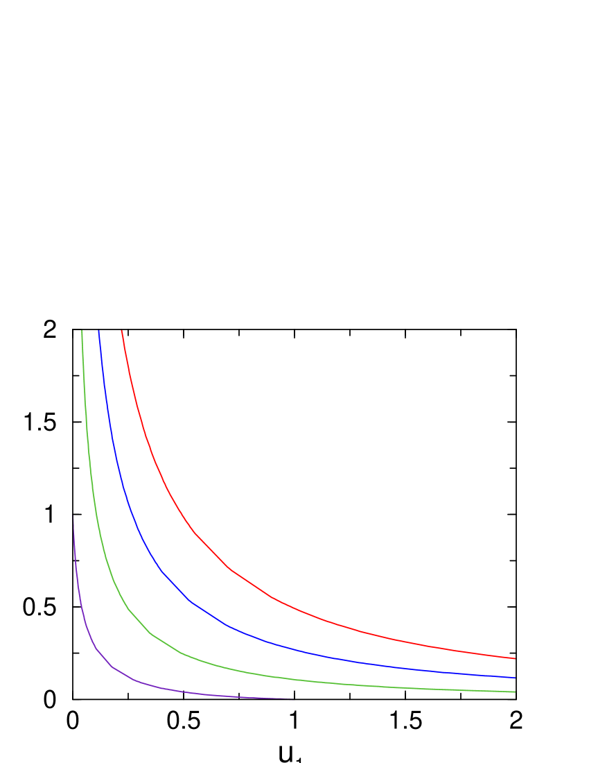
We first study the case of equally large populations, , and focus on the effects of the co-operation pressures and on the stability and behaviour of the system. The resulting phase diagram has been reported in epl , and is re-iterated in Fig. 1 for completeness. The replicator dynamics, for any given realisation of the coupling matrices, evolve into a unique stable fixed point at large co-operation pressure. Below the phase transition lines depicted in Fig. 1, the system becomes non-ergodic in the sense that multiple microscopic stationary states exists, and initial conditions determine which of these is assumed asymptotically. For fully symmetric couplings the system still evolves into a fixed point, but exponentially many (in ) fixed points can be expected to exist DO ; OD ; OD2 . For , i.e. for systems with partially or fully uncorrelated or anti-correlated couplings, no such behaviour is observed, and the dynamics may evolve towards a volatile, potentially chaotic state.
The role of the two co-operation pressures is to drive the respective populations into the internal region of their concentration simplices (defined by the constraints
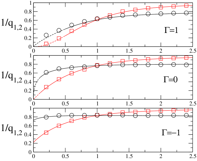
and ). Hence co-operation pressure promotes the survival of many pure strategies, or in other words a diverse stationary state. In order to study the effects of and we report results for a fixed value in Fig. 2 and depict results for the diversity parameters and of the respective populations, as is varied. As expected both diversities are increasing functions of . The effect on population is here much more direct, but remarkably, for small values of the diversity of population is a steep function of as well, at least for symmetric and asymmetric couplings. This indicates a feedback from population onto population : decreasing the co-operation pressure on population leads to depletion in this population and this may then impact on the diversity of the other population as well, even though is kept constant.
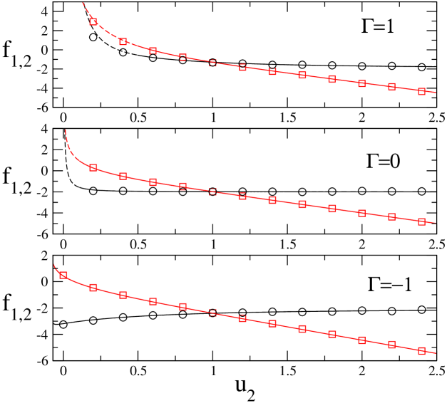
In Figs. 3 and 4 we report on the fitness of the two populations. One here has to distinguish between the contributions of co-operation pressure and of the direct interaction to the overall fitness. While the Lagrange parameters entail the effects of co-operation pressures as well, we study the fitnesses and purely due to direct interaction in Fig. 4. As shown in Fig. 3 an increase of typically reduces and , provided , i.e. provided that there is no degree of anti-correlation present in the coupling matrices. Again the effects of a change in are much more pronounced in than in , and remains almost constant except for a region at small values of . For negative values of the effect is quite different, as seen in the lower panel of Fig. 3. While, as before, is a decreasing function of , non-trivial behaviour is induced in population , and is found to be increasing in , especially when small. This is the regime in which strongly controls the diversity of population , and a reduction of the diversity in appears to impact negatively on the fitness of .
In order to disentangle the effects of co-operation pressure related contributions to the fitnesses, we study the behaviour of , in Fig. 4. For positive strategy correlation, we find that both fitnesses decrease as in increased. The non-trivial behaviour at negative strategy correlation remains, however, and is found to be a non-monotonous function of , again signalling an indirect impact of the diversity of on the payoff of .
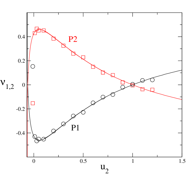
An interesting effect is observed for the case , i.e. for full anti-correlation, see Fig. 5. In order to characterise the behaviour of , we have here extended the range of the co-operation pressures to include small negative values of . In the zero-sum case one has by construction, and both fitnesses are found to be non-monotonic functions of at fixed co-operation pressure in population . In particular a maximum of the fitness of is found as the co-operation pressure is increased, whereas the other population experiences a minimum in fitness under these conditions.111We here remark that while numerical experiments agree near perfectly with the theoretical predictions for positive , they become less reliable at , where the theoretical curves are fairly steep. The accuracy of simulations might here suffer from a small number of surviving species and the associated finite-size effects and sample-to-sample fluctuations.
4.2 Effects of relative population size
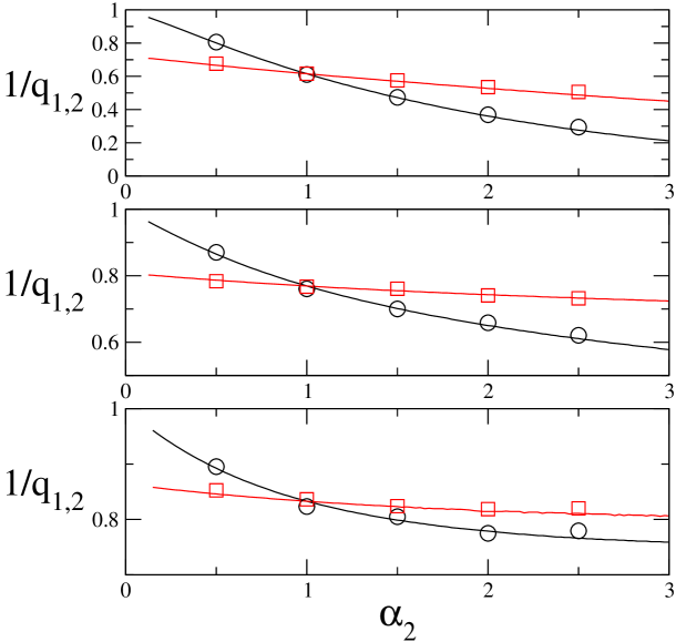
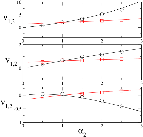
The effects of varying the relative system size of the two populations are illustrated in Figs. 6 and 7. We here first follow berg ; berg2 and fix the size parameter in the first population, and vary the size of . As shown in Fig. 6, the diversities of both populations decrease as is increased. The effect is much stronger in than in . In Fig. 7 we depict the fitnesses of the the two populations for this case of rectangular payoff matrices . We find that, within our settings and for , both populations profit from reducing the aspect ratio , where the increase of fitness appears more pronounced for than for . Thus it appears it is the size of the population with which a given species interacts, rather than the size of its own population, which determines the fitness of this given species. Inspection of the case of full anti-correlation (lower panel in Fig. 7) shows that the fitness of may display non-monotonic behaviour as a function of . We note here that for the case of fully symmetric couplings (), and that for , i.e. for . These relations are due to the construction of the model, where one has and as well as . No such simple relations between the resulting are found for , as and are then neither fully correlated nor fully anti-correlated.
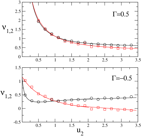
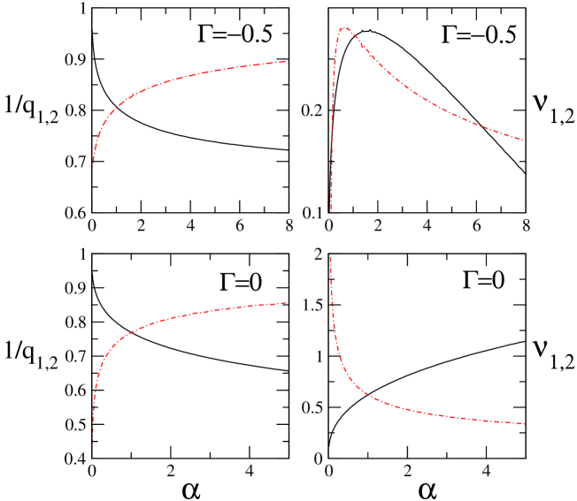
The results described so far in this section are not found to be symmetrical around , In a symmetrical situation, where only the aspect ratio matters, one would expect that choosing is equivalent to setting for any , subject to a relabelling of the two populations. Recall, however that the coupling strengths remain fixed and are given by . The respective sizes of the two populations are and , where we fixed above. These definitions follow those of berg ; berg2 . A more symmetrical setup can be achieved by setting e.g. and , with the aspect ratio . As seen in Fig. 8, the diversity of population decreases as its relative size is increases, whereas is monotonically decreasing (we do not report simulation results here to keep the figure readable). The behaviour of the fitnesses crucially depends on the symmetry of couplings, with multiple crossings of and observed for suitable model parameters as shown in Fig. 8.
4.3 Strategy correlations
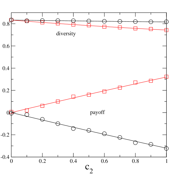
Finally, we have examined the effects of strategy correlations. We here fix and . Results are presented in Fig. 9, where we depict the case of varying at fixed . As seen in the figure, the diversity (or equivalently the fraction of pure strategies played with non-zero probability) decreases in both populations as is increased. The effect is stronger in than in . At the same time, the payoff for population two increases as the correlation parameter is increased, whereas the payoff for decreases (note that by construction, as we are considering the case of zero-sum games, ). The condensation of into a small subset of strategies can here be understood as follows: an increased value of induces correlations within the columns of the payoff matrix , so that in the extreme case of large , the become mostly independent of . Thus the payoff for both players becomes more and more independent of the action of player , and depends only on the choice of player . In other words, the strategies available to player become more and more alike as is increased, thus rendering some of ’s strategies generally beneficial for (independently of the choice of ), and others detrimental. Hence, will mostly play strategies beneficial from his perspective and will reduce the diversity of his actions, while at the same time increasing his payoff , as seen in Fig. 9. See also berg for similar cases. A more symmetrical situation can be constructed by considering , a case in which correlations are present both in the rows and columns of the payoff matrix. We do not depict results here, but only remark that in this case the diversity of both populations decreases as is increased (the payoff for both populations remains strictly zero in this case due to the zero-sum property of the games considered, and the exchange symmetry between and ).
4.4 One-population models with heterogeneous co-operation pressure
In this section we will consider a single-population replicator model with heterogeneous (i.e. species-dependent) co-operation pressures. Specifically consider species subject to the replicator equations
| (13) |
where the coupling matrix is a Gaussian random quantity as in OD (, but where the co-operation pressure now carries a species index , and where each is assumed to be drawn independently from the distribution at the beginning of the dynamics and then remains fixed. Note that while the overall concentration is conserved, species subject to a certain (e.g. high) co-operation pressure may well die out or be reduced in concentration to the advantage of species of a lesser co-operation pressure.
The further analysis leads to an ensemble of effective processes, one for each value of in the support of :
The response function is now defined as
. Furthermore we have independently of . A fixed point ansatz results in the following self-consistent equations for the integrated response , the (inverse) diversity parameter and the fitness :
| (15) |
where . While we note that the fitnesses of any surviving species come out as equal (and independent of their co-operation pressures), their relative concentrations
| (16) |
and second moments
| (17) |
(suitable sample-averages are implied) maybe well be dependent on 222We here note that the fraction of survivors (with the step function) comes out as independent of , and is given by .. Here denotes the set of species with co-operation pressure , with an infinitesimal element. Overall self-consistency requires that and .
We will here restrict to the case of a flat distribution over the interval , so that the integrals on the right-hand side of (15) can be performed explicitly to give
| (18) |
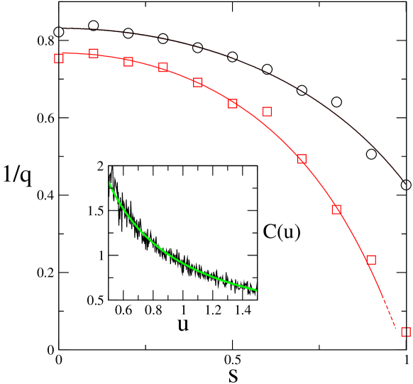
Results are shown and compared with simulations in Fig. 10. Interestingly one observes a decline in diversity of the population as the variability of the co-operation pressure is increased. Thus increasing the complexity of the properties of the individual species might lead to a less diverse composition of the eco-system at stationarity. This effect seems to be mostly independent of the symmetry of the couplings333We have not been able to solve the resulting fixed-point equations for at large widths of the distribution of co-operation pressures.. The inset of Fig. 10 demonstrates that the relative weight of species subject to co-operation decreases non-linearly with , so that species with comparably low co-operation pressure dominate the population at the fixed point. More precisely is found to be given by , i.e. it roughly decays as the inverse power of . As seen in the inset of the figure the theoretical prediction of this behaviour agrees perfectly with results from simulations.
5 Conclusions
In summary, we have extended existing generating functional techniques to study the behaviour of two-population replicator systems, and have focused on the effects of co-operation pressure, relative population size and strategy correlation. A phase transition between a stable phase with one unique fixed point of the replicator dynamics has been identified, and characterised analytically. This phase is separated from a second unstable phase by a transition line in parameter space, which can be determined from the statistical mechanics analysis. Our study demonstrates that control parameters such as co-operation pressure, aspect ratio and strategy correlation have non-trivial effects on the the system of replicators, and can induce non-monotonic behaviour of the resulting fitnesses. We have also addressed single population models with species-dependent co-operation pressure. The statistical mechanics theory is then formulated in terms of an ensemble of effective processes, one for each value of the co-operation pressure present in the population. We find that variability in the co-operation pressures reduces the diversity of the set of surviving species. In such a mixed population, the weight of species subject to a specific co-operation pressure scales as asymptotically.
Natural extensions of the present model include the generalisation to a larger number of populations, and the study of dynamics which is different from standard replicator equations Book4 ; Book5 ; traulsen . Furthermore, relatively little is known about the non-ergodic phase of random replicator systems, so that future work might address the properties of such phases. From the point of view of real-world eco-systems and population dynamics the assumption of a fully connected interaction matrix is at best a crude approximation, and would ideally need to be replaced by ensembles with sparse interactions. While the analysis of fully connected replicator models like the one discussed in this paper, is relatively straightforward and leads to an effective theory in terms of two-time quantities (the correlation and response functions), dilute replicator systems pose a much more demanding challenge, as order parameter equations do not close on the two-time level hatchett . Future work might hence address such models, potentially relying on recently developed techniques to study spin systems with sparse interaction matrices weigt .
Acknowledgements
This work was supported through an RCUK Fellowship (University of Manchester, RCUK reference EP/E500048/1), and by EU NEST No. 516446, COMPLEXMARKETS (ICTP Trieste).
References
- (1) Hofbauer J, Sigmund K 1988 Dynamical Systems and the Theory of Evolution (Cambridge University Press, Cambridge UK)
- (2) Peschel M, Mende W 1986 The Prey-Predator Model (Springer Verlag, Vienna)
- (3) Weibull J W 2002 Evolutionary Game Theory The MIT Press, Cambridge, Massachusetts
- (4) May R M 1972 Nature 238 (5364) 413
- (5) McKane A and Drossel B, 2005, Models of food web evolution. In ’Ecological Networks’, (Ed.) Pascual M and Dunne M (Oxford University Press, Oxford UK)
- (6) Diederich S, Opper M 1989 Phys. Rev. A 39 4333
- (7) Opper M, Diederich S 1992 Phys. Rev. Lett. 69 1616
- (8) Opper M, Diederich S 1999 Comp. Phys. Comm. 121-122 141
- (9) Biscari P, Parisi G 1995 J. Phys. A: Math. Gen. 28 4697
- (10) Galla T 2006 J. Phys. A: Math. Gen. 39 3853
- (11) de Oliveira V Fontanari J 2000 Phys. Rev. Lett. 85 4984
- (12) de Oliveira V and Fontanari J 2001 Phys. Rev. E 64 051911
- (13) de Oliveira V and Fontanari J 2002 Phys. Rev. Lett. 89 148101
- (14) de Oliveira V 2003 Eur. Phys. J. B 31 259
- (15) Santos D, Fontanari J 2004 Phys. Rev. E 70 061914
- (16) Tokita K 2004 Phys. Rev. Lett. 93 178102
- (17) Galla T 2007 Europhys. Lett. 78 20005
- (18) Berg J M,Engel A 1998 Phys. Rev. Lett. 81 4999
- (19) Berg J M 1999 PhD Thesis, Otto-von-Guericke University of Madgeburg
- (20) Berg J M, Weigt M 1999 Europhys. Lett. 48 (2) 129
- (21) Coolen A C C 2005 The Mathematical Theory of Minority Games (Oxford University Press, Oxford UK)
- (22) Simpson E H 1949 Nature 163 688
- (23) Traulsen A, Claussen JC, Hauert C Phys. Rev. Lett. 95 238701
- (24) Hatchett JPL , Wemmenhove B, Perez Castillo I, Nikoletopoulos T, Skantzos NS, Coolen ACC J. Phys. A: Math. Gen. (2004) 37 6201-6220
- (25) Hartmann A K, Weigt M 2005 Phase transitions in combinatorial optimisation problems (Wiley-VCH, Weinheim)