Theoretical study of interacting electrons in
one dimension
ground states and experimental signatures

Abstract

This dissertation focuses on a theoretical study of interacting electrons in one dimension. The research elucidates the ground state (zero temperature) electronic phase diagram of an aluminum arsenide quantum wire which is an example of an interacting one dimensional electron liquid. Using one dimensional field theoretic methods involving abelian bosonization and the renormalization group we show the existence of a spin gapped quantum wire with electronic ground states such as charge density wave and singlet superconductivity. The superconducting state arises due to the unique umklapp interaction present in the aluminum arsenide quantum wire bandstructure discussed in this dissertation. It is characterized by Cooper pairs carrying a finite pairing momentum. This is a realization of the Fulde-Ferrell-Larkin-Ovchinnikov state which is known to lead to inhomogeneous superconductivity. The dissertation also presents a theoretical analysis of the finite temperature single hole spectral function of the one dimensional electron liquid with gapless spin and charge modes (Luttinger liquid). The hole spectral function is measured in angle resolved photoemission spectroscopy experiments. The results predict a kink in the effective electronic dispersion of the Luttinger liquid. A systematic study of the temperature and interaction dependence of the kink provides an alternative way to detect spin-charge separation in one dimensional systems where the peak due to the spin part of the spectral function is suppressed.

Datta, Trinanjan West Lafayette Doctor of PhilosophyPh.D.August2007 Dr. Erica W. Carlson

Dedicated to my parents Subhra and Utpal Datta

AlAs & Aluminum Arsenide GaAs Gallium Arsenide Si Silicon Ge Germanium 1D One dimensional QWR Quantum wire $T$ Temperature $L$ Length of the quantum wire $w$ Width of the quantum wire $d$ Distance of the quantum wire from the back gate $r$ Ratio of spin to charge velocity $E_{F}$ Fermi energy $v_{F}$ Fermi velocity $k_{F}$ Fermi wavevector $k^{A\pm}_{F}$ Fermi points of band $A$ in the aluminum arsenide bandstructure $k^{B\pm}_{F}$ Fermi points of band $B$ in the aluminum arsenide bandstructure $k^{o}_{F}$ Magnitude of the Fermi wavevector measured from the bottom of each band in the aluminum arsenide bandstructure $m_{e}$ Free electron mass $m^{*}$ Effective mass of electron $n$ Band index $s$ Spin index $k_{U}$ Umklapp vector $v_{\rho}$ Charge velocity $v_{\sigma}$ Spin velocity $v^{\pm}_{\rho}$ Charge velocity in symmetric and anti-symmetric basis $v^{\pm}_{\sigma}$ Spin velocity in symmetric and anti-symmetric basis $K_{\rho}$ Charge Luttinger parameter $K_{\sigma}$ Spin Luttinger parameter $K^{\pm}_{\rho}$ Charge Luttinger parameter in symmetric and anti-symmetric basis $K^{\pm}_{\sigma}$ Spin Luttinger parameter in symmetric and anti-symmetric basis $\gamma_{\rho}$ Charge interaction strength $\phi_{\rho}$ Bosonic charge field $\partial_{x}\theta_{\rho}$ Conjugate momentum of $\phi_{\rho}$ $\phi_{\sigma}$ Bosonic spin field $\partial_{x}\theta_{\sigma}$ Conjugate momentum of $\phi_{\sigma}$ $\alpha$ Short distance cutoff in the bosonization theory ${R}^{{\dagger}}_{ns}$ Right moving fermion creation operator in band $n$ with spin $s$ ${L}^{{\dagger}}_{ns}$ Left moving fermion creation operator in band $n$ with spin $s$ ${\eta}_{Rns}$ Klein factor for the right moving fermion in band $n$ with spin $s$ ${\eta}_{Lns}$ Klein factor for the left moving fermion in band $n$ with spin $s$ $\Lambda$ Length scale in the renormalization group scheme $CDW$ Charge density wave $SDW$ Spin density wave $SS$ Singlet superconductivity $TS$ Triplet superconductivity $MDC$Momentum distribution curve $EDC$ Energy distribution curve $A^{<}(k,\omega)$ Single hole spectral function at momentum $k$ and energy $\omega$ $E_{\rm kink}$ Kink energy $FFLO$ Fulde-Ferrell-Larkin-Ovchinnikov

Chapter 1 INTRODUCTION

Electronic systems in which the kinetic energy is treated as the starting point with the Coulomb interaction as a perturbation can be described by a gas of weakly interacting quasiparticles. The quantum numbers of the quasiparticle are similar to the non-interacting particle they are derived from. The quasiparticle parameters, such as mass and charge, are redefined to their effective values due to interactions. The principal effects of the mutual electron-electron interaction are assumed to be adequately captured in these effective parameters. This is the Landau Fermi liquid paradigm Landau ; Abrikosov ; Pines . Although it has been a cornerstone of solid state physics for over fifty years, there is increasing experimental Stewart ; Chang ; Shen and theoretical evidence Devreese ; Fradkin ; Sachdev ; concepts for its inadequacy in systems where strong correlations dominate. The band structure limit of nearly free electrons Mermin is not an appropriate starting point and one should approach the problem with the interactions considered on an equal footing with the kinetic energy of the systemAuerbach ; Fradkin ; Nagaosa1 ; Nagaosa2 ; Fazekas . With this in mind we define strongly correlated systems as being those in which interactions have a profound effect on the ground state and the low-lying excitations. Examples include transition metal oxidesFazekas , heavy fermion compoundsRadousky ; Hewson ; Mohn ; Levy , quantum Hall systems Ando ; Klitzing ; Gossard ; Chang ; Hu , high-temperature superconductors, concepts ; Zhang and one dimensional (1D) electronic systems Giamarchi ; Gogolin ; Miranda ; Haldane among others.

One dimensional electronic systems are inherently correlated. Due to the reduced phase space in 1D these systems behave in a way which is radically different from their higher dimensional counterparts, two and three dimensional electronic systemsMermin ; Landau . The usual concept of an electron-like elementary excitation gives away to a more exotic class of fractionalized excitations referred to as the spinon and the holon. These collective spin and charge modes, respectively, are the stable elementary excitations of the interacting 1D electron liquid and they propagate with different velocities, a phenomenon referred to as spin-charge separationGiamarchi . In a spirit similar to the Landau Fermi liquid theory, the paradigm for describing the 1D systems where the stable elementary spin and charge excitation fields have not acquired an expectation value (i.e. gapless) is called Luttinger liquidGiamarchi ; Gogolin ; Devreese - a terminology coined by HaldaneHaldane .

Interacting 1D electrons in the Luttinger liquid phase are characterized by spin-charge separationtomonaga1950 ; luttinger1960 ; mattis-lieb1965 , suppression of the density of states near the Fermi level, and a power law behavior in the correlation functions. Experimental evidence for Luttinger liquid behavior has been reported in many 1D systems, via, e.g., a suppression of the density of states near the Fermi level in ropes of carbon nanotubesbockrath-smalley1997 or power law behavior in the conductance vs. temperature in edge states of the fractional quantum Hall effectmilliken-webb1996 ; chang1996 and carbon nanotubesbockrath-smalley1999 . Direct evidence of spin-charge separation is evident in the measured single hole spectral function of the Mott-Hubbard insulator SrCuO₂zx-2006 .

A useful quantity to detect spin-charge separation is the finite temperature single hole spectral functionOrgad relevant in angle resolved photoemission spectroscopy (ARPES) experiments. In the literature, theoretical analyses of this effect have mostly been performed for the zero temperature spectral functionvoit1993 ; meden1992 of the Luttinger liquid. Since experiments are performed at nonzero temperatures a reliable comparison between theory and experiment can only be made with the finite temperature spectral functions, as described in chapter 5.

In nature there are materials which are quasi-1DDevreese ; Bourbonnais ; Jerome . Experimental data on their electronic structure and theoretical analysis of these compoundsconcepts ; Balents ; Giam_Schulz ; Fabrizio ; Khveshchenko ; Oron ; Kusmartsev ; Nersesyan ; Yakovenko ; Arrigoni ; Dagotto ; Orignac ; Finkelstein ; Nagaosa ; kimura ; kimurapair ; spingap ; Shelton ; Riera ; Noack ; Poilblanc ; Tsunetsugu ; White ; Varma ; Apel ; Lin ; LBF ; Furusaki ; Wu supports the idea that there may be a temperature regime where the electronic structure can be characterized as 1D. Luttinger liquid physics or other instabilities of the interacting 1D electron liquid are then usually assumed to provide a correct physical description of the ground state. However there are many assumptions behind thisconcepts ; Chang . Furthermore, being quasi-1D in nature these systems do not allow theoretical ideasFradkin ; Gogolin and techniques which have been primarily developed for true 1D problems to be tested. Fortunately advances in semiconductor device fabrication technology have led experimentalists to create systems such as quantum wires (QWR’s) Yacoby ; Pfeiffer ; Motohisa ; Kurdak and carbon nanotubes (CNTs) BalentsFisher ; Krotov ; Egger which are more fitting as examples of a 1D system. The aluminum arsenide (AlAs) QWR studied in this dissertation is such an example.

This dissertation focuses on two projects. The first is concerned with characterizing the ground state electronic phase diagram of an AlAs QWR. Using 1D field theoretic methods involving abelian bosonization and the renormalization group this QWR is shown to have a spin gapped electronic phase of matter with a novel singlet superconducting ground state arising due to the unique umklapp interaction present in the AlAs bandstructure. The singlet state has Cooper pairs which carry a finite pairing momentum. This dissertation also presents a theoretical analysis of the finite temperature single hole Luttinger liquid spectral function measured in the ARPES experiments. The results predict a kink in the effective electronic dispersion of the finite temperature Luttinger liquid. Being a finite temperature effect all previous analyses which focused on the zero temperature spectral function had failed to capture this feature in the electronic dispersion. The kink analysis provides a way to detect spin-charge separation in 1D systems where the spin peak is muted due to repulsive interactions.

The dissertation is organized as follows. Chapter 1 provides a general introduction to 1D strongly correlated systems. Chapter 2 presents the reasons for studying the systems and the main motivation behind the projects. Chapter 3 introduces the interacting 1D electron liquid and, provides a brief overview of bosonization, the renormalization group, and the finite temperature spectral function of the Luttinger liquid. Chapter 4 focuses on the model Hamiltonian used to study the AlAs QWR, the interactions present, the RG approach applied to the system, and finally a discussion of the resulting phase diagram of the AlAs QWR. Chapter 5 presents the work on the finite temperature single hole spectral function of the Luttinger liquid. These chapters are followed by a list of references and appendices which detail the calculations.

Chapter 2 GROUND STATES AND EXPERIMENTAL SIGNATURES

One of the challenging and motivating aspect of 1D strongly correlated physics is to determine, characterize, and explain the nature of electronic phases of matter arising from an interplay of strong electronic correlations and low dimensionality. Experimental signatures of these systems are equally intriguingdatta-2007 .

In general, strongly correlated systemsFradkin ; Auerbach can support a rich variety of novel electronic phases of matter like high-temperature superconductivity in ceramic layered copper-oxide materials concepts and quantum Hall states Hu in the two dimensional electron gas. Some of the exotic ground states also appear in magnetic systems where the electronic spins can order on long length-scales and give rise to low-energy magnetic excitations called spin-waves Mattis ; Auerbach ; Fradkin . The spin degrees of freedom could also be correlated only on short length-scales and have gapped (confined) excitations. This is the “spin liquid” phase Lee . In most cases variation of the external parameters such as temperature, pressure or chemical doping can help tune transitions from one novel ground state to anotherSachdev . Novel quantum phase transitions can also be realized in artificially engineered 1D nanostructures such as QWR’s where the electrons move along one direction but their transverse motions are quantum mechanically confined.

Experimental probes capable of detecting Luttinger liquid physics include ARPESShen , tunneling measurementsauslaender-halperin2005 , neutron scatteringtranquada-in-schrieffer , and conductance measurements Yacoby ; Pfeiffer . ARPES and neutron scattering experiments are primarily used for the quasi-1D materials. The tunneling and conductance measurements are employed for the QWR and carbon nanotube systems.

Laboratory fabricated 1D systems, such as a QWR, present to us a unique challenge of studying a genre of correlated electron device in which there is a theoretically controlled way of incorporating strong electron correlations. From a broader perspective because the device parameters in a QWR are experimentally tunable, they offer a genuine opportunity to study transitions between ground states in 1D, for example, charge-density-wave (CDW) to singlet superconductivity (SS). The AlAs QWR studied in this dissertation encourages the CDW and the SS electronic phases. In general, QWR systems allow to confirm 1D theories in a way that is not possible in bulk three dimensional materials or quasi-1D materials (since bulk materials are never really 1D)Devreese ; concepts . There is a tremendous potential to control these physical systems we study as an aid to test theoretical predictions, and perhaps even paving the way towards designing new composite materials.

Spin-charge separation in quasi-1D systems can be probed using ARPES measurements which measure the single hole spectral function. The effect can be hard to detect experimentally due to interactions, finite temperature and experimental resolution. This dissertation presents a theoretical analysis of the finite temperature single hole Luttinger liquid spectral functionOrgad which predicts a kink in the effective electronic dispersion. This unique signature, a result of finite temperature and interactions had been overlooked previously.

I Novel electronic ground states in a quantum wire

A QWR is an excellent realization of a 1D system Yacoby ; Pfeiffer ; Motohisa ; Kurdak ; Picciotto ; Stormer on which controlled experiments and theoretical calculations Stone ; Safi ; Ponomarenko ; Maslov ; Yaroslav can be performed. 1D combined with strong interactions cause the QWR’s to display markedly non-Fermi liquid behavior Yacoby ; Pfeiffer ; Maslov ; Ponomarenko ; Safi ; Stone .

AlAs is a heavy mass system with degenerate valleys and anisotropic mass. By exploiting the valley degeneracy in AlAs, a single QWR has recently been fabricated with two degenerate nonoverlapping bands separated in momentum-space by half an umklapp vector ($k_{U}$) Moser ; JM , as illustrated in Fig. 4.3(b), using the cleaved edge overgrowth technique. The arrangement of the bands in momentum-space allows for the possibility of multiple Fermi points (more than the usual case of two from a single band) at the Fermi energy (see Fig. 3.3(a)). The presence of multiple Fermi points implies multiple charge and spin channels, causing a rich phase diagram. Multiple Fermi points have been a recurring experimental and theoretical theme in recent years within the context of quasi-one dimensional systems Devreese ; Bourbonnais ; Jerome ; JeromeSchulz ; Balents ; Giam_Schulz ; Schulz ; Fabrizio ; Khveshchenko ; Oron ; Kusmartsev ; Nersesyan ; Yakovenko ; Arrigoni ; Dagotto ; Orignac ; Finkelstein ; Nagaosa ; kimurapair ; spingap ; Shelton ; Riera ; Noack ; Poilblanc ; Tsunetsugu ; White ; Varma ; Apel ; Lin ; LBF ; Furusaki . In the context of these 1D AlAs QWR systems they are exciting because of the potential for experimentally accessible new ground states. The multiple Fermi points in this system are present even at the lowest densities. They have a new class of interactions, the everpresent umklapp interaction (see Fig. 4.5(e)), which has the possibility to favor exotic electronic phases of matter; as described in chapter 4. Specifically, a SS state with Cooper pairs carrying a finite pairing momentum is encouraged. Such a state is a realization of the Fulde-Ferrell-Larkin-Ovchinnikov (FFLO) state, but in the present context for an interacting 1D system. This is known to lead to inhomogeneous superconductivitycasalbuoni:263 .

One dimension is characterized by strong quantum fluctuations. This prevents long-range order from developing in these system at finite temperatures. However, in order to realize a true long-range order and a phase transition at a finite temperature one can couple a set of 1D systems to dimensionally crossover to a two dimensional systemcarlson:3422 . For e.g., in the present context an array of QWR’s could be fabricated to investigate dimensional crossover from a 1D to a two dimensional system.

II Experimental signature of spin-charge separation

The interacting 1D electron liquid is characterized by spin-charge separation where the stable elementary excitations, the holon and the spinon, propagate with different velocities. This is expected to give rise to separate spin and charge peaks in the single hole spectral function of the Luttinger liquid. Until recently a clear experimental detection of these two peaks has proven difficult, since the combined effects of interactions, thermal broadening, and finite experimental resolution can suppress the spin peak for repulsive interactions. The measured peak in the effective electronic dispersion propagates with a combination of the spin and charge velocity at low energies but with only the charge velocity at high energies. This change in velocity gives rise to a kink in the effective electronic dispersion. A systematic study of the temperature and interaction dependence of this kink has been performed in this dissertation. This is an useful experimental signature especially when the two peaks are not directly visible in the Luttinger liquid spectral function to confirm the spin-charge separated nature of the material under investigation.

Angle resolved photoemission spectroscopy experiments on SrCuO₂zx-2006 have measured spin-charge separation by detecting the spin and charge dispersions separately in the single hole spectral function. Previous attempts to confirm spin-charge separation through detection of separately dispersing spin and charge peaks with ARPESclaessen1995 ; segovia1999 have been overturnedbluebronze-not ; Si-Au-not , or lack independent verification of the spin and charge energy scalesTTF-TCNQ . Indirect experimental evidence of spin-charge separation in 1D systems also exists. For example, the tunneling measurements via real-space imaging of Friedel oscillations using scanning tunneling microscopy on single-walled carbon nanotubeslee-eggert2004 and momentum- and energy- resolved tunneling between two coupled QWRsauslaender-halperin2005 .

Theoretical analysis of the finite temperature single hole spectral functiondatta-2007 indicates that within Luttinger liquid theory, the spinon branch is suppressed compared to the holon branch for repulsive interactions. This presents a difficulty in directly confirming spin and charge dispersions through measurements proportional to the single particle spectral function. Nevertheless spin-charge separation can be detected via the systematic temperature dependence of a kink in the electronic dispersion, even in cases where the spin peak is not directly resolvable, as described in chapter 5.

Chapter 3 INTERACTING ONE DIMENSIONAL ELECTRON LIQUID

I Luttinger liquid paradigm and Bosonization

Interactions have drastic effects in 1D compared to higher dimensions. As a consequence of strong electron-electron interactions the familiar concept of an electron-like quasiparticle has no meaning. Due to the reduced phase space individual motion of an electron is impossible (see Fig. 3.1), and all the stable elementary excitations are collective (see Fig. 3.2).

Figure 3.1: In a 1D interacting system an individual electron cannot move without pushing all the neighboring electrons. As a result only collective excitations can exist Giamarchi .

A single fermionic excitation appears to split into a collective excitation carrying charge (holon) and another collective excitation carrying spin (spinon). The electron is said to have ‘fractionalized’. This is spin-charge separation where the collective charge and spin modes have in general different velocities. The minimal quantum numbers of the gapless modes are charge, spin, and (crystal) momentum. Here the “spin-modes” have spin 1/2 and charge 0 (spinon), and “charge modes” have spin 0 and charge $e$ (holon). This is the interacting 1D electron gas where the bosonic quasiparticles are the key to solving our 1D problem. In this context it is important to note that the Luttinger liquid is a particular phase of the 1D electron gas where all the charge and spin modes are gapless Giamarchi . The notion of a Luttinger liquid implies that all gapless 1D electronic systems share these properties at low energies Haldane .

\psfrag{w}{$\omega$}\psfrag{2kf}{$2k_{F}$}\psfrag{0}{$0$}\psfrag{q}{$q$}\includegraphics[width=144.54pt]{eholecontinuum_higherdim.EPS}

(a) Two and three dimensions

\psfrag{w}{$\omega$}\psfrag{0}{$0$}\psfrag{v}{$v_{F}q$}\psfrag{2kf}{$2k_{F}$}\psfrag{q}{$q$}\includegraphics[width=144.54pt]{eholecontinuum_paper.EPS}

(b) One dimension

Figure 3.2: Particle-hole spectrum. The momentum of the particle-hole excitations are denoted by $q$ and their energy by $\omega$. The Fermi velocity is given by $v_{F}$. (a) Due to the large volume of the available phase space in two and three dimensions, a particle-hole pair, for $q<2k_{F}$, can have a continuum of energies extending from zero. Interactions cannot form coherently propagating particle-hole pairs. (b) Contrary to higher dimensions, in one dimension due to the reduced phase space the only allowed low-energy excitations are for the two Fermi points, $q=0$ and $q=2k_{F}$. Particle-hole excitations now have both a well defined energy and momentum for $\omega\rightarrow 0$ and $q\rightarrow 0$. A coherently propagating particle-hole pair can now form with a result that collective bosonic excitations are stable Giamarchi .

The particle-hole spectrum (see Fig. 3.2) holds the key to understanding the nature of the stable elementary excitations in 1D. In the low energy $(\omega\rightarrow 0)$ and low momentum limit $(q\rightarrow 0)$, particle-hole excitations in 1D form stable collective bosonic excitations which become the basis for solving the 1D models. As shown in Fig. 3.2 a particle-hole pair in two and three dimensions can have a continuum of energies extending from zero for $q<2k_{F}$. Any electron-hole pair which tries to propagate coherently decays immediately into the electron-hole continuum. However in 1D, due to the Pauli exclusion principle there is a volume of excluded phase space (see Fig. 3.2). The only allowed low-energy excitations are for the two Fermi points, $q=0$ and $q=2k_{F}$. For low energy and low momentum the particle-hole excitations have both a well defined energy and momentum. A coherently propagating particle-hole pair can now form with a result that collective bosonic excitations are stable Giamarchi .

The continuum model of a 1D interacting electron gas consists of approximating it by a pair of linearly dispersing branches of right- and left- moving, $R$ and $L$, respectively, spin-half fermions constructed around the right and left Fermi points respectively as shown in Fig. 3.3. This approximation captures the essential physics in the limit of low energy and long wavelength where the only important processes involve the fermionic excitations in the vicinity of the Fermi points. Now we use the basic idea of bosonization where we associate with the right- and left- moving fermionic fields a corresponding bosonic field.

\psfrag{k}{$k$}\psfrag{E}{$E$}\psfrag{ef}{$E_{F}$}\psfrag{mkf}{$-k_{F}$}\psfrag{kf}{$k_{F}$}\includegraphics[width=144.54pt]{dispersion_thesis.EPS}

(a) Dispersion

\psfrag{E}{$E$}\psfrag{k}{$k$}\psfrag{R}{$R$}\psfrag{L}{$L$}\includegraphics[width=144.54pt]{lineardispersion.EPS}

(b) Linearized dispersion

Figure 3.3: The original model of fermions with band curvature (a) is replaced by a model of fermions with a linear spectrum (b). This causes to introduce two species of fermions (right ($R$) and left ($L$) going fermions). Here $E_{F}$ is the Fermi energy and $k_{F}$ the Fermi wavevector Giamarchi ; Gogolin ; Fradkin .

The crucial physical ingredient involves in recognizing that in 1D the stable elementary excitations in the limit of low energy and momentum are the collective charge and spin modes. The bosonization identity Miranda ; Giamarchi ; Fradkin is

$$\psi_{\xi,s}\equiv\frac{\eta_{\xi,s}}{\sqrt{2\pi\alpha}}\exp[-i\Phi_{\xi,s}(x)]$$ (3.1)

which expresses the fermionic fields in terms of self dual fields $\Phi_{\xi,s}(x)$ obeying

$$[\Phi_{\xi,s}(x),\Phi_{\xi,s^{{}^{\prime}}}(x)]=-i\pi\delta_{\xi,\xi^{{}^{\prime}}}\delta_{s,s^{{}^{\prime}}}sign(x^{{}^{\prime}}-x)$$ (3.2)

with $\xi=+1$ for right moving fields and $\xi=-1$ for left moving fields. The spin index $s=\{\uparrow,\downarrow$}. The Klein factors $\eta_{\xi,s}$ are responsible for reproducing the correct anticommutation relations between different Fermionic species and $\alpha$ is the short distance cutoff that is taken to zero at the end of the calculation. The fields $\Phi_{\xi,s}(x)$ are in turn combinations of the bosonic fields $\phi_{\rho}$ (charge) and $\phi_{\sigma}$ (spin) and their conjugate momenta $\partial_{x}\theta_{\rho}$ and $\partial_{x}\theta_{\sigma}$. It is expressed as

$$\Phi_{\xi,s}=\sqrt{\frac{\pi}{2}}[(\theta_{\rho}-\xi\phi_{\rho})+s(\theta_{\sigma}-\xi\phi_{\sigma})]$$ (3.3)

where $\phi_{\nu}=(\phi_{\uparrow}\pm\phi_{\downarrow})/\sqrt{2}$, $\theta_{\nu}=(\theta_{\uparrow}\pm\theta_{\downarrow})/\sqrt{2}$, and $\nu=\rho,\sigma$ (charge and spin modes) correspond to the $\pm$ combinations respectively. The bosonic fields satisfy the commutation relation [$\phi_{\nu}(x),\partial_{y}\theta_{\nu^{{}^{\prime}}}(y)$]= i$\pi\delta(x-y)\delta_{\nu,\nu^{{}^{\prime}}}$. With the above identification we can cast the original fermionic Hamiltonian in the equivalent general bosonic form

$$H=\frac{1}{2}\int dx\sum_{\nu=\rho,\sigma}v_{\nu}\bigg{[}K_{\nu}(\partial_{x}\theta_{\nu})^{2}+\frac{(\partial_{x}\phi_{\nu})^{2}}{K_{\nu}}\bigg{]}+H_{int}$$ (3.4)

where $H_{int}$ are the bosonized interactions which may couple spin and charge as described in chapter 4, Eq. IV or they may be completely decoupled. In the later case spin-charge separation can be formally defined as a statement where the Hamiltonian can be expressed as a sum of two pieces involving only charge or spin fields in the absence of interactions mixing spin and charge modes in the bosonic theory. The phenomenon of spin-charge separation holds for the spinfull problem even in the presence of forward and back-scattering fermionic interactionsGiamarchi ; Morandi .

Physically $\phi_{\rho}$ and $\phi_{\sigma}$ are the phases of the charge density wave (CDW) and spin density wave (SDW) fluctuations, and $\theta_{\rho}$ is the superconducting phase. The parameter $K_{\nu}$, a measure of the electron-electron interaction strength in the theory, is referred to as the Luttinger parameter, see appendix Appendix A: Luttinger parameters for the quantum wire. For $K=1$, it refers to a non-interacting theory. The repulsive and attractive regimes are given by $K<1$ and $K>1$ for repulsive and attractive interactions respectively. Furthermore, $K_{\sigma}=1$ for systems in which there are no explicit spin symmetry breaking fields or spontaneous breakdown of spin-rotation invariance. The velocities for the charge and spin modes are given by $v_{\nu}$ where $\nu=\rho,\sigma$.

It is a salient feature of the 1D electron gas that all the properties of such systems, including fermionic correlation functions, can be expressed in terms of the bosonic fields (apart from the Klein factors) Voit ; Senechal ; Morandi . Any 1D problem involving only the forward scattering interactions can be solved exactly by using the boson representation in which it is non-interacting Giamarchi ; Gogolin ; Miranda . Furthermore it is advantageous that when spin-charge separation holds the Hamiltonian is separable, and so wavefunctions, and therefore correlation functions, factor.

\psfrag{la}{$\Lambda$}\psfrag{lb}{$\Lambda/b$}\includegraphics[width=252.94499pt]{rg_ppt.EPS}

Figure 3.4: The momentum shell renormalization group process involves decomposing the field into fast and slow moving fourier modes. All the fields with wavevector $q$ lying in the momentum shell $\Lambda/b<q<\Lambda$, with the scale factor $b$, are then integrated out leaving a reduced volume of radius $\lambda/b$. Next, the wavevectors are rescaled by $q^{{}^{\prime}}=bq$. As a result we recover the original volume in the momentum space Goldenfeld ; Ma ; Wilson ; Bellac ; Justin .

The effects of some perturbations on the low energy properties of Luttinger liquids can be studied using the renormalization group idea. In considering the 1D AlAs QWR model, as described in chapter 4, where such a situation may arise we employ this scheme to study the phase diagram. We focus on the long distance physics that can be precisely derived from the effective bosonized field theory. The coupling constants which appear in the problem are then effective parameters and implicitly include much of the high energy physics. A weak coupling perturbative renormalization group treatment Goldenfeld ; Ma ; Giamarchi ; Gogolin ; Lubensky ; Balents ; Arrigoni ; spingap ; Bellac ; Justin of all the interactions is then employed to reveal the low energy, long wavelength physics. The procedure involves in thinning the degrees of freedom followed by a rescaling of length scales. The physics of the problem is then studied by investigating the dependence of the coupling constants on the length scale. The momentum shell renormalization group procedure carried out in this dissertation is described in Fig. 3.4.

II Finite temperature spectral functions in Luttinger liquid

The finite temperature single hole correlation function, $G^{<}_{\xi}(x,t;T)$, is defined as

$$G^{<}_{\xi}(x,t;T)=\langle\psi^{{\dagger}}_{\xi,s}(x,t)\psi_{\xi,s}(0,0)\rangle$$ (3.5)

where $\xi=\pm$ for the right and left moving fermionic fields $\psi_{\xi,s}$ (refer Eq 3.1) respectively. The spin index $s=\{\uparrow,\downarrow\}$. The spatial and temporal coordinates are denoted by $x$ and $t$. The temperature is denoted by $T$. Recently, explicit analytic expressions for the above finite temperature correlation function in the Luttinger liquid have been obtained under various conditionsOrgad .

The spectral function, $A^{<}(k,\omega)$, relevant for the ARPES experiments is obtained from the above by Fourier transforming. In the spin-rotationally invariant case, the finite-temperature single hole spectral functionOrgad may be written in terms of the scaled variables $\tilde{k}=\frac{v_{\sigma}k}{\pi T}$ and $\tilde{\omega}=\frac{\omega}{\pi T}$ with the Boltzmann constant $k_{B}=1$

$$A^{<}(\tilde{k},\tilde{\omega})\propto\int^{\infty}_{-\infty}dq~{}h_{\frac{1}{2}}(\tilde{k}-2rq)\times$$ (3.6)

$$h_{\gamma_{\rho}+\frac{1}{2}}\bigg{[}{\tilde{\omega}-\tilde{k}\over 2}+(1+r)q\bigg{]}h_{\gamma_{\rho}}\bigg{[}{\tilde{\omega}-\tilde{k}\over 2}-(1-r)q\bigg{]}$$

where $k$ is the momentum measured with respect to the Fermi wavevector $k_{F}$, $\omega$ the energy relative to Fermi energy $E_{F}$ and $r=v_{\sigma}/v_{\rho}$ is the ratio between the spin velocity and the charge velocity and $h_{\gamma}$ is related to the beta function,

$$h_{\gamma}(k)=\Re e\bigg{[}(2i)^{\gamma}B\bigg{(}\frac{\gamma-ik}{2},1-\gamma\bigg{)}\bigg{]}~{}.$$ (3.7)

The charge interaction strength $\gamma_{\rho}$ is related to the charge Luttinger parameter $K_{\rho}$ by $\gamma_{\rho}=\frac{1}{8}(K_{\rho}+K_{\rho}^{-1}-2)$, i.e. $\gamma_{\rho}=0$ in the noninteracting case, and $\gamma_{\rho}$ increases with increasing interaction strength. Because of spin rotation invariance, we use $K_{\sigma}=1$ and $\gamma_{\sigma}=0$. The scaled form of the spectral function arises from the critical nature of the Luttinger liquid model. The corresponding zero temperature expressions are also documented in the literaturevoit1993 ; meden1992 ; Giamarchi .

Chapter 4 PHASE DIAGRAM OF THE ALUMINUM ARSENIDE QUANTUM WIRE

I Introduction

In the usual realization of a QWR, transverse quantization leads to a succession of nested energy bands. While much of the attention has been focused on elucidating the theoretical properties of a single band QWR Starykh ; Stone ; Safi ; Ponomarenko ; Maslov ; Apel ; Kane ; Fisher , there is a theoretical and practical urgency to focus on the novel phenomena which may arise in these systems when more than one energy band is involved.

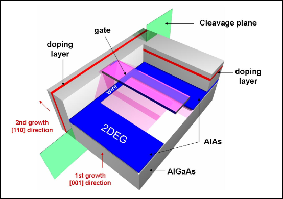
Figure 4.1: Aluminum arsenide quantum wire fabricated using the cleaved edge overgrowth technique. The notation 2DEG refers to the two dimensional electron gas which couples to the quantum wire from either side. Picture courtesy of Dr. M. Rother, Ph.D Thesis (2000), Technische Universitaet Muenchen, Germany.

A theoretical attempt has been made in this direction by Starykh et.al. Starykh where they examined and demonstrated the possibility of gapped phases in a QWR focusing on the nested bandstructure arrangement (see Fig. 4.2) which arises due to the quantum confinement. According to their theoretical proposal when the electronic density in such a system is tuned so that the lowest two successive energy levels are occupied, there are gapped phases possible, for e.g., an interband CDW, with anti-correlated charge density waves in each band, and a “Cooper phase” at zero pairing momenta with strong singlet superconducting fluctuations. However due to the possibility of density reorganization (see Fig 4.2) a mechanism in which it becomes energetically favorable for the two lowest subbands to match their densities, the interband CDW is the most likely state. The Cooper phase may exist just as the second band becomes occupied, when the difference in Fermi momenta is the largest Starykh .

In this regard one of the questions which could be posed is the following: Is there a possibility of a robust superconducting phase with a spin gap in a multiple Fermi point QWR? To answer the question we consider the theoretical treatment of an AlAs QWR which has been recently fabricated by Moser et.al. JM ; Moser using the cleaved edge overgrowth technique Yacoby (see Fig. 4.1). Our calculations indicate that in the clean limit (i.e. no disorder) this QWR has the possibility to realize a spin gap with a stable SS phase with finite pairing momentum. The finite pairing of the Cooper pairs is an indication of a Fulde-Ferrell-Larkin-Ovchinnikov (FFLO) state which is known to lead to inhomogeneous superconductivitycasalbuoni:263 .

AlAs is a heavy mass semiconductor with three degenerate valleys in the first Brillouin zone and anisotropic mass shayegan-2006 . The arrangement of the bands in momentum-space makes it an ideal candidate for a system where multiple Fermi points are present even at the lowest densities. There are two degenerate nonoverlapping bands separated in momentum-space by half an umklapp vector ($k_{U}$), as illustrated in Fig. 4.3. For low densities with only the lowest bands of transverse quantization occupied, the density-reorganizing interband CDW instability discussed above is forbidden. In addition, since the two (degenerate) band minima are connected by half an umklapp vector, there is a class of umklapp excitations unique to this bandstructure which exist at all densities (see Fig. 4.5(e)) and which have the possibility to favor novel electronic phases.

\psfrag{E}{E}\psfrag{k}{k}\includegraphics[width=144.54pt]{fig4_ppt.EPS}

Figure 4.2: Bandstructure of a quantum wire where there is only one band of lowest energy. When the first two bands are filled, interactions between the four Fermi points lead to gaps. The possibility of density reorganization is shown, in which it becomes energeticaly favorable for the first two subbands to match their Fermi momenta. This costs the kinetic energy of moving the densities away from the noninteracting values, but gains the CDW gap energy Starykh . The notations $E$ and $k$ refer to energy and momentum respectively.

In this chapter, we use abelian bosonization and the weak coupling renormalization group scheme to theoretically characterize this QWR. We find that for repulsive interactions, the wire can be tuned so that the ground state has a spin gap which favors either a divergent CDW correlation function or a divergent singlet superconducting correlation function with finite pairing momenta for the Cooper pairs. Even though the original problem contains a repulsive electron-electron interaction, there is a possibility of generating an effective attraction between the electrons in the course of renormalization of the electron-electron interaction. Such a repulsion induced superconductivity is a novel realization in itself and the fact that a mesoscopic system such as the AlAs QWR discussed in this dissertation can allow for its physical realization is a great source of excitement. The final phase has one gapless (total) charge mode with no gapless spin modes. In the literature this is also referred to as the C1S0 phase Varma ; Balents ; spingap ; Starykh .

The outline of this chapter is as follows. In section II we describe the AlAs bandstructure. In section III we state the model Hamiltonian used to describe the AlAs QWR and classify the low energy long wavelength fermionic interaction processes which are important. In section IV we bosonize the Hamiltonian in a symmetric and an anti-symmetric basis of the bosonic fields constructed from the two bands $A$ and $B$ (see Fig. 4.3(b)). In section V we derive the renormalization group equations and discuss the electronic phase diagram. In section VI we state the conclusions.

II Quantum wire bandstructure

In bulk AlAs, conduction-band minima (or valleys) occur at the six equivalent X-points of the Brillouin zone. The constant energy surface consists of six half ellipsoids (three full ellipsoids in the first Brillouin zone), with their major axes along one of the $\langle 100\rangle$ directions. These valleys are highly anisotropic with an anisotropic effective mass of 1.1$m_{e}$ in the longitudinal direction and 0.19$m_{e}$ in the transverse direction, where $m_{e}$ is the bare mass of the electron. Since a large effective mass leads to a reduced kinetic energy, many-body effects related to the Coulomb potential are expected to be enhanced in AlAs compared to the light-mass, 0.067$m_{e}$, GaAs system.

In the AlAs QWR fabricated by the cleaved edge overgrowth process Yacoby ; JM , the initial growth direction is along [001] with the AlAs layer flanked by GaAs and AlGaAs on either side. This creates the two dimensional electron gas. To prepare the QWR the heterostructure is then cleaved in the perpendicular direction specified by [110] (the cleavage plane). The 1D channel thus formed at the edge of the cleaved plane together with the tantulum gate deposited on top of the two dimensional electron gas then helps to define the length of the QWR.

The bandstructure of the QWR can be estimated, approximately, by taking slices through the bandstructure of the corresponding two or three dimensional material. For special systems such as CNTs, which have cylindrical boundary conditions one can just take slices with various transverse momenta which is a good quantum number in these systems. However, most other physical systems do not have such elegant boundary conditions, and in general there will be boundary reflections that mix states of different transverse momenta. The effect of this is that the dispersion of the lowest lying band, rather than corresponding to a slice along a particular constant transverse momentum, corresponds instead to a slice that tracks the minimum of the two or three dimensional dispersion relation.

\psfrag{x}{X-valley}\psfrag{y}{Y-valley}\psfrag{g}{$\Gamma$}\psfrag{kx}{$k_{x}$}\psfrag{ky}{$k_{y}$}\includegraphics[width=180.67499pt]{fabdetails.EPS}

(a) Two valleys, four Fermi points

\psfrag{k}{k}\psfrag{E}{E}\psfrag{umk}{$\frac{k_{U}}{2}$}\psfrag{A}{A}\psfrag{B}{B}\includegraphics[width=252.94499pt]{fig2_paper.EPS}

(b) Quantum wire bandstructure wire

Figure 4.3: (a)The aluminum arsenide quantum wire bandstructure considered here has the four Fermi points indicated in the diagram. The two ellipses refer to the degenerate X and Y valleys Shkolnikov situated at the X-point (indicated by the open circle) of the Brillouin zone. Note the energy minimum for aluminum arsenide is not at the $\Gamma$-point. The distance between the two open circles is half an umklapp vector. (b)In our calculation the quantum wire bandstructure is modelled with the two degenerate bands labeled A and B referring to the degenerate X and Y valleys in an aluminum arsenide bandstructure. Even at the lowest densities, there are two degenerate subbands. In addition, the band minima are separated by half an umklapp vector, $k_{U}/2$, giving rise to new “umklapp” interactions which are present at all fillings. The Fermi points, represented by black dots on the figure, are at $k^{A\pm}_{F}=-\frac{k_{U}}{4}\pm k^{o}_{F}$ and $k^{B\pm}_{F}=\frac{k_{U}}{4}\pm k^{o}_{F}$ where $k_{U}$ is the umklapp vector, and $k_{F}^{o}$ is the magnitude of the Fermi wavevector measured from the bottom of each band. The notations $E$ and $k$ refer to energy and momentum respectively.

For the cleaved edge AlAs QWR when one performs this analysis yloh we obtain the bandstructure arrangement as shown in Fig. 4.3(b). In the lowest lying band the transverse momentum has no role to play. The bandstructure consists of two degenerate bands $A$ and $B$, as shown in Fig. 4.3(b), referring to the degenerate X and Y valleys in the AlAs bandstructure (see Fig. 4.3(a)). Even at the lowest densities, there are two degenerate subbands. In addition, the band minima are separated by half an umklapp vector, $k_{U}/2$, giving rise to umklapp interactions which are present at all fillings and is not related to the commensurability of the electron gas with the underlying lattice. The four Fermi points, represented by black dots in Fig. 4.3(a) and Fig. 4.3(b), are at $k^{A\pm}_{F}=-\frac{k_{U}}{4}\pm k^{o}_{F}$ and $k^{B\pm}_{F}=\frac{k_{U}}{4}\pm k^{o}_{F}$ where $k_{U}$ is the umklapp vector, and $k_{F}^{o}$ is the magnitude of the Fermi wavevector measured from the bottom of each band.

We also note that the band structure of AlAs electrons is similar to Si, except that in Si there are six ellipsoids centered around six equivalent points along the $\Delta$-lines of the Brillouin zone, while in AlAs we have three (six half) ellipsoids at the $X$-points. Typically these valleys are denoted by the directions of their major axes: $X,Y,$ and $Z$ for the [100], [010], and [001] valleys, respectively. For our purposes a crucial difference between AlAs and Si is the manner in which the valleys are occupied in a quantum well from which eventually the QWRs are fabricated. When the electrons are confined along the [001] direction in a (001) Si-MOSFET or a Si/Si-Ge heterostructure, the two $Z$ valleys, with their major axes pointing out of plane, are occupied because the larger mass of electrons along the confinement direction lowers their energy. In AlAs quantum wells grown on a (001) GaAs substrate, however, the $Z$ valley is occupied only if the well thickness is less than approximately 5 $nm$ Gunawan . For larger well thicknesses, a biaxial compression of the AlAs layer, induced by the lattice mismatch between AlAs and GaAs, causes the $X$ and $Y$ valleys with their major axes lying in the plane to be occupied shayegan-2006 . For the AlAs QWR fabricated by Moser et.al. JM using the cleaved edge overgrowth technique (see Fig. 4.3), the well thickness is 15 $nm$. As a result the $X$ and $Y$ valleys are lower in energy and provide the two degenerate conduction bands which can be occupied by electrons. For Si such a possibility is precluded as stated above.

There are also crucial differences between the AlAs QWR and the CNT bandstructure. In the CNTs the two bands, around the Dirac points, between which the electron-electron scattering processes take place are not separated by half an umklapp vector as in the AlAs QWR BalentsFisher . Furthermore, the umklapp interactions which are generated in the CNT systems are present only at half-fillings and not just at any electronic density. At half-filling, a metallic CNT maps to the Hubbard model also at half-filling. While the Hubbard model has umklapps at half-filling, these do not correspond to umklapps in the original CNT. Rather, they are merely extra interactions which are only allowed by symmetry at the Dirac points, i.e. at half-filling. Also, a metallic tube is unlike our QWR, in that the pseudospin which is equivalent to the sublattice quantum number prevents an electron from backscattering from one branch to another around the same Brillouin zone points. A doped semiconducting tube could perhaps do this. We in fact do include backscattering within the same subband which is strictly forbidden in a metallic CNT.

Furthermore, empirical evidence Gunawan ; Shkolnikov suggests that in an AlAs quantum well the spin degeneracy is not lifted in the absence of magnetic field leading us to conclude that spin-orbit coupling effects can be safely ignored in the theoretical formulation of the present problem.

III The Fermionic Hamiltonian

In a QWR electrons are quantum mechanically confined to move along one direction with their motion in the remaining transverse directions confined via a potential $V_{conf}(\vec{r_{\perp}})$ where $\vec{r}_{\perp}=(y,z)$ denotes the transverse coordinates of quantization. Electron-electron interactions within the wire are described by $U(\vec{r}$) which is purely repulsive. The Hamiltonian is a sum of two independent terms in the transverse and longitudinal directions with the result that the wavefunction (and therefore the correlation functions) can be decomposed as a product of $\phi(\vec{r}_{\perp})$ and $\psi_{s}(x)$ where $\phi(\vec{r}_{\perp})$ is the orthogonal wavefunction of transverse quantization of the two degenerate bands ($X$ and $Y$ valleys) and $\psi_{s}(x)$ the longitudinal part. In order to describe the physics along the longitudinal direction we now promote the wavefunction, $\psi_{s}(x)$, to the level of a field operator (for a field theoretic description) responsible for creating and annihilating the electrons taking part in the various scattering processes. With this in mind the second quantized Hamiltonian suitable for our purposes of study is

$$H=\sum_{s}\int d^{3}r\Psi^{{\dagger}}_{s}(\vec{r})\left(-\frac{1}{2m}\vec{\nabla}^{2}_{r}-\mu+V_{conf}(\vec{r}_{\perp})\right)\Psi_{s}(\vec{r})$$

$$+\frac{1}{2}\sum_{s,s^{{}^{\prime}}}\int d^{3}rd^{3}r^{{}^{\prime}}U(\vec{r}-\vec{r^{{}^{\prime}}})\Psi^{{\dagger}}_{s}(\vec{r})\Psi^{{\dagger}}_{s^{{}^{\prime}}}(\vec{r}^{{}^{\prime}})\Psi_{s^{{}^{\prime}}}(\vec{r}^{{}^{\prime}})\Psi_{s}(\vec{r})$$ (4.1)

where $\Psi_{s}(\vec{r})=\phi(\vec{r}_{\perp})\psi_{s}(x)$ is now the field operator for an electron species of spin $s=\{\uparrow,\downarrow$}, and $\mu$ is the chemical potential in the leads. Because the low energy, long wavelength excitations occur around the vicinity of the Fermi points (see Fig. 4.3(b)) a further decomposition is possible with $\Psi_{s}(\vec{r})=\phi(\vec{r}_{\perp})(\psi_{As}(x)+\psi_{Bs}(x))$. The coordinate $x$ is in the long direction of the wire. The longitudinal part of the field can be naturally expanded in terms of the right- and left- moving excitations, $R_{ns}(x)$ and ${L}_{ns}(x)$, respectively, residing around the Fermi points of the two bands (indicated by the black dots in Fig. 4.3(b)) with $\psi_{As}(x)=R_{As}(x)e^{ik^{A+}_{F}x}+L_{As}(x)e^{ik^{A-}_{F}x}$ and $\psi_{Bs}(x)=R_{Bs}(x)e^{ik^{B+}_{F}x}+L_{Bs}(x)e^{ik^{B-}_{F}x}$. The band index is $n=A,B$ and the Fermi momenta are defined by $k^{A\pm}_{F}=-\frac{k_{U}}{4}\pm k^{o}_{F}$ and $k^{B\pm}_{F}=\frac{k_{U}}{4}\pm k^{o}_{F}$ where $k_{U}$ is the umklapp vector, and $k_{F}^{o}$ is the magnitude of the Fermi wavevector measured from the bottom of each band, as shown in Fig. 4.3(b).

The interaction part of the Hamiltonian reduces to a sum of two types of fermionic processes. The first type describes the interaction of electrons within the same band, $n=A,B$, and contains the forward $(U^{F}_{intra})$ and the backward scattering $(U^{B}_{intra})$ processes. These are referred to as the intraband interaction processes. The second type describes electron-electron scattering processes involving both bands, classified as interband interactions. The relevant interband interaction terms in the fermionic language include forward (U^F), backward $(U^{B}_{d},U^{B}_{x}$ and $U^{B}_{inter})$, and inter-valley umklapp $(U_{um}$) scattering. The Fermionic interaction terms of the problem are expressed below via the right- and left- moving excitations, $R_{ns}(x)$ and $L_{ns}(x)$. In the interaction terms stated below the band index is $n=A,B$, the spin index is $s=\{\uparrow,\downarrow\}$, $k_{U}$ is the umklapp vector and $k_{F}^{o}$ is the magnitude of the Fermi wavevector measured from the bottom of each band as shown in Fig. 4.3(b). The notation $\xi_{n}=\delta_{nA}-\delta_{nB}$. The matrix element $M$, which is the interaction kernel, is given by the expression

$$M(x-x^{{}^{\prime}})=\int U(\vec{r}-\vec{r}^{{}^{\prime}})\phi^{2}(\vec{r}_{\perp})\phi^{2}(\vec{r}^{{}^{\prime}}_{\perp})d\vec{r}_{\perp}d\vec{r}^{{}^{\prime}}_{\perp}.$$ (4.2)

The Fermionic interaction terms are as follows

Intraband interaction (see Fig. 4.4)

The intraband forward and backward scattering terms are shown in Fig. 4.4 and their expressions stated in Eqs. 4.3 and  4.4. The intraband forward scattering interaction term, $U^{F}_{intra}$, is

$$U^{F}_{intra}=\frac{1}{2}\sum_{n=A,B}\int dxdx^{{}^{\prime}}M(x-x^{{}^{\prime}})\sum_{s,s^{{}^{\prime}}}\bigg{[}R^{{\dagger}}_{ns}(x)R_{ns}(x)+L^{{\dagger}}_{ns}(x)L_{ns}(x)\bigg{]}$$

$$\times\bigg{[}R^{{\dagger}}_{ns^{{}^{\prime}}}(x^{{}^{\prime}})R_{ns^{{}^{\prime}}}(x^{{}^{\prime}})+L^{{\dagger}}_{ns^{{}^{\prime}}}(x^{{}^{\prime}})L_{ns^{{}^{\prime}}}(x^{{}^{\prime}})\bigg{]}$$ (4.3)

\psfrag{E}{E}\psfrag{k}{k}\includegraphics[width=252.94499pt]{intraforward.EPS}

(a) Intraband forward scattering ($U^{F}_{intra}$)

\psfrag{E}{E}\psfrag{k}{k}\includegraphics[width=252.94499pt]{intrabackscattering.EPS}

(b) Intraband backscattering ($U^{B}_{intra}$)

Figure 4.4: Representative low energy long wavelength intraband electron-electron scattering processes. In each figure $E$ and $k$ refer to energy and momentum respectively. The open and filled dots represent electrons which are taking part in the scattering processes with the arrows depicting the direction of scattering. The Fermi points are at $k^{A\pm}_{F}=-\frac{k_{U}}{4}\pm k^{o}_{F}$ and $k^{B\pm}_{F}=\frac{k_{U}}{4}\pm k^{o}_{F}$ (as described in Fig. 4.3(b)) where $k_{U}$ is the umklapp vector, and $k_{F}^{o}$ is the magnitude of the Fermi wavevector measured from the bottom of each band.

and the intraband backscattering term, $U^{B}_{intra}$ is

$$U^{B}_{intra}=\frac{1}{2}\sum_{n=A,B}\int dxdx^{{}^{\prime}}M(x-x^{{}^{\prime}})\sum_{s,s^{{}^{\prime}}}\bigg{[}R^{{\dagger}}_{ns}(x)L^{{\dagger}}_{ns^{{}^{\prime}}}(x^{{}^{\prime}})R_{ns^{{}^{\prime}}}(x^{{}^{\prime}})L_{ns}(x)e^{-2ik^{o}_{F}(x-x^{{}^{\prime}})}$$

$$+L^{{\dagger}}_{ns}(x)R^{{\dagger}}_{ns^{{}^{\prime}}}(x^{{}^{\prime}})L_{ns^{{}^{\prime}}}(x^{{}^{\prime}})R_{ns}(x)e^{2ik^{o}_{F}(x-x^{{}^{\prime}})}\bigg{]}$$ (4.4)

The interband scattering terms are shown in Fig. 4.5 and their expressions stated in Eqs. 4.5 –  LABEL:eqn:umklapcooper.

Interband interaction

(see Fig. 4.5)

The forward scattering term, $U^{F}$, is

$$U^{F}=\frac{1}{2}\sum_{n\neq m}\int dxdx^{{}^{\prime}}M(x-x^{{}^{\prime}})\sum_{s,s^{{}^{\prime}}}\bigg{[}R^{{\dagger}}_{ns}(x)R_{ns}(x)+L^{{\dagger}}_{ns}(x)L_{ns}(x)\bigg{]}$$

$$\times\bigg{[}R^{{\dagger}}_{ms^{{}^{\prime}}}(x^{{}^{\prime}})R_{ms^{{}^{\prime}}}(x^{{}^{\prime}})+L^{{\dagger}}_{ms^{{}^{\prime}}}(x^{{}^{\prime}})L_{ms^{{}^{\prime}}}(x^{{}^{\prime}})\bigg{]}$$ (4.5)

The direct backscattering term, $U^{B}_{d}$, is

$$U^{B}_{d}=\frac{1}{2}\sum_{n\neq m}\int dxdx^{{}^{\prime}}M(x-x^{{}^{\prime}})\sum_{s,s^{{}^{\prime}}}\bigg{[}R^{{\dagger}}_{ns}(x)L_{ns}(x)L^{{\dagger}}_{ms^{{}^{\prime}}}(x^{{}^{\prime}})R_{ms^{{}^{\prime}}}(x^{{}^{\prime}})e^{-2ik^{o}_{F}(x-x^{{}^{\prime}})}$$

$$+L^{{\dagger}}_{ns}(x)R_{ns}(x)R^{{\dagger}}_{ms^{{}^{\prime}}}(x^{{}^{\prime}})L_{ms^{{}^{\prime}}}(x^{{}^{\prime}})e^{2ik^{o}_{F}(x-x^{{}^{\prime}})}\bigg{]}$$

(4.6)

The exchange backscattering term, $U^{B}_{x}$, is

$$U^{B}_{x}=-\frac{1}{2}\sum_{n\neq m}\int dxdx^{{}^{\prime}}M(x-x^{{}^{\prime}})e^{i\frac{k_{U}}{2}(x-x^{{}^{\prime}})\xi_{n}}\sum_{s,s^{{}^{\prime}}}\bigg{[}R^{{\dagger}}_{ns}(x)L_{ns^{{}^{\prime}}}(x^{{}^{\prime}})L^{{\dagger}}_{ms^{{}^{\prime}}}(x^{{}^{\prime}})R_{ms}(x)$$

$$+L^{{\dagger}}_{ns}(x)R_{ns^{{}^{\prime}}}(x^{{}^{\prime}})R^{{\dagger}}_{ms^{{}^{\prime}}}(x^{{}^{\prime}})L_{ms}(x)\bigg{]}$$

(4.7)

The interband backscattering term, $U^{B}_{inter}$, is

$$U^{B}_{inter}=-\frac{1}{2}\sum_{n\neq m}\int dxdx^{{}^{\prime}}M(x-x^{{}^{\prime}})e^{i\frac{k_{U}}{2}(x-x^{{}^{\prime}})\xi_{n}}\sum_{s,s^{{}^{\prime}}}\bigg{[}R^{{\dagger}}_{ns}(x)R_{ns^{{}^{\prime}}}(x^{{}^{\prime}})R^{{\dagger}}_{ms^{{}^{\prime}}}(x^{{}^{\prime}})R_{ms}(x)$$

$$+L^{{\dagger}}_{ns}(x)L_{ns^{{}^{\prime}}}(x^{{}^{\prime}})L^{{\dagger}}_{ms^{{}^{\prime}}}(x^{{}^{\prime}})L_{ms}(x)+R^{{\dagger}}_{ns}(x)R_{ns^{{}^{\prime}}}(x^{{}^{\prime}})L^{{\dagger}}_{ms^{{}^{\prime}}}(x^{{}^{\prime}})L_{ms}(x)e^{-i2k^{o}_{F}(x-x^{{}^{\prime}})}$$

$$+L^{{\dagger}}_{ns}(x)L_{ns^{{}^{\prime}}}(x^{{}^{\prime}})R^{{\dagger}}_{ms^{{}^{\prime}}}(x^{{}^{\prime}})R_{ms}(x)e^{i2k^{o}_{F}(x-x^{{}^{\prime}})}\bigg{]}$$

(4.8)

and finally the inter-valley umklapp scattering term, $U_{um}$, is

$$U_{um}=\frac{1}{2}\sum_{n\neq m}\int dxdx^{{}^{\prime}}M(x-x^{{}^{\prime}})e^{i\frac{k_{U}}{2}(x-x^{{}^{\prime}})\xi_{n}}\sum_{s,s^{{}^{\prime}}}\bigg{[}R^{{\dagger}}_{ns}(x)L^{{\dagger}}_{ns^{{}^{\prime}}}(x^{{}^{\prime}})e^{-ik^{o}_{F}(x-x^{{}^{\prime}})}$$

$$+ L^{{\dagger}}_{ns}(x)R^{{\dagger}}_{ns^{{}^{\prime}}}(x^{{}^{\prime}})e^{ik^{o}_{F}(x-x^{{}^{\prime}})}\bigg{]}\bigg{[}R_{ms^{{}^{\prime}}}(x^{{}^{\prime}})L_{ms}(x)e^{-ik^{o}_{F}(x-x^{{}^{\prime}})}+L_{ms^{{}^{\prime}}}(x^{{}^{\prime}})R_{ms}(x)e^{ik^{o}_{F}(x-x^{{}^{\prime}})}\bigg{]}$$

\psfrag{E}{E}\psfrag{k}{k}\includegraphics[width=252.94499pt]{fig8_ppt.EPS}

(a) Forward scattering ($U^{F}$)

\psfrag{E}{E}\psfrag{k}{k}\includegraphics[width=252.94499pt]{fig6_ppt.EPS}

(b) Direct backscattering ($U^{B}_{d}$)

\psfrag{E}{E}\psfrag{k}{k}\includegraphics[width=252.94499pt]{fig9_ppt.EPS}

(c) Exchange backscattering ($U^{B}_{x}$)

\psfrag{k}{k}\psfrag{E}{E}\includegraphics[width=252.94499pt]{fig10_ppt.EPS}

(d) Interband backscattering ($U^{B}_{inter}$)

\psfrag{E}{E}\psfrag{k}{k}\includegraphics[width=252.94499pt]{fig7_ppt.EPS}

(e) Inter-valley umklapp scattering ($U_{um}$)

Figure 4.5: Representative low energy long wavelength interband electron-electron scattering processes. In each figure $E$ and $k$ refer to energy and momentum respectively. The open and filled dots represent electrons which are taking part in the scattering processes with the arrows depicting the direction of scattering. The Fermi points are at $k^{A\pm}_{F}=-\frac{k_{U}}{4}\pm k^{o}_{F}$ and $k^{B\pm}_{F}=\frac{k_{U}}{4}\pm k^{o}_{F}$ (as described in Fig. 4.3(b)) where $k_{U}$ is the umklapp vector, and $k_{F}^{o}$ is the magnitude of the Fermi wavevector measured from the bottom of each band. The inter-valley umklapp scattering (Fig. 4.5(e)) shown above is unique to this aluminum arsenide quantum wire bandstructure arrangement.

The interband forward scattering term is shown in Fig. 4.5(a). The backscattering term has three types - direct, exchange and interband. We define direct backscattering, U${}^{B}_{d}$, as an event where backscattering processes occur in each band separately (see Fig. 4.5(b)). Exchange backscattering, U${}^{B}_{x}$, has the same initial and final states as direct backscattering, but the electrons switch bands (see Fig. 4.5(c)). Interband backscattering, $U^{B}_{inter}$, is backscattering between two electrons in different bands (see Fig. 4.5(d)). The inter-valley umklapp scattering is unique to this bandstructure (see Fig. 4.5(e)). It is a scattering process where two electrons starting, for e.g., in band A with total momentum -$k_{U}$/2 scatter into band B, with total momentum $k_{U}$/2. The momentum difference between the initial and final states is an umklapp vector which can be exchanged with the lattice. This is an umklapp process which is present at all densities and is not related to the commensurability of the electron gas with the underlying lattice. It is unique to the AlAs QWR bandstructure and as we shall see later will play an important role in classifying the phase diagram.

IV Bosonizing the Hamiltonian

The low energy properties of the interacting 1D electron gas can be conveniently described within the framework of the bosonization technique Miranda ; Giamarchi ; Gogolin ; Devreese . Within this approach one can associate with the right- and left- moving, ${R}_{ns}(x)$ and ${L}_{ns}(x)$, respectively, fermionic field operators a combination of bosonic fields $\phi_{n\nu}=(\phi_{n\uparrow}\pm\phi_{n\downarrow})/\sqrt{2}$ and $\theta_{n\nu}=(\theta_{n\uparrow}\pm\theta_{n\downarrow})/\sqrt{2}$, where $\nu=\rho,\sigma$ (the charge and spin modes) correspond to the $\pm$ combination, $s=\{\uparrow,\downarrow$} is the spin index and $n=A,B$ is the band index. The bosonic fields satisfy the commutation relation [$\phi_{n\nu}(x),\partial_{x^{{}^{\prime}}}\theta_{n^{{}^{\prime}}\nu^{{}^{\prime}}}(x^{{}^{\prime}})$]=i$\pi\delta(x-x^{{}^{\prime}})\delta_{\nu,\nu^{{}^{\prime}}}\delta_{n,n^{{}^{\prime}}}$ with $\hbar$ set equal to one. We then have

$${R}_{ns}(x)=\frac{\eta_{Rns}}{\sqrt{2\pi\alpha}}e^{i\sqrt{\pi\over 2}[\theta_{n\rho}(x)-\phi_{n\rho}(x)+s(\theta_{n\sigma}(x)-\phi_{n\sigma}(x))]}$$ (4.10)

and,

$${L}_{ns}(x)=\frac{\eta_{Lns}}{\sqrt{2\pi\alpha}}e^{i\sqrt{\pi\over 2}[\theta_{n\rho}(x)+\phi_{n\rho}(x)+s(\theta_{n\sigma}(x)+\phi_{n\sigma}(x))]}$$ (4.11)

where $\alpha$ is the short distance cutoff, $\eta_{Rns}$ and $F_{Lns}$ are the Klein factors for the right- and left- moving fields of band $n$ with species of spin $s$. They are required to preserve the anti-commutation relations of the fermionic fields. The convenient field variables for the Hamiltonian in our problem will be a linear combination of the boson fields constructed out of the two bands. We define the transformation to a symmetric and an anti-symmetric basis as $\phi^{\pm}_{\nu}=\frac{1}{\sqrt{2}}(\phi_{A\nu}\pm\phi_{B\nu})$ and $\theta^{\pm}_{\nu}=\frac{1}{\sqrt{2}}(\theta_{A\nu}\pm\theta_{B\nu})$. Upon bosonization and subsequent transformation the parts of the Hamiltonian corresponding to free motion produce the harmonic terms in the symmetric and the anti-symmetric bosonic fields $(\phi^{\pm}_{\nu}$ and $\theta^{\pm}_{\nu})$ only. The intraband interactions and the interband interactions, however, generate both cosine interaction terms and harmonic terms. Furthermore while bosonizing we also used the fact that the exponential $e^{ik_{U}x}=1$. This is true because the electrons in the QWR move in an underlying lattice and their spatial coordinate $x=ma_{x}$, where $a_{x}$ is the lattice spacing in the long direction of the wire and $m$ is an integer. When multiplied with the umklapp vector, $k_{U}=2\pi/a_{x}$, and exponentiated the result is $\exp[-2m\pi]=1$.

The Hamiltonian, $H$, can be written in the following canonical form

$$H=\frac{1}{2}\sum_{\mu=\pm}\sum_{\nu=\rho,\sigma}\int dR\bigg{[}v^{\mu}_{\nu}K^{\mu}_{\nu}(\partial_{R}\theta^{\mu}_{\nu})^{2}+\frac{v^{\mu}_{\nu}}{K^{\mu}_{\nu}}(\partial_{R}\phi^{\mu}_{\nu})^{2}\bigg{]}+H_{int}$$ (4.12)

where the bosonic interaction terms, $H_{int}$, are

$$H_{int}=\frac{t_{1}}{2\pi^{2}\alpha^{2}}\int dR\cos[\sqrt{4\pi}\phi^{+}_{\sigma}]\cos[\sqrt{4\pi}\phi^{-}_{\sigma}]$$

$$+\frac{t_{2}}{2\pi^{2}\alpha^{2}}\int dR\cos[\sqrt{4\pi}\phi^{-}_{\rho}]\cos[\sqrt{4\pi}\phi^{+}_{\sigma}]$$

$$+\frac{t_{3}}{2\pi^{2}\alpha^{2}}\int dR\cos[\sqrt{4\pi}\phi^{-}_{\rho}]\cos[\sqrt{4\pi}\phi^{-}_{\sigma}]$$

$$+\frac{t_{4}}{2\pi^{2}\alpha^{2}}\int dR\cos[\sqrt{4\pi}\phi^{-}_{\rho}]\cos[\sqrt{4\pi}\theta^{-}_{\sigma}]$$

$$+\frac{t_{5}}{2\pi^{2}\alpha^{2}}\int dR\cos[\sqrt{4\pi}\theta^{-}_{\sigma}]\cos[\sqrt{4\pi}\phi^{-}_{\sigma}]$$

$$+\frac{t_{6}}{2\pi^{2}\alpha^{2}}\int dR\cos[\sqrt{4\pi}\theta^{-}_{\sigma}]\cos[\sqrt{4\pi}\phi^{+}_{\sigma}]$$

$$+\frac{t_{7}}{2\pi^{2}\alpha^{2}}\int dR\sin[\sqrt{4\pi}\theta^{-}_{\sigma}]\sin[\sqrt{4\pi}\phi^{+}_{\sigma}]$$

$$+\frac{t_{8}}{2\pi^{2}\alpha^{2}}\int dR\cos[\sqrt{4\pi}\theta^{-}_{\rho}]\cos[\sqrt{4\pi}\theta^{-}_{\sigma}]$$

$$+\frac{t_{9}}{2\pi^{2}\alpha^{2}}\int dR\cos[\sqrt{4\pi}\theta^{-}_{\rho}]\cos[\sqrt{4\pi}\phi^{+}_{\sigma}]$$

$$+\frac{t_{10}}{2\pi^{2}\alpha^{2}}\int dR\cos[\sqrt{4\pi}\theta^{-}_{\rho}]\cos[\sqrt{4\pi}\phi^{-}_{\sigma}]$$

$$+\frac{t_{11}}{2\pi^{2}\alpha^{2}}\int dR\cos[\sqrt{4\pi}\theta^{-}_{\rho}]\cos[\sqrt{4\pi}\phi^{-}_{\rho}]$$ (4.13)

with the coupling constants defined in terms of the Coulomb matrix element $M(a)$

$$t_{1}=t_{2}=2\int daM(a)\cos[2k^{o}_{F}a]$$

$$t_{3}=2\int daM(a)\bigg{(}\cos[2k^{o}_{F}a]-\cos\bigg{[}\frac{k_{U}a}{2}\bigg{]}\bigg{)}$$

$$t_{4}=t_{5}=-t_{10}=-t_{11}=-2\int M(a)\cos\bigg{[}\frac{k_{U}a}{2}\bigg{]}$$

$$t_{6}=-t_{9}=-2\int daM(a)\cos[2k^{o}_{F}a]\cos\bigg{[}\frac{k_{U}a}{2}\bigg{]}$$

$$t_{7}=-2\int daM(a)\sin[2k^{o}_{F}a]\sin\bigg{[}\frac{k_{U}a}{2}\bigg{]}$$

$$t_{8}=2\int daM(a)\bigg{(}1-\cos[2k^{o}_{F}a]\bigg{)}\cos\bigg{[}\frac{k_{U}a}{2}\bigg{]}$$ (4.14)

In the Hamiltonian, $R=(x+x^{{}^{\prime}})/2$ is the center-of-mass coordinate of two electrons and $a=x-x^{{}^{\prime}}$ their relative coordinate in the long direction of the QWR. In the quadratic part the bare symmetric and anti-symmetric Luttinger parameters, $K^{\pm}_{\nu}$, quoted in appendix Appendix A: Luttinger parameters for the quantum wire, can be expressed in terms of the original Luttinger parameters $K_{\nu}$. Furthermore the Luttinger parameters which have been derived here starting from the Fermionic Hamiltonian, Eq. III, are the bare effective parametersGiamarchi . The symmetric and anti-symmetric velocities $v^{\pm}_{\nu}$, refer appendix Appendix A: Luttinger parameters for the quantum wire, can also be expressed in terms of the original velocities $v_{\nu}$.

The coupling constants of the problem are denoted by $t_{i}$, where $i=1,\dots,11$. They are related to the fourier components of the interaction kernel, $M(a)$, with the wavevectors of the problem - $k_{U}$ and $k_{F}^{o}$. It is instructive to observe that the umklapp vector is independent of the electron density in the QWR whereas $k_{F}^{o}$ is not. This allows for the interesting possibility to tune $k_{F}^{o}$ experimentally and control the initial conditions in the renormalization group equations itself and possibly get oneself into various electronic phases of matter as allowed in an interacting 1D electron gas problem. Also, the initial conditions depend on the QWR parameters - the width ($w$), the length $(L)$, and the distance of the QWR from the back-gate $(d)$.

The first bosonized interaction term with the coupling $t_{1}$ arises from intraband backscattering type processes (refer Fig. 4.4(b)) with a coupling strength which depends on the $2k_{F}^{o}$ cosine fourier component of the interaction kernel $M(a)$. The second is a result of the direct backscattering type interaction as shown in Fig. 4.5(b) and has a coupling strength equal to that of an intraband backscattering process. This is evident from the diagram of the scattering processes shown in Figs. 4.4(b) and  4.5(b). The third interaction term has contributions from both the direct and exchange backscattering processes, whereas the fourth term is exclusively generated from exchange backscattering. The exchange backscattering process has a strength which depends on the $k_{U}/2$ cosine fourier component of the interaction kernel $M(a)$. The third interaction term is a combination of both and has the $2k_{F}^{o}$ and the $k_{U}/2$ cosine fourier components. These first four interaction terms have in their bosonized expressions the charge density wave phase $\phi_{\rho}^{-}$ for the relative charge channel in the antisymmetric basis together with the spin fields $\phi_{\sigma}^{+},\phi_{\sigma}^{-}$, and $\theta_{\sigma}^{-}$. The next three terms $t_{5},t_{6}$, and $t_{7}$ are generated from the interband backscattering process shown in Fig. 4.5(d). They involve only the spin fields $\phi_{\sigma}^{+},\phi_{\sigma}^{-}$, and $\theta_{\sigma}^{-}$. For $t_{6}$ and $t_{7}$ the coupling depends on both the $2k_{F}^{o}$ and $k_{U}/2$ cosine fourier component of the interaction kernel. The strength of $t_{5}$ is proportional to $\frac{k_{U}}{2}$.

Bosonization of the inter-valley umklapp scattering fermionic processes produce six bosonized interaction terms in total. Out of those, two are of the form

$$\sim\cos[\sqrt{4\pi}\theta^{-}_{\rho}]\cos[\sqrt{4\pi}\phi^{-}_{\rho}]\cos[\sqrt{4\pi}\theta^{-}_{\sigma}]\cos[\sqrt{4\pi}\phi^{-}_{\sigma}]$$

$$\sim\sin[\sqrt{4\pi}\theta^{-}_{\rho}]\sin[\sqrt{4\pi}\phi^{-}_{\rho}]\sin[\sqrt{4\pi}\theta^{-}_{\sigma}]\sin[\sqrt{4\pi}\phi^{-}_{\sigma}]$$ (4.15)

From a purely physical standpoint these terms involve self destructing competing dual fields. Furthermore the couplings associated with these interactions can never grow since the perturbations involved have a scaling dimension which is greater than two and makes them irrelevant in the renormalization group sense. We therefore ignore their contribution in computing the renormalization group equations. We retain only the remaining four interaction terms labeled as $t_{8},t_{9},t_{10}$ and $t_{11}$. All these terms involve the superconducting phase $\theta_{\rho}^{-}$ for the relative charge channel in the anti-symmetric basis togther with the spin fields of the problem. Their coupling strength depends on the $2k_{F}^{o}$ and $k_{U}/2$ cosine fourier component. Finally we note that the Hamiltonian remains quadratic in the total charge fields $\phi_{\rho}^{+}$ and $\theta_{\rho}^{+}$.

In summary, starting from the interacting 1D Hamiltonian (see Eq. III) we have classified the important low energy long wavelength fermionic interaction processes and then bosonized them (see Eqs. 4.12 and  IV). In the next section V we use a weak coupling renormalization group treatment, described earlier in chapter 3, to determine which of the coupling constants associated with the bosonized interaction terms diverge.

V Analyzing the renormalization group equations

To analyze the low energy, long wavelength behavior of the interacting system, we employ the renormalization group approach. In this approach the shortwavelength modes are systematically eliminated leading to a set of coupled differential equations for the coupling constants. For the present problem, one can derive the appropriate renormalization group equations for the entire set of interactions, $t_{i}$, where $i=1,\dots,11$, in perturbation theory about the noninteracting fixed point, the quadratic Hamiltonian Eq. 4.12 using the momentum shell renormalization group procedure described in chapter 3. The renormalization group equations for these coupling constants (up to second order, $\mathcal{O}(2)$) of the problem are quoted in appendix Appendix B: Renormalization group equations.

We study the renormalization group equations for the regimes - $K^{-}_{\rho}<1$ (repulsive) and $K^{-}_{\rho}>1$ (attractive) of the bosonic theory in the relative charge channel. The $K^{-}_{\rho}<1$ case is repulsive since it promotes the CDW phase, $\phi^{-}_{\rho}$. The $K^{-}_{\rho}>1$ case is attractive because it promotes the SS phase, $\theta^{-}_{\rho}$. The equations are integrated numerically for some suitable initial conditions until one or more couplings grow to be of order one, $\mathcal{O}(1)$. The order one $\mathcal{O}(1)$ couplings are considered to be large and thus pin (gap) the appropriate bosonic modes. We then replace the gapped fields with their expectation value both in the Hamiltonian and in the bosonized version of the correlation functions. The correlation functions which do not vanish then help to determine the divergent susceptibilities and the possible thermodynamic phase for that regime.

The initial condition under which we begin the renormalization group flow is determined by evaluating the coupling constants, Eq. IV, for the QWR parameters width, length and the distance from the back-gate. The phenomenological form for the interaction kernel is $M(a)=\frac{e^{2}}{4\pi\epsilon_{o}}\frac{e^{-(a/d)}}{\sqrt{w^{2}+a^{2}}}$, which has the nature of a screened Coulomb potential where $e$ is the electronic charge and $\epsilon_{o}$ the permittivity of free space. The screening involves two length scales. The distance of the QWR to the back-gate, $d$, and the width, $w$, of the wire. The width $w$ provides the short-distance cutoff whereas the distance to the back-gate $d$ is the long-distance cutoff. Using these parameters and the expression for the coupling constants, Eq. IV, we can make an estimate for the initial conditions.

For the quantum wire of Moser et.al.JM ; Moser we have a transverse size of $w\sim 15nm$ separated from the metallic gate by a distance $d\sim 300nm$. The wire length is $L\sim 1\mu m$. We then have $w/d\sim$ 0.05 and the ratio $L/d$ = 10/3. The parameters used to estimate $k^{o}_{F}$ for the aluminum arsenide bandstructure are: density of the electrons in the quantum wire $\sim 10^{8}m^{-1}$ and the effective mass of the electron $m^{*}=0.33m_{e}$ along the long direction where $m_{e}$ is the bare mass of the electron JM . Furthermore, experimental evidence Gunawan ; Shkolnikov suggests that spin rotational invariance is not broken in the AlAs quantum wells in the absence of a magnetic field. The problem is then $SU(2)$ invariant and we can set $K^{\pm}_{\sigma}=1$ to begin the renormalization group flow.

The analysis, with the above initial conditions, for the repulsive regime in the relative charge channel, $K_{\rho}^{-}<1$, shows that the coupling constants $t_{2}$ and $t_{3}$ diverge, in fact $(t_{2},t_{3})\rightarrow(\infty,\infty)$. The fields which get gapped are the antisymmetric charge field $\phi^{-}_{\rho}$ and the spin fields $\phi^{\pm}_{\sigma}$. Their possible acquired expectation values are $(\langle\phi^{-}_{\rho}\rangle,\langle\phi^{+}_{\sigma}\rangle,\langle\phi^{-}_{\sigma}\rangle)$=$(\pm\sqrt{\pi}/2,0,0)$ or $(0,\pm\sqrt{\pi}/2,\pm\sqrt{\pi}/2)$. The final phase in either case is a dominant divergent intraband (odd combination) 2$k^{o}_{F}$-CDW. The corresponding $CDW$ correlation function, $\hat{O}^{intra,odd}_{CDW,2k^{o}_{F}}$ (refer appendix Appendix C: Correlation functions for the quantum wire), decays with the power law $\chi_{CDW}\sim(1/r)^{K^{+}_{\rho}/2}$ where $K_{\rho}^{+}$ is the total charge Luttinger parameter.

Although the original screened Coulomb interaction is repulsive, in the course of renormalization it can be led to an effective attractive regime, $K_{\rho}^{-}>1$. For this case the renormalization group flows indicate that the divergent coupling constants are $t_{9}$ and $t_{10}$ where both $(t_{9},t_{10})\rightarrow(\infty,\infty)$. From the interactions terms we can then deduce that the dual antisymmetric charge field $\theta_{\rho}^{-}$ gets gapped together with the spin fields $\phi^{\pm}_{\sigma}$. They acquire the expectation values of $(\langle\theta^{-}_{\rho}\rangle,\langle\phi^{+}_{\sigma}\rangle,\langle\phi^{-}_{\sigma}\rangle)$=$(\pm\sqrt{\pi}/2,0,0)$ or $(0,\pm\sqrt{\pi}/2,\pm\sqrt{\pi}/2)$. These gapped fields lead to a state with a divergent intraband SS correlation function $\Delta^{intra,singlet}$ (appendix Appendix C: Correlation functions for the quantum wire) with the power law $\chi_{SS}\sim(1/r)^{1/2K^{+}_{\rho}}$.

We also find through our analysis that although for the finite sized wire with $L/d\sim 3.33$, the initial conditions for the renormalization group flows differ from the true 1D limit of $L/d\rightarrow\infty$, due to the screening of the back gate this is not a severe effect, and the system remains in the same basin of attraction as the infinite wire. The renormalization group results can now be summarized in the phase diagram shown in Fig. 4.6

\psfrag{intra}{Intraband}\psfrag{inter}{Intraband}\psfrag{Krho1}{$K^{-}_{\rho}<1$}\psfrag{eqn}{$2k_{F}^{o}-CDW$}\psfrag{Krho2}{$K^{-}_{\rho}>1$}\psfrag{sing}{SS}\psfrag{kpneq}{$(k_{p}\neq 0)$}\psfrag{1}{1}\psfrag{krho}{$K_{\rho}^{-}$}\includegraphics[width=216.81pt]{QWRphasediagram.EPS}

Figure 4.6: Phase diagram: Divergent correlation functions for the quantum wire in the presence of inter-valley umklapp scattering for the two regimes K${}^{-}_{\rho}<$ 1 (repulsive) and K${}^{-}_{\rho}>$ 1 (attractive). The notation CDW stands for charge density wave and SS for singlet superconducitvity. In the diagram $k_{p}$ denotes the pairing momenta of the center-of-mass of the Cooper pairs. The finite pairing momentum is an indication of a Fulde-Ferrell-Larkin-Ovchinnikov (FFLO) state which is encouraged in this wire due to the presence of the umklapp interactions. Such a state is also known to lead to inhomogeneous superconductivity.

For the AlAs QWR bandstructure, due to the presence of four Fermi points we have in general eight fields, $\phi^{\pm}_{\nu}$ and their duals $\theta^{\pm}_{\nu}$ where $\nu=\rho,\sigma$ refer to the charge and spin modes. For a gapless system, Luttinger liquid, we would have a C2S2 phase where the notation refers to the number of gapless charge $(C)$ and spin $(S)$ modes. But in the present problem due to the presence of interactions certain modes as predicted by the renormalization analysis get gapped. Furthermore, due to the absence of any bosonized interaction terms in the total charge mode we expect the total charge field to remain gapless. As a result we have the C1S0 phase Varma ; Balents where the notation refers to one gapless total charge mode $(\phi^{+}_{\rho})$ with all other charge and spin modes gapped.

One of the novel aspects of this superconductivity is that it originated from a purely repulsive screened Coulomb interaction. In the process of renormalization, in the relative charge channel for $K^{-}_{\rho}>1$, an attractive interaction was generated. This resulted in a pairing of up and down spins within a band and subsequent scattering of it from one band to another via the umklapp Cooper scattering process. Energetically the process can be understood as a competition between Coulomb repulsion of pairing and the kinetic energy of the pair where the latter wins. Such a kinetic energy driven mechanism for superconductivity has been proposed earlier in the context of high temperature superconductorsspingap .

Another unique aspect of this superconductivity is that the pairing momenta of the Cooper pairs is nonzero. It is half the umklapp vector. Being at a finite wavevector one could think of this as a density modulated superconducting state where the superfluid density varies from one lattice site to another with the wavevector $\frac{k_{U}}{2}$. Such an inhomogeneous superconducting state is known to arise in the FFLO state casalbuoni:263 .

VI Conclusion

QWRs provide an opportunity for technological innovation. In this context a phase diagram helps to understand what electronic phase the QWR may predominantly find itself in since it has an important effect on the transport properties. In this paper we have investigated the possibility of a spin gapped AlAs QWR. Using 1D field theoretic methods and perturbative renormalization group we are able to conclude that the novel AlAs QWR, fabricated by Moser et al. Moser ; JM under investigation will have the possibility of a spin gapped state with divergent 2$k^{o}_{F}$-CDW or SS fluctuations. While the CDW wave phase is robust deep in the repulsive region, there is a part of the phase diagram which promotes a non-trivial SS with finite-momentum Cooper pairing leading to an inhomogeneous superconducting state. The finite pairing momentum is an indication of a FFLO state.

Chapter 5 LUTTINGER LIQUID KINK

I Introduction

One of the most dramatic consequences of confining electrons to one spatial dimension is the prediction of spin-charge separation. That is, due to many-body interactions the electron is no longer a stable quasiparticle, but decays into separate spin and charge modes tomonaga1950 ; luttinger1960 ; mattis-lieb1965 . A direct experimental observation of spin-charge separation has proven difficult although evidence for Luttinger liquid behavior has been reported in many 1D systems, via, e.g., a suppression of the density of states near the Fermi level in ropes of carbon nanotubesbockrath-smalley1997 or power law behavior in the conductance vs. temperature in edge states of the fractional quantum Hall effectmilliken-webb1996 ; chang1996 and carbon nanotubesbockrath-smalley1999 . Until now, very limited direct evidence for spin-charge separation has been reported. Tunneling measurements later provided evidence for explicit spin-charge separation in 1D systems, via real-space imaging of Friedel oscillations using scanning tunneling microscopy on single-walled carbon nanotubeslee-eggert2004 and momentum- and energy-resolved tunneling between two coupled QWRsauslaender-halperin2005 , both of which observed multiple velocities indicative of spin-charge separation. More direct evidence of spin-charge separation would be to measure separate spin and charge dispersions in a single-particle spectral function.zx-2006 Despite much effort in this area, this has only been achieved recently in an unambiguous way in the Mott-Hubbard insulator SrCuO₂.zx-2006 Other claims of the detection of separately dispersing spin and charge peaks with ARPESclaessen1995 ; segovia1999 have been overturnedbluebronze-not ; Si-Au-not , or lack independent verification of the spin and charge energy scales.TTF-TCNQ

Part of the difficulty in directly measuring spin and charge dispersions through measurements proportional to the single particle spectral function is that within Luttinger liquid theory, the spinon branch is muted compared to the holon branch. Finite temperature and experimental resolution only compound the problem, making direct detection of the spinon branch in, e.g., ARPES difficult. In this chapter, we show how spin-charge separation can nevertheless be detected via the systematic temperature dependence of a kink in the effective electronic dispersion, even in cases where the spin peak is not directly resolvable.

\psfrag{B}{Binding Energy}\psfrag{m}{Momentum}\psfrag{vs}{$v_{\sigma}$}\psfrag{vc}{$v_{\rho}$}\includegraphics[width=289.07999pt]{ThermalBroaden.EPS}

Figure 5.1: Schematic diagram of peak broadening due to interactions and finite temperature in the Luttinger liquid spectral function. The dashed lines denote the zero temperature dispersion tracking the charge part with velocity $v_{\rho}$ and the spin part with velocity $v_{\sigma}$. At $T\neq 0$, the peaks become thermally broadened as indicated by the shaded regions. In this case the effective dispersion now tracks the solid red line, so that the low energy part tracks the sum of the two broad spin and charge peaks, resulting in a low energy velocity $v_{l}$ which is between the spin and charge velocities. Note the high energy effective dispersion is parallel to the charge part but displaced, an effect due to finite temperature and interactions. This results in the high energy part extrapolating back to a value $k_{ex}\neq k_{F}$.

II Theory

Although the electron is not an elementary excitation of the Luttinger liquid because it is unstable to spin-charge separation, an effective electronic dispersion may still be defined by the existence of (generally broad) peaks in the spectral function. At zero temperature in 1D, there are two sharp peaks in the electronic spectral function, one dispersing at the velocity $v_{\sigma}$ of the collective spin modes (spinons) and the other at the velocity $v_{\rho}$ of the collective charge modes (holons)meden1992 ; voit1993 . However, at finite temperature, the spin and charge peaks are broadened, as shown schematically in Fig. 5.1. At low binding energy, this causes the two to merge into one broad peak with an effective dispersion which lies between the spin velocity $v_{\sigma}$ and the charge velocity $v_{\rho}$. Although the two peaks separate at higher binding energies, interactions and temperature strongly suppress the spin peak for repulsive interactions. As a result, the dominant (and most easily measurable) peak will disperse with the charge velocity at high energy. This gives rise to a kink in the effective electronic dispersion. Since the Luttinger liquid is quantum critical, the kink energy scales linearly with temperature, $E_{\rm kink}\propto a(r,\gamma_{\rho})T$, where $a$ is a function of the velocity ratio $r=v_{\sigma}/v_{\rho}$ and the interaction strength $\gamma_{\rho}=\frac{1}{8}(K_{\rho}+K_{\rho}^{-1}-2)$ where $K_{\rho}$ is the charge Luttinger parameter. For $\gamma_{\rho}=0.15-0.30$ and $r=0.2-0.4$, the range of $a$ is $a=3.3-3.9$. The kink is stronger for lower values of $r$, but diminishes again for strong enough interaction strength. Moreover, the high energy linear effective dispersion extrapolates to the Fermi energy at a wavevector $k_{ex}\neq k_{F}$ which is shifted from the Fermi wavevector by an amount which scales linearly with temperature. Recently explicit analytic expressions for correlation functions in the Tomonaga-Luttinger liquid at finite temperature were obtained under various conditionsOrgad . We consider here the single hole spectral function, $A^{<}(k,\omega)$, since it is directly proportional to the intensity observed in ARPES experiments. In the spin-rotationally invariant case, the finite-temperature single hole spectral functionOrgad may be written in terms of the scaled variables $\tilde{k}=\frac{v_{s}k}{\pi T}$ and $\tilde{\omega}=\frac{\omega}{\pi T}$ with the Boltzmann constant $k_{B}=1$,

$$A^{<}(\tilde{k},\tilde{\omega})\propto\int^{\infty}_{-\infty}dq~{}h_{\frac{1}{2}}(\tilde{k}-2rq)\times$$

$$h_{\gamma_{c}+\frac{1}{2}}\bigg{[}{\tilde{\omega}-\tilde{k}\over 2}+(1+r)q\bigg{]}h_{\gamma_{c}}\bigg{[}{\tilde{\omega}-\tilde{k}\over 2}-(1-r)q\bigg{]}$$

where $r=v_{\sigma}/v_{\rho}$ is the ratio between the spin velocity and the charge velocity and $h_{\gamma}$ is related to the beta function

$$h_{\gamma}(k)=\Re e\bigg{[}(2i)^{\gamma}B\bigg{(}\frac{\gamma-ik}{2},1-\gamma\bigg{)}\bigg{]}$$ (5.2)

The charge interaction strength $\gamma_{\rho}$ is related to the charge Luttinger parameter $K_{\rho}$ by $\gamma_{\rho}=\frac{1}{8}(K_{\rho}+K_{\rho}^{-1}-2)$, i.e. $\gamma_{\rho}=0$ in the noninteracting case, and $\gamma_{\rho}$ increases with increasing interaction strength. Because of spin rotation invariance, we use $K_{\sigma}=1$ and $\gamma_{\sigma}=0$.

III Results and Discussion

In order to define a single-hole effective dispersion, we use momentum distribution curves (MDC’s), i.e. the single hole spectral function $A^{<}(k,\omega_{o})$ considered as a function of $k$ at a given value of the frequency $\omega_{o}$. The effective dispersion is identified by the position $k_{o}=k_{o}(\omega_{o})$ of the maximum of $A_{\rm max}^{<}(k,\omega_{o})$ with respect to $k$. This gives an implicit equation for the effective single hole dispersion $\omega_{o}(k_{o})$. This method gives a more reliable definition of the effective dispersion than using energy distribution curves (EDC’s), i.e. the spectral function considered as a function of frequency at a given momentum $k_{o}$, $A^{<}(k_{o},\omega)$. Whereas EDC’s can become quite broad with increasing interaction strength, MDC’s are always sharp due to kinematic constraints,frac so that there is less experimental uncertainty in identifying the location of a peak in the MDC.

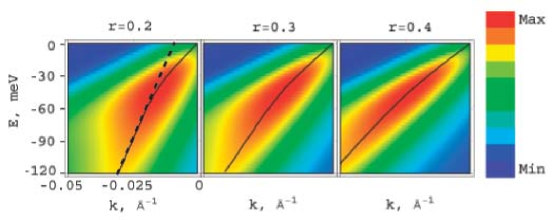
(a)  $A^{<}(k,\omega)$ at $\gamma_{\rho}=0.15$

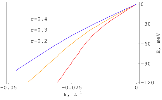
(b)  Effective dispersion at $\gamma_{\rho}=0.15$

Figure 5.2: Intensity of the spectral function $A^{<}(k,\omega)$ and effective dispersions at an interaction strength $\gamma_{\rho}=0.15$. (a) The intensity of $A^{<}(k,\omega)$ is shown for three different ratios of the spin to charge velocity, $r=0.2,~{}0.3,$ and $0.4$. The black lines are the effective electronic dispersions derived from MDC peaks, as described in the text. The dashed line in the first panel shows that the high energy part of the effective dispersion does not extrapolate back to the Fermi wavevector, $k_{F}$. (b) Comparison of the dispersions at different values of the velocity ratio, $r=0.2,~{}0.3,$ and $0.4$. In all cases the spin velocity $v_{\sigma}=1$eV-$\AA$ and the temperature $k_{B}T=14meV$.

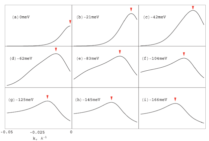
Figure 5.3: MDC’s for $\gamma_{\rho}=0.15$. The spin velocity $v_{\sigma}=1$eV-$\AA$ and the temperature $k_{B}T=14meV$. The ratio of spin to charge velocity is $r=0.2$.

Fig. 5.2(a) shows representative intensity plots of the spectral function, $A^{<}(k,\omega)$. In the figure, we have used an interaction strength $\gamma_{\rho}=0.15$, temperature $k_{B}T=14$meV, and velocity ratios $r=0.2$, $0.3$, and $0.4$. Fig 5.3 shows the corresponding MDC’s for $r=0.2$, plotted as a function of momentum $k$ at a few representative energies. The red triangles show the position of the maximum of the MDC curves. The resulting effective dispersion is denoted by the solid black lines in Fig. 5.2(a). As is evident from the figure, the effective dispersion is linear as expected at low energy and also at high energy, but with different velocities. This gives rise to a “kink” in the effective dispersion, i.e. a change in the effective velocity. While at zero temperature, there are two well-defined peaks in the MDC’s, one dispersing with the charge velocity and the other with the spin velocity, when the temperature is finite, the width of these MDC peaks is thermally broadened. (See Fig. 5.1.) At low energies and finite temperatures, the sum of the two broad peaks is itself one broad peak, as can be seen in panels (a)-(c) in Fig. 5.3, and the maximum in the MDC will track a velocity $v_{l}$ which is between the spin and charge velocities, $v_{\sigma}<v_{l}<v_{\rho}$. At high enough energies, the temperature broadened singularities due to the spin and charge part become sufficiently separated, and the spin peak is sufficiently muted, that the MDC peak tracks the charge velocity. The separation of the muted spin peak from the stronger charge peak can be seen in panels (d) and (e) of Fig. 5.3. In panels (f)-(i), the charge and spin peaks have moved sufficiently apart that the peak in the MDC will track the charge part. Aside from the presence of a kink in the effective dispersion, the position of the high energy linear effective dispersion is another signature of Luttinger liquid behavior. In Fig. 5.2(a), the dotted line is an extrapolation of the high energy linear part of the effective dispersion back to the Fermi energy. As can be seen from the figure, the dotted line extrapolates to $E=E_{F}$ at a wavevector $k_{ex}=k_{F}+\alpha(r,\gamma_{\rho})T$ which is shifted from the Fermi wavevector by an amount which scales linearly with temperature.

Fig. 5.2(b) shows the effective dispersion for each of the three values of $r$, overlaid for comparison. As one might expect, as $r\rightarrow 1$, the kink vanishes, since then the charge and spin pieces disperse with the same velocity. As $r$ is decreased, so that now $v_{\rho}>v_{\sigma}$, a kink appears, and strengthens as $r$ is further decreased. One can see the general features that the low energy part disperses with a velocity $v_{l}$ which is between the spin and charge velocities, $v_{\sigma}<v_{l}<v_{\rho}$, and that the high energy part disperses with the charge velocity. However, this high energy effective dispersion extrapolates back to the Fermi energy at a wavevector $k_{ex}\neq k_{F}$. At higher interaction strengths, EDC’s broaden significantly, so that $k_{ex}$ is smaller and the kink diminishes in strength. However, $E_{\rm kink}$ moves to deeper binding energy as the interaction strength is increased. Additional calculations exploring the dependence of the kink on various interaction strengths are shown in appendix Appendix D: Variation of Luttinger liquid kink with interaction strength.

In Fig. 5.4 we show how the effective dispersion changes with temperature. Because the Luttinger liquid is quantum critical, the spectral function has a scaling form, and the only energy scale in the effective dispersion is the temperature itself. As a result, the kink energy depends linearly on the temperature, $E_{\rm kink}\propto T$. As can be seen in the figure, varying only the temperature merely moves the kink to deeper binding energy, leaving the low energy velocity $v_{l}$ (and therefore the strength of the kink) unchanged. in addition, as temperature is increased, the high energy part extrapolates back to the Fermi energy at a higher value of $k_{ex}$.

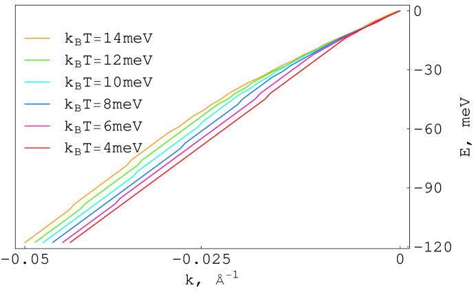
Figure 5.4: Temperature variation of the effective dispersion. The temperature varies from $k_{B}T=4$meV to $k_{B}T=14$meV, starting from the lower curve and moving to the upper curve. The interaction strength $\gamma_{\rho}=0.15$, the spin velocity $v_{\sigma}=1$eV-$\AA$, and the ratio of spin to charge velocity $r=0.3$.

Up until now, we have studied the Luttinger kink in a phenomenological manner, allowing $\gamma_{\rho}$ and $r$ to vary independently of each other. It is also useful to consider the systematics of the kink strength and energy within the context of a microscopic model. As an example, we show in Fig. 5.5 results for a Luttinger liquid derived from an incommensurate repulsive 1D Hubbard model. We take the density to be away from half filling, $n=0.3$. For a given value of $U/t$, renormalized values of $\gamma_{c}^{*}$ and $r^{*}$ are taken from Ref. schulz1995 , where Bethe-ansatz was used to find the renormalized values of $K_{\rho}^{*}$, $v_{\rho}^{*}$, and $v_{\sigma}^{*}$. In Fig. 5.5, we show the intensity plots of the spectral function along with the effective dispersion, for the values $U/t=16,8,$ and $4$ of the repulsive Hubbard model. This corresponds to renormalized values of $\gamma_{\rho}^{*}=0.05,0.04,0.02$, and $r^{*}=0.1,0.2,0.4$, respectively. Upon increasing the Hubbard interaction strength $U$, the strength of the kink is enhanced due to the change in the renormalized velocity ratio $r^{*}$. Notice that in this case, the kink is more pronounced, and there is a sharper distinction between the low energy and high energy linear parts.

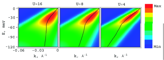
(a)  $A^{<}(k,\omega)$ as $U$ varies

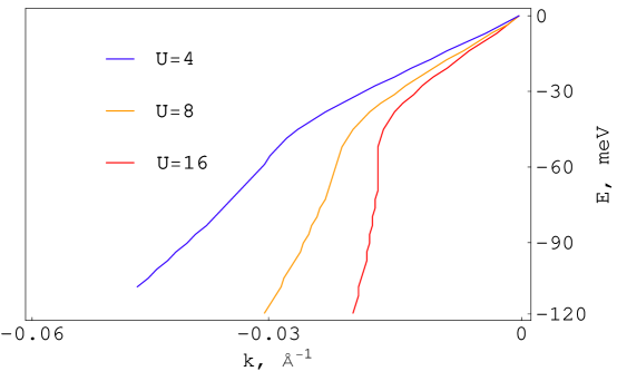
(b)  Effective dispersion as $U$ varies

Figure 5.5: Intensity of the spectral function $A^{<}(k,\omega)$ and effective dispersions for $U=16,8,$ and $4$ in units of the hopping integral $t$. The density $n=0.3$. (a) The intensity of $A^{<}(k,\omega)$. The black lines are the effective electronic dispersions derived from MDC peaks, as described in the text. (b) Comparison of the dispersions at different values of $U/t$. In all cases the spin velocity $v_{\sigma}=1$eV-$\AA$ and the temperature $k_{B}T=14meV$.

It is worth noting that behavior reminiscent of this physics was recently reported in ARPES experiments on the quasi-one-dimensional Mott-Hubbard insulator SrCuO₂.zx-2006 Being an insulating material, SrCuO₂ is gapped, whereas the Luttinger spectral functions presented here are not. Nevertheless, the effective dispersion (measured by EDC’s) shows a single peak at energies close to the gap, which then separates into two peaks at higher binding energy.

IV Conclusion

In conclusion, we have shown the existence of a temperature-dependent kink in the effective electronic dispersion of a spin-rotationally invariant Luttinger liquid, due to spin-charge separation. At low energies, the effective dispersion is linear, with a velocity between the spin and charge velocities, $v_{\sigma}<v_{l}<v_{\rho}$. At high energies, the MDC peak disperses with the charge velocity. Because the Luttinger liquid is quantum critical, the kink between the high energy and low energy behavior has an energy set by temperature, $E_{\rm kink}\propto T$. In addition, the high energy effective dispersion extrapolates back to the Fermi energy at a wavevector $k_{ex}\neq k_{F}$ which is shifted from the Fermi wavevector by an amount which is proportional to temperature. As interactions are increased, the kink diminishes in strength, and moves to higher binding energy. In cases where finite temperature and interactions along with experimental uncertainties obscure the detection of two separate peaks in the effective dispersion, the kink analysis presented here can be used as a signature of spin-charge separation in Luttinger liquids.

APPENDICES oddAPPENDICESy0pt

Appendix A: Luttinger parameters for the quantum wire

The symmetric and the anti-symmetric velocity ($v^{\pm}_{\rho}$,$v^{\pm}_{\sigma}$) and the Luttinger parameters, ($K^{\pm}_{\rho}$,$K^{\pm}_{\sigma}$) are expressed in terms of the original velocity and the Luttinger parameters as

$$v^{+}_{\rho}K^{+}_{\rho}=v_{\rho}K_{\rho}+\frac{M(2k^{o}_{F})}{2\pi}-\frac{b^{-}}{2\pi}$$ (A.1)

$$\frac{v^{+}_{\rho}}{K^{+}_{\rho}}=\frac{v_{\rho}}{K_{\rho}}+\frac{8M(0)-M(2k^{o}_{F})}{2\pi}-\frac{b^{+}}{2\pi}$$ (A.2)

$$v^{-}_{\rho}K^{-}_{\rho}=v_{\rho}K_{\rho}+\frac{M(2k^{o}_{F})}{2\pi}+\frac{b^{-}}{2\pi}$$ (A.3)

$$\frac{v^{-}_{\rho}}{K^{-}_{\rho}}=\frac{v_{\rho}}{K_{\rho}}-\frac{M(2k^{o}_{F})}{2\pi}+\frac{b^{+}}{2\pi}$$ (A.4)

$$v^{+}_{\sigma}K^{+}_{\sigma}=v_{\sigma}K_{\sigma}+\frac{M(2k^{o}_{F})}{2\pi}-\frac{b^{-}}{2\pi}$$ (A.5)

$$\frac{v^{+}_{\sigma}}{K^{+}_{\sigma}}=\frac{v_{\sigma}}{K_{\sigma}}-\frac{M(2k^{o}_{F})}{2\pi}-\frac{b^{+}}{2\pi}$$ (A.6)

$$v^{-}_{\sigma}K^{-}_{\sigma}=v_{\sigma}K_{\sigma}+\frac{M(2k^{o}_{F})}{2\pi}+\frac{b^{-}}{2\pi}$$ (A.7)

$$\frac{v^{-}_{\sigma}}{K^{-}_{\sigma}}=\frac{v_{\sigma}}{K_{\sigma}}-\frac{M(2k^{o}_{F})}{2\pi}+\frac{b^{+}}{2\pi}$$ (A.8)

where the $b^{\pm}$ are defined as

$$b^{\pm}=\pm\frac{e^{2}}{4\pi\epsilon_{o}}\int da\frac{e^{-(a/d)}\cos\bigg{[}\frac{k_{U}a}{2}\bigg{]}(M(2k^{o}_{F})\pm M(0))}{\sqrt{w^{2}+a^{2}}}$$ (A.9)

and $M(0)=\int daM(a)$ and $M(2k^{o}_{F})=\int daM(a)\cos[2k^{o}_{F}a]$. The interaction kernel is $M(a)=\frac{e^{2}}{4\pi\epsilon_{o}}\frac{e^{-(a/d)}}{\sqrt{w^{2}+a^{2}}}$ (see Eq. 4.2) where $a$ is the distance along the long direction of the wire, $e$ is the electronic charge, and $\epsilon_{o}$ the permittivity of free space. The phenomenological charge and spin Luttinger parameters are $K_{\rho}$ and $K_{\sigma}$ respectively, and the charge and the spin velocities are $v_{\rho}$ and $v_{\sigma}$. The velocities are taken to be identical for the two bands since they are degenerate. The explicit expressions for the bare Luttinger parameters and the bare velocities are given by

$$K_{\nu}=\sqrt{\frac{2\pi v_{F}+2g_{4,\nu}+g_{\nu}}{2\pi v_{F}+2g_{4,\nu}-g_{\nu}}}$$ (A.10)

and

$$v_{\nu}=\sqrt{\bigg{(}v_{F}+\frac{g_{4,\nu}}{\pi}\bigg{)}^{2}-\bigg{(}\frac{g_{\nu}}{2\pi}\bigg{)}^{2}}$$ (A.11)

where $g_{\rho}=g_{1}-2g_{2},g_{\sigma}=g_{1},g_{4,\rho}=g_{4}$ and $g_{4,\sigma}=0$. In terms of the forward and backscattering amplitudes the above g-ology coefficients are given by $g_{1}=M(2k^{o}_{F}),g_{2}=M(0)-M(2k^{o}_{F})$ and $g_{4}=M(0)$. The wavevectors $k_{U}$ and $k_{F}^{o}$, respectively, are the umklapp wavevector and the magnitude of the Fermi wavevector measured from the bottom of each band (see Fig. 4.3).

Appendix B: Renormalization group equations

The renormalization group equation for the coupling constants (see Eq. IV) of the problem are

$$\frac{dt_{1}}{dL}=\bigg{(}2-K^{+}_{\sigma}-K^{-}_{\sigma}\bigg{)}t_{1}-\frac{t_{2}t_{3}}{2\pi}-\frac{t_{5}t_{6}}{2\pi}-\frac{t_{9}t_{10}}{2\pi}$$ (B.1)

$$\frac{dt_{2}}{dL}=\bigg{(}2-K^{-}_{\rho}-K^{+}_{\sigma}\bigg{)}t_{2}-\frac{t_{1}t_{3}}{2\pi}-\frac{t_{4}t_{6}}{2\pi}-\frac{t_{9}t_{11}}{2\pi}$$ (B.2)

$$\frac{dt_{3}}{dL}=\bigg{(}2-K^{-}_{\rho}-K^{-}_{\sigma}\bigg{)}t_{3}-\frac{t_{1}t_{2}}{2\pi}-\frac{t_{4}t_{5}}{2\pi}-\frac{t_{10}t_{11}}{2\pi}$$ (B.3)

$$\frac{dt_{4}}{dL}=\bigg{(}2-\frac{1}{K^{-}_{\sigma}}-K^{-}_{\rho}\bigg{)}t_{4}-\frac{t_{2}t_{6}}{2\pi}-\frac{t_{3}t_{5}}{2\pi}-\frac{t_{8}t_{11}}{2\pi}$$ (B.4)

$$\frac{dt_{5}}{dL}=\bigg{(}2-\frac{1}{K^{-}_{\sigma}}-K^{-}_{\sigma}\bigg{)}t_{5}-\frac{t_{1}t_{6}}{2\pi}-\frac{t_{3}t_{4}}{2\pi}-\frac{t_{8}t_{10}}{2\pi}$$ (B.5)

$$\frac{dt_{6}}{dL}=\bigg{(}2-\frac{1}{K^{-}_{\sigma}}-K^{+}_{\sigma}\bigg{)}t_{6}-\frac{t_{1}t_{5}}{2\pi}-\frac{t_{2}t_{4}}{2\pi}-\frac{t_{8}t_{9}}{2\pi}$$ (B.6)

$$\frac{dt_{7}}{dL}=\bigg{(}2-\frac{1}{K^{-}_{\sigma}}-K^{+}_{\sigma}\bigg{)}t_{7}$$ (B.7)

$$\frac{dt_{8}}{dL}=\bigg{(}2-\frac{1}{K^{-}_{\rho}}-\frac{1}{K^{-}_{\sigma}}\bigg{)}t_{8}-\frac{t_{4}t_{11}}{2\pi}-\frac{t_{5}t_{10}}{2\pi}-\frac{t_{6}t_{9}}{2\pi}$$ (B.8)

$$\frac{dt_{9}}{dL}=\bigg{(}2-\frac{1}{K^{-}_{\rho}}-{K^{+}_{\sigma}}\bigg{)}t_{9}-\frac{t_{1}t_{10}}{2\pi}-\frac{t_{2}t_{11}}{2\pi}-\frac{t_{6}t_{8}}{2\pi}$$ (B.9)

$$\frac{dt_{10}}{dL}=\bigg{(}2-K^{-}_{\sigma}-\frac{1}{K^{-}_{\rho}}\bigg{)}t_{10}-\frac{t_{1}t_{9}}{2\pi}-\frac{t_{3}t_{11}}{2\pi}-\frac{t_{5}t_{8}}{2\pi}$$ (B.10)

$$\frac{dt_{11}}{dL}=\bigg{(}2-K^{-}_{\rho}-\frac{1}{K^{-}_{\rho}}\bigg{)}t_{11}-\frac{t_{2}t_{9}}{2\pi}-\frac{t_{3}t_{10}}{2\pi}-\frac{t_{4}t_{8}}{2\pi}$$ (B.11)

$$\frac{d\ln K^{-}_{\rho}}{dL}=\frac{1}{8\pi^{2}}\bigg{[}-K^{-}_{\rho}\bigg{(}t^{2}_{2}+t^{2}_{3}+t^{2}_{4}\bigg{)}+\frac{1}{K^{-}_{\rho}}\bigg{(}t^{2}_{8}+t^{2}_{9}+t^{2}_{10}+t^{2}_{11}\bigg{)}\bigg{]}$$ (B.12)

$$\frac{d\ln K^{+}_{\sigma}}{dL}=-\frac{K^{+}_{\sigma}}{8\pi^{2}}\bigg{(}t^{2}_{1}+t^{2}_{2}+t^{2}_{6}+t^{2}_{7}+t^{2}_{9}\bigg{)}$$ (B.13)

$$\frac{d\ln K^{-}_{\sigma}}{dL}=\frac{1}{8\pi^{2}}\bigg{[}-K^{-}_{\sigma}\bigg{(}t^{2}_{1}+t^{2}_{3}+t^{2}_{10}+t^{2}_{5}\bigg{)}+\frac{1}{K^{-}_{\sigma}}\bigg{(}t^{2}_{4}+t^{2}_{5}+t^{2}_{6}+t^{2}_{7}+t^{2}_{8}\bigg{)}\bigg{]}$$ (B.14)

where $L=\ln(\Lambda/\alpha)$, with length scale $\Lambda$. The initial conditions of the problem are

$$t_{1}(0)=t_{2}(0)=2\int daM(a)\cos[2k^{o}_{F}a]$$

$$t_{3}(0)=2\int daM(a)\bigg{(}\cos[2k^{o}_{F}a]-\cos\bigg{[}\frac{k_{U}a}{2}\bigg{]}\bigg{)}$$

$$t_{4}(0)=t_{5}(0)=-t_{10}(0)=-t_{11}(0)=-2\int M(a)\cos\bigg{[}\frac{k_{U}a}{2}\bigg{]}$$

$$t_{6}(0)=-t_{9}(0)=-2\int daM(a)\cos[2k^{o}_{F}a]\cos\bigg{[}\frac{k_{U}a}{2}\bigg{]}$$

$$t_{7}(0)=-2\int daM(a)\sin[2k^{o}_{F}a]\sin\bigg{[}\frac{k_{U}a}{2}\bigg{]}$$

$$t_{8}(0)=2\int daM(a)\bigg{(}1-\cos[2k^{o}_{F}a]\bigg{)}\cos\bigg{[}\frac{k_{U}a}{2}\bigg{]}$$ (B.15)

In the above equations the interaction kernel is $M(a)=\frac{e^{2}}{4\pi\epsilon_{o}}\frac{e^{-(a/d)}}{\sqrt{w^{2}+a^{2}}}$ (see Eq. 4.2) where $a$ is the distance along the long direction of the wire. The coupling constants of the interaction terms (see Eq. IV) are denoted by $t_{i}$, where $i=1,\dots,11$. They are related to the fourier components of the interaction kernel, $M(a)$. The wavevectors $k_{U}$ and $k_{F}^{o}$, respectively, are the umklapp wavevector and the magnitude of the Fermi wavevector measured from the bottom of each band (see Fig. 4.3). The symmetric and anti-symmetric velocity ($v^{\pm}_{\rho}$,$v^{\pm}_{\sigma}$) and Luttinger parameters, ($K^{\pm}_{\rho}$,$K^{\pm}_{\sigma}$) are given by the expressions quoted in appendix Appendix A: Luttinger parameters for the quantum wire.

Appendix C: Correlation functions for the quantum wire

The fermionic definition together with the bosonized version of the correlation functions are stated below. The correlation functions have been classified into two categories - intraband and interband. In the expressions the band index is $n=A,B$. The spin index is $s=\{\uparrow,\downarrow$}, and the Fermi momenta are defined by $k^{A\pm}_{F}=-\frac{k_{U}}{4}\pm k^{o}_{F}$ and $k^{B\pm}_{F}=\frac{k_{U}}{4}\pm k^{o}_{F}$ where $k_{U}$ is the umklapp vector, and $k_{F}^{o}$ is the magnitude of the Fermi wavevector measured from the bottom of each band, as shown in Fig. 4.3(b). The correlation functions are expressed in terms of the right- and left- moving excitations, $R_{ns}(x)$ and ${L}_{ns}(x)$, respectively, residing around the Fermi points of the two bands (indicated by the black dots in Fig. 4.3(b)). The fields in the correlation function are the symmetric and the anti-symmetric fields defined as $\phi^{\pm}_{\nu}=\frac{1}{\sqrt{2}}(\phi_{A\nu}\pm\phi_{B\nu})$ and its dual $\theta^{\pm}_{\nu}=\frac{1}{\sqrt{2}}(\theta_{A\nu}\pm\theta_{B\nu})$ where $\nu=\rho,\sigma$ are the charge and spin modes. The Klein factors are denoted by $\eta_{Rns}$ and $\eta_{Lns}$ for the right- and left- moving fermions, respectively, in band $n$ with spin $s$.

C.1 Charge density wave (CDW) correlation functions

Intraband CDW (even combination), $2k_{F}^{o}$ wavevector

$$\hat{O}^{intra,even}_{CDW,2k_{F}^{o}}(x)=[e^{i2k_{F}^{o}x}L^{{\dagger}}_{As}R_{As}+e^{-i2k_{F}^{o}x}R^{{\dagger}}_{As}L_{As}]+(A\rightarrow B)$$ (C.1)

$$=\frac{2}{\pi\alpha}\sin[\sqrt{\pi}(\phi^{+}_{\rho}+\phi^{-}_{\rho})-2k_{F}^{o}x]\cos[\sqrt{\pi}(\phi^{+}_{\sigma}+\phi^{-}_{\sigma})]$$

$$+\frac{2}{\pi\alpha}\sin[\sqrt{\pi}(\phi^{+}_{\rho}-\phi^{-}_{\rho})-2k_{F}^{o}x]\cos[\sqrt{\pi}(\phi^{+}_{\sigma}-\phi^{-}_{\sigma})]$$ (C.2)

Intraband CDW (odd combination), $2k_{F}^{o}$ wavevector

$$\hat{O}^{intra,odd}_{CDW,2k_{F}^{o}}(x)=[e^{i2k_{F}^{o}x}L^{{\dagger}}_{As}R_{As}+e^{-i2k_{F}^{o}x}R^{{\dagger}}_{As}L_{As}]-(A\rightarrow B)$$ (C.3)

$$=\frac{2}{\pi\alpha}\sin[\sqrt{\pi}(\phi^{+}_{\rho}+\phi^{-}_{\rho})-2k_{F}^{o}x]\cos[\sqrt{\pi}(\phi^{+}_{\sigma}+\phi^{-}_{\sigma})]$$

$$-\frac{2}{\pi\alpha}\sin[\sqrt{\pi}(\phi^{+}_{\rho}-\phi^{-}_{\rho})-2k_{F}^{o}x]\cos[\sqrt{\pi}(\phi^{+}_{\sigma}-\phi^{-}_{\sigma})]$$ (C.4)

C.2 Spin density wave (SDW) correlation functions

Intraband SDW (even combination), $2k_{F}^{o}$ wavevector

$$\hat{\vec{O}}^{intra,even}_{SDW,2k_{F}^{o}}(x)=[e^{i2k_{F}^{o}x}L^{{\dagger}}_{A\alpha}\bigg{(}\frac{\vec{\sigma}}{2}\bigg{)}_{\alpha,\beta}R_{A\beta}+e^{-i2k_{F}^{o}x}R^{{\dagger}}_{A\alpha}\bigg{(}\frac{\vec{\sigma}}{2}\bigg{)}^{{\dagger}}_{\alpha,\beta}L_{A\beta}]+(A\rightarrow B)$$ (C.5)

$$[\hat{O}^{intra,even}_{SDW,2k_{F}^{o}}(x)]_{z}=-\frac{1}{\pi\alpha}\cos[\sqrt{\pi}(\phi^{+}_{\rho}+\phi^{-}_{\rho})-2k_{F}^{o}x]\sin[\sqrt{\pi}(\phi^{+}_{\sigma}+\phi^{-}_{\sigma})]$$

$$-\frac{1}{\pi\alpha}\cos[\sqrt{\pi}(\phi^{+}_{\rho}-\phi^{-}_{\rho})-2k_{F}^{o}x]\sin[\sqrt{\pi}(\phi^{+}_{\sigma}-\phi^{-}_{\sigma})]$$ (C.6)

$$[\hat{O}^{intra,even}_{SDW,2k_{F}^{o}}(x)]_{y}=q\frac{1}{\pi\alpha}\cos[\sqrt{\pi}(\phi^{+}_{\rho}+\phi^{-}_{\rho})-2k_{F}^{o}x]\cos[\sqrt{\pi}(\theta^{+}_{\sigma}+\theta^{-}_{\sigma})]$$

$$+\frac{1}{\pi\alpha}\cos[\sqrt{\pi}(\phi^{+}_{\rho}-\phi^{-}_{\rho})-2k_{F}^{o}x]\cos[\sqrt{\pi}(\theta^{+}_{\sigma}-\theta^{-}_{\sigma})]$$ (C.7)

$$[\hat{O}^{intra,even}_{SDW,2k_{F}^{o}}(x)]_{x}=\frac{1}{\pi\alpha}\cos[\sqrt{\pi}(\phi^{+}_{\rho}+\phi^{-}_{\rho})-2k_{F}^{o}x]\sin[\sqrt{\pi}(\theta^{+}_{\sigma}+\theta^{-}_{\sigma})]$$

$$+\frac{1}{\pi\alpha}\cos[\sqrt{\pi}(\phi^{+}_{\rho}-\phi^{-}_{\rho})-2k_{F}^{o}x]\sin[\sqrt{\pi}(\theta^{+}_{\sigma}-\theta^{-}_{\sigma})]$$ (C.8)

Intraband SDW (odd combination), $2k_{F}^{o}$ wavevector

$$\hat{\vec{O}}^{intra,odd}_{SDW,2k_{F}^{o}}(x)=[e^{i2k_{F}^{o}x}L^{{\dagger}}_{A\alpha}\bigg{(}\frac{\vec{\sigma}}{2}\bigg{)}_{\alpha,\beta}R_{A\beta}+e^{-i2k_{F}^{o}x}R^{{\dagger}}_{A\alpha}\bigg{(}\frac{\vec{\sigma}}{2}\bigg{)}^{{\dagger}}_{\alpha,\beta}L_{A\beta}]-(A\rightarrow B)$$ (C.9)

$$[\hat{O}^{intra,odd}_{SDW,2k_{F}^{o}}(x)]_{z}=-\frac{1}{\pi\alpha}\cos[\sqrt{\pi}(\phi^{+}_{\rho}+\phi^{-}_{\rho})-2k_{F}^{o}x]\sin[\sqrt{\pi}(\phi^{+}_{\sigma}+\phi^{-}_{\sigma})]$$

$$+\frac{1}{\pi\alpha}\cos[\sqrt{\pi}(\phi^{+}_{\rho}-\phi^{-}_{\rho})-2k_{F}^{o}x]\sin[\sqrt{\pi}(\phi^{+}_{\sigma}-\phi^{-}_{\sigma})]$$ (C.10)

$$[\hat{O}^{intra,odd}_{SDW,2k_{F}^{o}}(x)]_{y}=\frac{1}{\pi\alpha}\cos[\sqrt{\pi}(\phi^{+}_{\rho}+\phi^{-}_{\rho})-2k_{F}^{o}x]\cos[\sqrt{\pi}(\theta^{+}_{\sigma}+\theta^{-}_{\sigma})]$$

$$-\frac{1}{\pi\alpha}\cos[\sqrt{\pi}(\phi^{+}_{\rho}-\phi^{-}_{\rho})-2k_{F}^{o}x]\cos[\sqrt{\pi}(\theta^{+}_{\sigma}-\theta^{-}_{\sigma})]$$ (C.11)

$$[\hat{O}^{intra,odd}_{SDW,2k_{F}^{o}}(x)]_{x}=\frac{1}{\pi\alpha}\cos[\sqrt{\pi}(\phi^{+}_{\rho}+\phi^{-}_{\rho})-2k_{F}^{o}x]\sin[\sqrt{\pi}(\theta^{+}_{\sigma}+\theta^{-}_{\sigma})]$$

$$-\frac{1}{\pi\alpha}\cos[\sqrt{\pi}(\phi^{+}_{\rho}-\phi^{-}_{\rho})-2k_{F}^{o}x]\sin[\sqrt{\pi}(\theta^{+}_{\sigma}-\theta^{-}_{\sigma})]$$ (C.12)

C.3 Interband CDW

Interband CDW (even combination), $\frac{k_{U}}{2}$ wavevector

$$\hat{O}^{inter,even}_{CDW,\frac{k_{U}}{2}}(x)={e^{i\frac{k_{U}}{2}x}(R^{{\dagger}}_{As}R_{Bs}+L^{{\dagger}}_{As}L_{Bs})}+e^{-i\frac{k_{U}}{2}x}(A\rightarrow B)$$ (C.13)

$$=-\frac{i\eta_{RA\uparrow}\eta_{RB\uparrow}}{\pi\alpha}\sin[\sqrt{\pi}(\theta_{\rho}^{-}+\theta_{\sigma}^{-}-\phi^{-}_{\rho}-\phi^{-}_{\sigma})-\frac{k_{U}}{2}x]$$

$$-\frac{i\eta_{RA\downarrow}\eta_{RB\downarrow}}{\pi\alpha}\sin[\sqrt{\pi}(\theta_{\rho}^{-}-\theta_{\sigma}^{-}-\phi^{-}_{\rho}+\phi^{-}_{\sigma})-\frac{k_{U}}{2}x]+(R\rightarrow L)$$ (C.14)

Interband CDW (odd combination), $\frac{k_{U}}{2}$ wavevector

$$\hat{O}^{inter,odd}_{CDW,\frac{k_{U}}{2}}(x)={(e^{i\frac{k_{U}}{2}x})(R^{{\dagger}}_{As}R_{Bs}+L^{{\dagger}}_{As}L_{Bs})}-e^{-i\frac{k_{U}}{2}x}(A\rightarrow B)$$ (C.15)

$$=-\frac{\eta_{RA\uparrow}\eta_{RB\uparrow}}{\pi\alpha}\cos[\sqrt{\pi}(\theta_{\rho}^{-}+\theta_{\sigma}^{-}-\phi^{-}_{\rho}-\phi^{-}_{\sigma})-\frac{k_{U}}{2}x]$$

$$-\frac{\eta_{RA\downarrow}\eta_{RB\downarrow}}{\pi\alpha}\cos[\sqrt{\pi}(\theta_{\rho}^{-}-\theta_{\sigma}^{-}-\phi^{-}_{\rho}+\phi^{-}_{\sigma})-\frac{k_{U}}{2}x]+(R\rightarrow L)$$ (C.16)

Interband CDW (even combination), $\frac{k_{U}}{2}+2k_{F}^{o}$ wavevector

$$\hat{O}^{inter,even}_{CDW,\frac{k_{U}}{2}+2k_{F}^{o}}(x)={e^{i(\frac{k_{U}}{2}+2k_{F}^{o})x}}L^{{\dagger}}_{As}R_{Bs}+{e^{-i(\frac{k_{U}}{2}+2k_{F}^{o})x}}R^{{\dagger}}_{Bs}L_{As}$$ (C.17)

$$=-\frac{i\eta_{LA\uparrow}\eta_{RB\uparrow}}{\pi\alpha}\sin[\sqrt{\pi}(\theta_{\rho}^{-}+\theta_{\sigma}^{-}+\phi^{+}_{\rho}+\phi^{+}_{\sigma})-(\frac{k_{U}}{2}+2k_{F}^{o})x]$$

$$-\frac{i\eta_{LA\downarrow}\eta_{RB\downarrow}}{\pi\alpha}\sin[\sqrt{\pi}(\theta_{\rho}^{-}-\theta_{\sigma}^{-}+\phi^{+}_{\rho}-\phi^{+}_{\sigma})-(\frac{k_{U}}{2}+2k_{F}^{o})x]$$ (C.18)

Interband CDW (odd combination), $\frac{k_{U}}{2}+2k_{F}^{o}$ wavevector

$$\hat{O}^{inter,odd}_{CDW,\frac{k_{U}}{2}+2k_{F}^{o}}(x)={e^{i(\frac{k_{U}}{2}+2k_{F}^{o})x}}L^{{\dagger}}_{As}R_{Bs}-{e^{-i(\frac{k_{U}}{2}+2k_{F}^{o})x}}R^{{\dagger}}_{Bs}L_{As}$$ (C.19)

$$=\frac{\eta_{LA\uparrow}\eta_{RB\uparrow}}{\pi\alpha}\cos[\sqrt{\pi}(\theta_{\rho}^{-}+\theta_{\sigma}^{-}+\phi^{+}_{\rho}+\phi^{+}_{\sigma})-(\frac{k_{U}}{2}+2k_{F}^{o})x]$$

$$+\frac{\eta_{LA\downarrow}\eta_{RB\downarrow}}{\pi\alpha}\cos[\sqrt{\pi}(\theta_{\rho}^{-}-\theta_{\sigma}^{-}+\phi^{+}_{\rho}-\phi^{+}_{\sigma})-(\frac{k_{U}}{2}+2k_{F}^{o})x]$$ (C.20)

Interband CDW (even combination), $\frac{k_{U}}{2}-2k_{F}^{o}$ wavevector

$$\hat{O}^{inter,even}_{CDW,\frac{k_{U}}{2}-2k_{F}^{o}}(x)={e^{i(\frac{k_{U}}{2}-2k_{F}^{o})x}}R^{{\dagger}}_{As}L_{Bs}+{e^{-i(\frac{k_{U}}{2}-2k_{F}^{o})x}}L^{{\dagger}}_{Bs}R_{As}$$ (C.21)

$$=\frac{-i\eta_{RA\uparrow}\eta_{LB\uparrow}}{\pi\alpha}\sin[\sqrt{\pi}(\theta_{\rho}^{-}+\theta_{\sigma}^{-}-\phi^{+}_{\rho}-\phi^{+}_{\sigma})-(\frac{k_{U}}{2}-2k_{F}^{o})x]$$

$$-\frac{i\eta_{RA\downarrow}\eta_{LB\downarrow}}{\pi\alpha}\sin[\sqrt{\pi}(\theta_{\rho}^{-}-\theta_{\sigma}^{-}-\phi^{+}_{\rho}+\phi^{+}_{\sigma})-(\frac{k_{U}}{2}-2k_{F}^{o})x]$$ (C.22)

Interband CDW (odd combination), $\frac{k_{U}}{2}-2k_{F}^{o}$ wavevector

$$\hat{O}^{inter,odd}_{CDW,\frac{k_{U}}{2}-2k_{F}^{o}}(x)={e^{i(\frac{k_{U}}{2}-2k_{F}^{o})x}}R^{{\dagger}}_{As}L_{Bs}-{e^{-i(\frac{k_{U}}{2}-2k_{F}^{o})x}}L^{{\dagger}}_{Bs}R_{As}$$ (C.23)

$$=\frac{\eta_{RA\uparrow}\eta_{LB\uparrow}}{\pi\alpha}\cos[\sqrt{\pi}(\theta_{\rho}^{-}+\theta_{\sigma}^{-}-\phi^{+}_{\rho}-\phi^{+}_{\sigma})-(\frac{k_{U}}{2}-2k_{F}^{o})x]$$

$$+\frac{\eta_{RA\downarrow}\eta_{LB\downarrow}}{\pi\alpha}\cos[\sqrt{\pi}(\theta_{\rho}^{-}-\theta_{\sigma}^{-}-\phi^{+}_{\rho}+\phi^{+}_{\sigma})-(\frac{k_{U}}{2}-2k_{F}^{o})x]$$ (C.24)

C.4 Interband SDW

Interband SDW (even combination), $\frac{k_{U}}{2}$ wavevector

$$\hat{\vec{O}}^{inter,even}_{SDW,\frac{k_{U}}{2}}(x)={e^{i\frac{k_{U}}{2}x}(R^{{\dagger}}_{A\alpha}\bigg{(}\frac{\vec{\sigma}}{2}\bigg{)}_{\alpha,\beta}R_{B\beta}+L^{{\dagger}}_{A\alpha}\bigg{(}\frac{\vec{\sigma}}{2}\bigg{)}_{\alpha,\beta}L_{B\beta})}$$

$$+e^{-i\frac{k_{U}}{2}x}(R^{{\dagger}}_{A\alpha}\bigg{(}\frac{\vec{\sigma}}{2}\bigg{)}^{{\dagger}}_{\alpha,\beta}R_{B\beta}+L^{{\dagger}}_{A\alpha}\bigg{(}\frac{\vec{\sigma}}{2}\bigg{)}^{{\dagger}}_{\alpha,\beta}L_{B\beta})$$ (C.25)

$$[\hat{O}^{inter,even}_{SDW,\frac{k_{U}}{2}}(x)]_{z}=-\frac{i\eta_{RA\uparrow}\eta_{RB\uparrow}}{2\pi\alpha}\sin[\sqrt{\pi}(\theta_{\rho}^{-}+\theta_{\sigma}^{-}-\phi^{-}_{\rho}-\phi^{-}_{\sigma})-\frac{k_{U}}{2}x]$$

$$+\frac{i\eta_{RA\downarrow}\eta_{RB\downarrow}}{2\pi\alpha}\sin[\sqrt{\pi}(\theta_{\rho}^{-}-\theta_{\sigma}^{-}-\phi^{-}_{\rho}+\phi^{-}_{\sigma})-\frac{k_{U}}{2}x]+(R\rightarrow L)$$ (C.26)

$$[\hat{O}^{inter,even}_{SDW,\frac{k_{U}}{2}}(x)]_{y}=-\frac{i\eta_{RA\uparrow}\eta_{RB\downarrow}}{2\pi\alpha}\cos[\sqrt{\pi}(\theta_{\rho}^{-}+\theta_{\sigma}^{+}-\phi^{-}_{\rho}-\phi^{+}_{\sigma})-\frac{k_{U}}{2}x]$$

$$+\frac{i\eta_{RA\downarrow}\eta_{RB\uparrow}}{2\pi\alpha}\cos[\sqrt{\pi}(\theta_{\rho}^{-}-\theta_{\sigma}^{+}-\phi^{-}_{\rho}+\phi^{+}_{\sigma})-\frac{k_{U}}{2}x]+(R\rightarrow L)$$ (C.27)

$$[\hat{O}^{inter,even}_{SDW,\frac{k_{U}}{2}}(x)]_{x}=-\frac{i\eta_{RA\uparrow}\eta_{RB\downarrow}}{2\pi\alpha}\sin[\sqrt{\pi}(\theta_{\rho}^{-}+\theta_{\sigma}^{+}-\phi^{-}_{\rho}-\phi^{+}_{\sigma})-\frac{k_{U}}{2}x]$$

$$+\frac{i\eta_{RA\downarrow}\eta_{RB\uparrow}}{2\pi\alpha}\sin[\sqrt{\pi}(\theta_{\rho}^{-}-\theta_{\sigma}^{+}-\phi^{-}_{\rho}+\phi^{+}_{\sigma})-\frac{k_{U}}{2}x]+(R\rightarrow L)$$ (C.28)

Interband SDW (odd combination), $\frac{k_{U}}{2}$ wavevector

$$\hat{\vec{O}}^{inter,odd}_{SDW,\frac{k_{U}}{2}}(x)={e^{i\frac{k_{U}x}{2}}(R^{{\dagger}}_{A\alpha}\bigg{(}\frac{\vec{\sigma}}{2}\bigg{)}_{\alpha,\beta}R_{B\beta}+L^{{\dagger}}_{A\alpha}\bigg{(}\frac{\vec{\sigma}}{2}\bigg{)}_{\alpha,\beta}L_{B\beta})}$$

$$-e^{-i\frac{k_{U}x}{2}}(R^{{\dagger}}_{A\alpha}\bigg{(}\frac{\vec{\sigma}}{2}\bigg{)}^{{\dagger}}_{\alpha,\beta}R_{B\beta}+L^{{\dagger}}_{A\alpha}\bigg{(}\frac{\vec{\sigma}}{2}\bigg{)}^{{\dagger}}_{\alpha,\beta}L_{B\beta})$$ (C.29)

$$[\hat{O}^{inter,odd}_{SDW,\frac{k_{U}}{2}}(x)]_{z}=\frac{\eta_{RA\uparrow}\eta_{RB\uparrow}}{2\pi\alpha}\cos[\sqrt{\pi}(\theta_{\rho}^{-}+\theta_{\sigma}^{-}-\phi^{-}_{\rho}-\phi^{-}_{\sigma})-\frac{k_{U}}{2}x]$$

$$-\frac{\eta_{RA\downarrow}\eta_{RB\downarrow}}{2\pi\alpha}\cos[\sqrt{\pi}(\theta_{\rho}^{-}-\theta_{\sigma}^{-}-\phi^{-}_{\rho}+\phi^{-}_{\sigma})-\frac{k_{U}}{2}x]+(R\rightarrow L)$$ (C.30)

$$[\hat{O}^{inter,odd}_{SDW,\frac{k_{U}}{2}}(x)]_{y}=-\frac{\eta_{RA\uparrow}\eta_{RB\downarrow}}{2\pi\alpha}\sin[\sqrt{\pi}(\theta_{\rho}^{-}+\theta_{\sigma}^{+}-\phi^{-}_{\rho}-\phi^{+}_{\sigma})-\frac{k_{U}}{2}x]$$

$$+\frac{\eta_{RA\downarrow}\eta_{RB\uparrow}}{2\pi\alpha}\sin[\sqrt{\pi}(\theta_{\rho}^{-}-\theta_{\sigma}^{+}-\phi^{-}_{\rho}+\phi^{+}_{\sigma})-\frac{k_{U}}{2}x]+(R\rightarrow L)$$ (C.31)

$$[\hat{O}^{inter,odd}_{SDW,\frac{k_{U}}{2}}(x)]_{x}=\frac{\eta_{RA\uparrow}\eta_{RB\downarrow}}{2\pi\alpha}\sin[\sqrt{\pi}(\theta_{\rho}^{-}+\theta_{\sigma}^{+}-\phi^{-}_{\rho}-\phi^{+}_{\sigma})-\frac{k_{U}}{2}x]$$

$$+\frac{\eta_{RA\downarrow}\eta_{RB\uparrow}}{2\pi\alpha}\sin[\sqrt{\pi}(\theta_{\rho}^{-}-\theta_{\sigma}^{+}-\phi^{-}_{\rho}+\phi^{+}_{\sigma})-\frac{k_{U}}{2}x]+(R\rightarrow L)$$ (C.32)

Interband SDW (even combination), $\frac{k_{U}}{2}+2k_{F}^{o}$ wavevector

$$\hat{\vec{O}}^{inter,even}_{SDW,\frac{k_{U}}{2}+2k_{F}^{o}}(x)={e^{i(\frac{k_{U}}{2}+2k_{F}^{o})x}}L^{{\dagger}}_{A\alpha}\bigg{(}\frac{\vec{\sigma}}{2}\bigg{)}_{\alpha,\beta}R_{B\beta}+{e^{-i(\frac{k_{U}}{2}+2k_{F}^{o})x}}R^{{\dagger}}_{B\alpha}\bigg{(}\frac{\vec{\sigma}}{2}\bigg{)}^{{\dagger}}_{\alpha,\beta}L_{A\beta}$$

(C.33)

$$[\hat{O}^{inter,even}_{SDW,\frac{k_{U}}{2}+2k_{F}^{o}}(x)]_{z}=-\frac{i\eta_{LA\uparrow}\eta_{RB\uparrow}}{2\pi\alpha}\sin[\sqrt{\pi}(\theta_{\rho}^{-}+\theta_{\sigma}^{-}+\phi^{+}_{\rho}+\phi^{+}_{\sigma})-(\frac{k_{U}}{2}+2k_{F}^{o})x]$$

$$+\frac{i\eta_{LA\downarrow}\eta_{RB\downarrow}}{2\pi\alpha}\sin[\sqrt{\pi}(\theta_{\rho}^{-}-\theta_{\sigma}^{-}+\phi^{+}_{\rho}-\phi^{+}_{\sigma})-(\frac{k_{U}}{2}+2k_{F}^{o})x]$$ (C.34)

$$[\hat{O}^{inter,even}_{SDW,\frac{k_{U}}{2}+2k_{F}^{o}}(x)]_{y}=-\frac{i\eta_{LA\uparrow}\eta_{RB\downarrow}}{2\pi\alpha}\cos[\sqrt{\pi}(\theta_{\rho}^{-}+\theta_{\sigma}^{+}+\phi^{+}_{\rho}+\phi^{-}_{\sigma})-(\frac{k_{U}}{2}+2k_{F}^{o})x]$$

$$+\frac{i\eta_{LA\downarrow}\eta_{RB\uparrow}}{2\pi\alpha}\cos[\sqrt{\pi}(\theta_{\rho}^{-}-\theta_{\sigma}^{+}+\phi^{+}_{\rho}-\phi^{-}_{\sigma})-(\frac{k_{U}}{2}+2k_{F}^{o})x]$$ (C.35)

$$[\hat{O}^{inter,even}_{SDW,\frac{k_{U}}{2}+2k_{F}^{o}}(x)]_{x}=-\frac{i\eta_{LA\uparrow}\eta_{RB\downarrow}}{2\pi\alpha}\sin[\sqrt{\pi}(\theta_{\rho}^{-}+\theta_{\sigma}^{+}+\phi^{+}_{\rho}+\phi^{-}_{\sigma})-(\frac{k_{U}}{2}+2k_{F}^{o})x]$$

$$-\frac{i\eta_{LA\downarrow}\eta_{RB\uparrow}}{2\pi\alpha}\sin[\sqrt{\pi}(\theta_{\rho}^{-}-\theta_{\sigma}^{+}+\phi^{+}_{\rho}-\phi^{-}_{\sigma})-(\frac{k_{U}}{2}+2k_{F}^{o})x]$$ (C.36)

Interband SDW (odd combination), $\frac{k_{U}}{2}+2k_{F}^{o}$ wavevector

$$\hat{\vec{O}}^{inter,odd}_{SDW,\frac{k_{U}}{2}+2k_{F}^{o}}(x)={e^{i(\frac{k_{U}}{2}+2k_{F}^{o})x}}L^{{\dagger}}_{A\alpha}\bigg{(}\frac{\vec{\sigma}}{2}\bigg{)}_{\alpha,\beta}R_{B\beta}-{e^{-i(\frac{k_{U}}{2}+2k_{F}^{o})x}}R^{{\dagger}}_{B\alpha}\bigg{(}\frac{\vec{\sigma}}{2}\bigg{)}^{{\dagger}}_{\alpha,\beta}L_{A\beta}$$

(C.37)

$$[\hat{O}^{inter,odd}_{SDW,\frac{k_{U}}{2}+2k_{F}^{o}}(x)]_{z}=\frac{\eta_{LA\uparrow}\eta_{RB\uparrow}}{2\pi\alpha}\cos[\sqrt{\pi}(\theta_{\rho}^{-}+\theta_{\sigma}^{-}+\phi^{+}_{\rho}+\phi^{+}_{\sigma})-(\frac{k_{U}}{2}+2k_{F}^{o})x]$$

$$-\frac{\eta_{LA\downarrow}\eta_{RB\downarrow}}{2\pi\alpha}\cos[\sqrt{\pi}(\theta_{\rho}^{-}-\theta_{\sigma}^{-}+\phi^{+}_{\rho}-\phi^{+}_{\sigma})-(\frac{k_{U}}{2}+2k_{F}^{o})x]$$ (C.38)

$$[\hat{O}^{inter,odd}_{SDW,\frac{k_{U}}{2}+2k_{F}^{o}}(x)]_{y}=-\frac{\eta_{LA\uparrow}\eta_{RB\downarrow}}{2\pi\alpha}\sin[\sqrt{\pi}(\theta_{\rho}^{-}+\theta_{\sigma}^{+}+\phi^{+}_{\rho}+\phi^{-}_{\sigma})-(\frac{k_{U}}{2}+2k_{F}^{o})x]$$

$$+\frac{\eta_{LA\downarrow}\eta_{RB\uparrow}}{2\pi\alpha}\sin[\sqrt{\pi}(\theta_{\rho}^{-}-\theta_{\sigma}^{+}+\phi^{+}_{\rho}-\phi^{-}_{\sigma})-(\frac{k_{U}}{2}+2k_{F}^{o})x]$$ (C.39)

$$[\hat{O}^{inter,odd}_{SDW,\frac{k_{U}}{2}+2k_{F}^{o}}(x)]_{x}=\frac{\eta_{LA\uparrow}\eta_{RB\downarrow}}{2\pi\alpha}\cos[\sqrt{\pi}(\theta_{\rho}^{-}+\theta_{\sigma}^{+}+\phi^{+}_{\rho}+\phi^{-}_{\sigma})-(\frac{k_{U}}{2}+2k_{F}^{o})x]$$

$$+\frac{\eta_{LA\downarrow}\eta_{RB\uparrow}}{2\pi\alpha}\cos[\sqrt{\pi}(\theta_{\rho}^{-}-\theta_{\sigma}^{+}+\phi^{+}_{\rho}-\phi^{-}_{\sigma})-(\frac{k_{U}}{2}+2k_{F}^{o})x]$$ (C.40)

Interband SDW (even combination), $\frac{k_{U}}{2}-2k_{F}^{o}$ wavevector

$$\hat{\vec{O}}^{inter,even}_{SDW,\frac{k_{U}}{2}-2k_{F}^{o}}(x)={e^{i(\frac{k_{U}}{2}-2k_{F}^{o})x}}R^{{\dagger}}_{A\alpha}\bigg{(}\frac{\vec{\sigma}}{2}\bigg{)}_{\alpha,\beta}L_{B\beta}+{e^{-i(\frac{k_{U}}{2}-2k_{F}^{o})x}}L^{{\dagger}}_{B\alpha}\bigg{(}\frac{\vec{\sigma}}{2}\bigg{)}^{{\dagger}}_{\alpha,\beta}R_{A\beta}$$

(C.41)

$$[\hat{O}^{inter,even}_{SDW,\frac{k_{U}}{2}-2k_{F}^{o}}(x)]_{z}=-\frac{i\eta_{RA\uparrow}\eta_{LB\uparrow}}{2\pi\alpha}\sin[\sqrt{\pi}(\theta_{\rho}^{-}+\theta_{\sigma}^{-}-\phi^{+}_{\rho}-\phi^{+}_{\sigma})-(\frac{k_{U}}{2}-2k_{F}^{o})x]$$

$$+\frac{i\eta_{RA\downarrow}\eta_{LB\downarrow}}{2\pi\alpha}\sin[\sqrt{\pi}(\theta_{\rho}^{-}-\theta_{\sigma}^{-}-\phi^{+}_{\rho}+\phi^{+}_{\sigma})-(\frac{k_{U}}{2}-2k_{F}^{o})x]$$ (C.42)

$$[\hat{O}^{inter,even}_{SDW,\frac{k_{U}}{2}-2k_{F}^{o}}(x)]_{y}=-\frac{i\eta_{RA\uparrow}\eta_{LB\downarrow}}{2\pi\alpha}\cos[\sqrt{\pi}(\theta_{\rho}^{-}+\theta_{\sigma}^{+}-\phi^{+}_{\rho}-\phi^{-}_{\sigma})-(\frac{k_{U}}{2}+2k_{F}^{o})x]$$

$$+\frac{i\eta_{RA\downarrow}\eta_{LB\uparrow}}{2\pi\alpha}\cos[\sqrt{\pi}(\theta_{\rho}^{-}-\theta_{\sigma}^{+}-\phi^{+}_{\rho}+\phi^{-}_{\sigma})-(\frac{k_{U}}{2}-2k_{F}^{o})x]$$ (C.43)

$$[\hat{O}^{inter,even}_{SDW,\frac{k_{U}}{2}-2k_{F}^{o}}(x)]_{x}=-\frac{i\eta_{RA\uparrow}\eta_{LB\downarrow}}{2\pi\alpha}\sin[\sqrt{\pi}(\theta_{\rho}^{-}+\theta_{\sigma}^{+}-\phi^{+}_{\rho}-\phi^{-}_{\sigma})-(\frac{k_{U}}{2}-2k_{F}^{o})x]$$

$$-\frac{i\eta_{RA\downarrow}\eta_{LB\uparrow}}{2\pi\alpha}\sin[\sqrt{\pi}(\theta_{\rho}^{-}-\theta_{\sigma}^{+}-\phi^{+}_{\rho}+\phi^{-}_{\sigma})-(\frac{k_{U}}{2}-2k_{F}^{o})x]$$ (C.44)

Interband SDW (odd combination), $\frac{k_{U}}{2}-2k_{F}^{o}$ wavevector

$$\hat{\vec{O}}^{inter,odd}_{SDW,\frac{k_{U}}{2}-2k_{F}^{o}}(x)={e^{i(\frac{k_{U}}{2}-2k_{F}^{o})x}}R^{{\dagger}}_{A\alpha}\bigg{(}\frac{\vec{\sigma}}{2}\bigg{)}_{\alpha,\beta}L_{B\beta}-{e^{-i(\frac{k_{U}}{2}-2k_{F}^{o})x}}L^{{\dagger}}_{B\alpha}\bigg{(}\frac{\vec{\sigma}}{2}\bigg{)}^{{\dagger}}_{\alpha,\beta}R_{A\beta}$$

(C.45)

$$[\hat{O}^{inter,odd}_{SDW,\frac{k_{U}}{2}-2k_{F}^{o}}(x)]_{z}=\frac{\eta_{RA\uparrow}\eta_{LB\uparrow}}{2\pi\alpha}\cos[\sqrt{\pi}(\theta_{\rho}^{-}+\theta_{\sigma}^{-}-\phi^{+}_{\rho}-\phi^{+}_{\sigma})-(\frac{k_{U}}{2}-2k_{F}^{o})x]$$

$$-\frac{\eta_{RA\downarrow}\eta_{LB\downarrow}}{2\pi\alpha}\cos[\sqrt{\pi}(\theta_{\rho}^{-}-\theta_{\sigma}^{-}-\phi^{+}_{\rho}+\phi^{+}_{\sigma})-(\frac{k_{U}}{2}-2k_{F}^{o})x]$$ (C.46)

$$[\hat{O}^{inter,odd}_{SDW,\frac{k_{U}}{2}-2k_{F}^{o}}(x)]_{y}=-\frac{\eta_{RA\uparrow}\eta_{LB\downarrow}}{2\pi\alpha}\sin[\sqrt{\pi}(\theta_{\rho}^{-}+\theta_{\sigma}^{+}-\phi^{+}_{\rho}-\phi^{-}_{\sigma})-(\frac{k_{U}}{2}-2k_{F}^{o})x]$$

$$+\frac{\eta_{RA\downarrow}\eta_{LB\uparrow}}{2\pi\alpha}\sin[\sqrt{\pi}(\theta_{\rho}^{-}-\theta_{\sigma}^{+}-\phi^{+}_{\rho}+\phi^{-}_{\sigma})-(\frac{k_{U}}{2}-2k_{F}^{o})x]$$ (C.47)

$$[\hat{O}^{inter,odd}_{SDW,\frac{k_{U}}{2}-2k_{F}^{o}}(x)]_{x}=\frac{\eta_{RA\uparrow}\eta_{LB\downarrow}}{2\pi\alpha}\cos[\sqrt{\pi}(\theta_{\rho}^{-}+\theta_{\sigma}^{+}-\phi^{+}_{\rho}-\phi^{-}_{\sigma})-(\frac{k_{U}}{2}-2k_{F}^{o})x]$$

$$+\frac{\eta_{RA\downarrow}\eta_{LB\uparrow}}{2\pi\alpha}\cos[\sqrt{\pi}(\theta_{\rho}^{-}-\theta_{\sigma}^{+}-\phi^{+}_{\rho}+\phi^{-}_{\sigma})-(\frac{k_{U}}{2}-2k_{F}^{o})x]$$ (C.48)

C.5 Superconducting correlation functions

Intraband singlet

$$[\Delta^{intra,singlet}]_{s}(x)=(L_{A\uparrow}R_{A\downarrow}-L_{A\downarrow}R_{A\uparrow})e^{-i\frac{k_{U}}{2}x}+(A\rightarrow B)e^{i\frac{k_{U}}{2}x}$$ (C.49)

$$=\frac{2i}{\pi\alpha}e^{i\sqrt{\pi}\theta^{+}_{\rho}}\cos[\sqrt{\pi}\theta^{-}_{\rho}-\frac{k_{U}}{2}x]\cos[\sqrt{\pi}\phi^{+}_{\sigma}]\cos[\sqrt{\pi}\phi^{-}_{\sigma}]$$

$$+\frac{2}{\pi\alpha}e^{i\sqrt{\pi}\theta^{+}_{\rho}}\sin[\sqrt{\pi}\theta^{-}_{\rho}-\frac{k_{U}}{2}x]\sin[\sqrt{\pi}\phi^{+}_{\sigma}]\sin[\sqrt{\pi}\phi^{-}_{\sigma}]$$ (C.50)

$$[\Delta^{intra,singlet}]_{d}(x)=(L_{A\uparrow}R_{A\downarrow}-L_{A\downarrow}R_{A\uparrow})e^{-i\frac{k_{U}}{2}x}-(A\rightarrow B)e^{i\frac{k_{U}}{2}x}$$ (C.51)

$$=-\frac{2}{\pi\alpha}e^{i\sqrt{\pi}\theta^{+}_{\rho}}\sin[\sqrt{\pi}\theta^{-}_{\rho}-\frac{k_{U}}{2}x]\cos[\sqrt{\pi}\phi^{+}_{\sigma}]\cos[\sqrt{\pi}\phi^{-}_{\sigma}]$$

$$-\frac{2i}{\pi\alpha}e^{i\sqrt{\pi}\theta^{+}_{\rho}}\cos[\sqrt{\pi}\theta^{-}_{\rho}-\frac{k_{U}}{2}x]\sin[\sqrt{\pi}\phi^{+}_{\sigma}]\sin[\sqrt{\pi}\phi^{-}_{\sigma}]$$ (C.52)

Intraband $\eta$-pairing operators at $\frac{k_{U}}{2}\pm 2k_{F}^{o}$ wavevectors

$$\Delta^{intra}_{\eta,\frac{k_{U}}{2}-2k^{o}_{F}}(x)=R_{A\uparrow}R_{A\downarrow}e^{-i(\frac{k_{U}}{2}-2k^{o}_{F})x}\pm L_{B\uparrow}L_{B\downarrow}e^{i(\frac{k_{U}}{2}-\xi 2k^{o}_{F})x}$$ (C.53)

$$=\frac{i}{\pi\alpha}e^{i\sqrt{\pi}(\theta^{+}_{\rho}-\phi^{-}_{\rho})}\left\{\begin{tabular}[]{l}$\cos[\sqrt{\pi}(\theta^{-}_{\rho}-\phi^{+}_{\rho})-(\frac{k_{U}}{2}-2k^{o}_{F})x]$\\ $i\sin[\sqrt{\pi}(\theta^{-}_{\rho}-\phi^{+}_{\rho})-(\frac{k_{U}}{2}-2k^{o}_{F})x]$\end{tabular}\right\}$$ (C.56)

$$\Delta^{intra}_{\eta,\frac{k_{U}}{2}+2k^{o}_{F}}(x)=L_{A\uparrow}L_{A\downarrow}e^{-i(\frac{k_{U}}{2}+2k^{o}_{F})x}\pm R_{B\uparrow}R_{B\downarrow}e^{i(\frac{k_{U}}{2}+2k^{o}_{F})x}$$ (C.57)

$$=\frac{i}{\pi\alpha}e^{i\sqrt{\pi}(\theta^{+}_{\rho}+\phi^{-}_{\rho})}\left\{\begin{tabular}[]{l}$\cos[\sqrt{\pi}(\theta^{-}_{\rho}+\phi^{+}_{\rho})-(\frac{k_{U}}{2}+2k^{o}_{F})x]$\\ $i\sin[\sqrt{\pi}(\theta^{-}_{\rho}+\phi^{+}_{\rho})-(\frac{k_{U}}{2}+2k^{o}_{F})x]$\end{tabular}\right\}$$ (C.60)

where the upper row refers to the even combination and the lower to the odd.

Intraband Triplet

$$\Delta^{intra,triplet}_{s}(x)=(L_{A\uparrow}R_{A\downarrow}+L_{A\downarrow}R_{A\uparrow})e^{-i\frac{k_{U}}{2}x}+(A\rightarrow B)e^{i\frac{k_{U}}{2}x}$$ (C.61)

$$=-\frac{2}{\pi\alpha}e^{i\sqrt{\pi}\theta^{+}_{\rho}}\cos[(\sqrt{\pi}\theta^{-}_{\rho}-\frac{k_{U}}{2}x)]\sin[\sqrt{\pi}\phi^{+}_{\sigma}]\cos[\sqrt{\pi}\phi^{-}_{\sigma}]$$

$$-\frac{2i}{\pi\alpha}e^{i\sqrt{\pi}\theta^{+}_{\rho}}\sin[(\sqrt{\pi}\theta^{-}_{\rho}-\frac{k_{U}}{2}x)]\cos[\sqrt{\pi}\phi^{+}_{\sigma}]\sin[\sqrt{\pi}\phi^{-}_{\sigma}]$$ (C.62)

$$\Delta^{intra,triplet}_{d}(x)=(L_{A\uparrow}R_{A\downarrow}+L_{A\downarrow}R_{A\uparrow})e^{-i\frac{k_{U}}{2}x}-(A\rightarrow B)e^{i\frac{k_{U}}{2}x}$$ (C.63)

$$=-\frac{2i}{\pi\alpha}e^{i\sqrt{\pi}\theta^{+}_{\rho}}\sin[(\sqrt{\pi}\theta^{-}_{\rho}-\frac{k_{U}}{2}x)]\sin[\sqrt{\pi}\phi^{+}_{\sigma}]\cos[\sqrt{\pi}\phi^{-}_{\sigma}]$$

$$-\frac{2}{\pi\alpha}e^{i\sqrt{\pi}\theta^{+}_{\rho}}\cos[(\sqrt{\pi}\theta^{-}_{\rho}-\frac{k_{U}}{2}x)]\cos[\sqrt{\pi}\phi^{+}_{\sigma}]\sin[\sqrt{\pi}\phi^{-}_{\sigma}]$$ (C.64)

$$\Delta^{intra,triplet}_{\uparrow\uparrow}(x)=R_{A\uparrow}L_{A\uparrow}e^{-i\frac{k_{U}}{2}x}\pm(A\rightarrow B)e^{i\frac{k_{U}}{2}x}$$ (C.65)

$$=\frac{i}{\pi\alpha}e^{i\sqrt{\pi}(\theta^{+}_{\rho}+\theta^{+}_{\sigma})}\left\{\begin{tabular}[]{l}$\cos[\sqrt{\pi}(\theta^{-}_{\rho}+\theta^{-}_{\sigma})-\frac{k_{U}}{2}x]$\\ $i\sin[\sqrt{\pi}(\theta^{-}_{\rho}+\theta^{-}_{\sigma})-\frac{k_{U}}{2}x]$\end{tabular}\right\}$$ (C.68)

$$\Delta^{intra,triplet}_{\downarrow\downarrow}(x)=R_{A\downarrow}L_{A\downarrow}e^{-i\frac{k_{U}}{2}x}\pm(A\rightarrow B)e^{i\frac{k_{U}}{2}x}$$ (C.69)

$$=\frac{i}{\pi\alpha}e^{i\sqrt{\pi}(\theta^{+}_{\rho}-\theta^{+}_{\sigma})}\left\{\begin{tabular}[]{l}$\cos[\sqrt{\pi}(\theta^{-}_{\rho}-\theta^{-}_{\sigma})-\frac{k_{U}}{2}x]$\\ $i\sin[\sqrt{\pi}(\theta^{-}_{\rho}-\theta^{-}_{\sigma})-\frac{k_{U}}{2}x]$\end{tabular}\right\}$$ (C.72)

where the upper row refers to the even combination and the lower to the odd.

Interband singlet at $k=0$ wavevector

$$\Delta^{inter,singlet}(x)=(L_{A\uparrow}R_{B\downarrow}-L_{A\downarrow}R_{B\uparrow})\pm(A\rightarrow B)$$ (C.73)

$$=\frac{\eta_{LA\uparrow}\eta_{RB\downarrow}}{2\pi\alpha}e^{i\sqrt{2\pi}(\theta_{\rho}^{+}+\theta_{\sigma}^{-}+\phi^{-}_{\rho}+\phi^{+}_{\sigma})}\pm\frac{\eta_{LA\downarrow}\eta_{RB\uparrow}}{2\pi\alpha}e^{i\sqrt{2\pi}(\theta_{\rho}^{+}-\theta_{\sigma}^{-}+\phi^{-}_{\rho}-\phi^{+}_{\sigma})}+(A\rightarrow B)$$ (C.74)

Interband singlet at $2k_{F}^{o}$ wavevector

$$\Delta^{inter,singlet}_{2k^{o}_{F}}(x)=[R_{A\uparrow}R_{B\downarrow}-(\uparrow\rightarrow\downarrow)]e^{i2k^{o}_{F}x}\pm[L_{A\uparrow}L_{B\downarrow}-(\uparrow\rightarrow\downarrow)]e^{-i2k^{o}_{F}x}$$ (C.75)

$$=\left[\frac{\eta_{RA\uparrow}\eta_{RB\downarrow}}{2\pi\alpha}e^{\sqrt{\pi}(\theta^{+}_{\rho}+\theta^{-}_{\sigma}-\phi^{+}_{\rho}-\phi^{-}_{\sigma})e^{i2k^{o}_{F}x}}-\frac{\eta_{RA\downarrow}\eta_{RB\uparrow}}{2\pi\alpha}e^{\sqrt{\pi}(\theta^{+}_{\rho}-\theta^{-}_{\sigma}-\phi^{+}_{\rho}+\phi^{-}_{\sigma})e^{i2k^{o}_{F}x}}\right]$$

$$\pm\left[\frac{\eta_{LA\uparrow}\eta_{LB\downarrow}}{2\pi\alpha}e^{\sqrt{\pi}(\theta^{+}_{\rho}+\theta^{-}_{\sigma}+\phi^{+}_{\rho}+\phi^{-}_{\sigma})e^{-i2k^{o}_{F}x}}-\frac{\eta_{LA\downarrow}\eta_{LB\uparrow}}{2\pi\alpha}e^{\sqrt{\pi}(\theta^{+}_{\rho}-\theta^{-}_{\sigma}+\phi^{+}_{\rho}-\phi^{-}_{\sigma})e^{-i2k^{o}_{F}x}}\right]$$ (C.76)

Interband triplet at $k=0$ wavevector

$$\Delta^{inter,triplet}(x)=(L_{A\uparrow}R_{B\downarrow}+L_{A\downarrow}R_{B\uparrow})\pm(A\rightarrow B)$$ (C.77)

$$=\frac{\eta_{LA\uparrow}\eta_{RB\downarrow}}{2\pi\alpha}e^{i\sqrt{2\pi}(\theta_{\rho}^{+}+\theta_{\sigma}^{-}+\phi^{-}_{\rho}+\phi^{+}_{\sigma})}+\frac{\eta_{LA\downarrow}\eta_{RB\uparrow}}{2\pi\alpha}e^{i\sqrt{2\pi}(\theta_{\rho}^{+}-\theta_{\sigma}^{-}+\phi^{-}_{\rho}-\phi^{+}_{\sigma})}\pm(A\rightarrow B)$$ (C.78)

$$\Delta^{inter,triplet}_{\uparrow\uparrow}(x)=R_{A\uparrow}L_{B\uparrow}\pm L_{A\uparrow}R_{B\uparrow}$$ (C.79)

$$=\frac{\eta_{RA\uparrow}\eta_{LB\uparrow}}{2\pi\alpha}e^{i\sqrt{\pi}(\theta^{+}_{\rho}+\theta^{+}_{\sigma}-\phi^{-}_{\rho}-\phi^{-}_{\sigma})}\pm\frac{\eta_{LA\uparrow}\eta_{RB\uparrow}}{2\pi\alpha}e^{i\sqrt{\pi}(\theta^{+}_{\rho}+\theta^{+}_{\sigma}+\phi^{-}_{\rho}+\phi^{-}_{\sigma})}$$ (C.80)

$$\Delta^{inter,triplet}_{\downarrow\downarrow}(x)=R_{A\downarrow}L_{B\downarrow}\pm L_{A\downarrow}R_{B\downarrow}$$ (C.81)

$$=\frac{\eta_{RA\downarrow}\eta_{LB\downarrow}}{2\pi\alpha}e^{i\sqrt{\pi}(\theta^{+}_{\rho}-\theta^{+}_{\sigma}-\phi^{-}_{\rho}+\phi^{-}_{\sigma})}\pm\frac{\eta_{LA\downarrow}\eta_{RB\downarrow}}{2\pi\alpha}e^{i\sqrt{\pi}(\theta^{+}_{\rho}-\theta^{+}_{\sigma}+\phi^{-}_{\rho}-\phi^{-}_{\sigma})}$$ (C.82)

Inter-band triplet at $2k_{F}^{o}$ wavevector

$$\Delta^{inter,triplet}_{2k^{o}_{F}}(x)=[R_{A\uparrow}R_{B\downarrow}+(\uparrow\rightarrow\downarrow)]e^{i2k^{o}_{F}x}\pm[L_{A\uparrow}L_{B\downarrow}+(\uparrow\rightarrow\downarrow)]e^{-i2k^{o}_{F}x}$$ (C.83)

$$=\left[\frac{\eta_{RA\uparrow}\eta_{RB\downarrow}}{2\pi\alpha}e^{\sqrt{\pi}(\theta^{+}_{\rho}+\theta^{-}_{\sigma}-\phi^{+}_{\rho}-\phi^{-}_{\sigma})e^{i2k^{o}_{F}x}}+\frac{\eta_{RA\downarrow}\eta_{RB\uparrow}}{2\pi\alpha}e^{\sqrt{\pi}(\theta^{+}_{\rho}-\theta^{-}_{\sigma}-\phi^{+}_{\rho}+\phi^{-}_{\sigma})e^{i2k^{o}_{F}x}}\right]$$

$$\pm\left[\frac{\eta_{LA\uparrow}\eta_{LB\downarrow}}{2\pi\alpha}e^{\sqrt{\pi}(\theta^{+}_{\rho}+\theta^{-}_{\sigma}+\phi^{+}_{\rho}+\phi^{-}_{\sigma})e^{-i2k^{o}_{F}x}}+\frac{\eta_{LA\downarrow}\eta_{LB\uparrow}}{2\pi\alpha}e^{\sqrt{\pi}(\theta^{+}_{\rho}-\theta^{-}_{\sigma}+\phi^{+}_{\rho}-\phi^{-}_{\sigma})e^{-i2k^{o}_{F}x}}\right]$$ (C.84)

$$\Delta^{inter,triplet}_{\uparrow\uparrow,2k^{o}_{F}}(x)=R_{A\uparrow}R_{B\uparrow}e^{2ik^{o}_{F}x}\pm L_{A\uparrow}L_{B\uparrow}e^{-2ik^{o}_{F}x}$$ (C.85)

$$=\frac{\eta_{RA\uparrow}\eta_{RB\uparrow}}{2\pi\alpha}e^{i\sqrt{\pi}(\theta^{+}_{\rho}+\theta^{+}_{\sigma}-\phi^{+}_{\rho}-\phi^{+}_{\sigma})}e^{i2k^{o}_{F}x}\pm\frac{\eta_{LA\uparrow}\eta_{LB\uparrow}}{2\pi\alpha}e^{i\sqrt{\pi}(\theta^{+}_{\rho}+\theta^{+}_{\sigma}+\phi^{+}_{\rho}+\phi^{+}_{\sigma})}e^{-i2k^{o}_{F}x}$$ (C.86)

$$\Delta^{inter,triplet}_{\downarrow\downarrow,2k^{o}_{F}}(x)=R_{A\downarrow}R_{B\downarrow}e^{2ik^{o}_{F}x}\pm L_{A\downarrow}L_{B\downarrow}e^{-2ik^{o}_{F}x}$$ (C.87)

$$=\frac{\eta_{RA\downarrow}\eta_{RB\downarrow}}{2\pi\alpha}e^{i\sqrt{\pi}(\theta^{+}_{\rho}-\theta^{+}_{\sigma}-\phi^{+}_{\rho}+\phi^{+}_{\sigma})}e^{i2k^{o}_{F}x}\pm\frac{\eta_{LA\downarrow}\eta_{LB\downarrow}}{2\pi\alpha}e^{i\sqrt{\pi}(\theta^{+}_{\rho}-\theta^{+}_{\sigma}+\phi^{+}_{\rho}-\phi^{+}_{\sigma})}e^{-i2k^{o}_{F}x}$$ (C.88)

Appendix D: Variation of Luttinger liquid kink with interaction strength

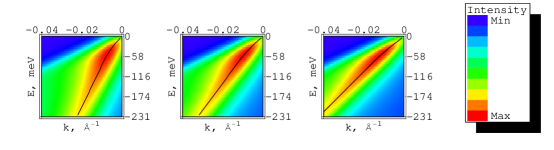
(a)  $A^{<}(k,\omega)$ at $\gamma_{\rho}=0.20$

(b)  Effective dispersion at $\gamma_{\rho}=0.20$

Figure D.1: Intensity of the spectral function $A^{<}(k,\omega)$ and effective dispersions at an interaction strength $\gamma_{\rho}=0.20$. (a) The intensity of $A^{<}(k,\omega)$ is shown for three different ratios of the spin to charge velocity, $r=0.2,~{}0.3,$ and $0.4$. The black lines are the effective electronic dispersions derived from MDC peaks, as described in the text. The dashed line in the first panel shows that the high energy part of the effective dispersion does not extrapolate back to the Fermi wavevector, $k_{F}$. (b) Comparison of the dispersions at different values of the velocity ratio, $r=0.2,~{}0.3,$ and $0.4$. In all cases the spin velocity $v_{\sigma}=0.7$eV-$\AA$ and the temperature $k_{B}T=14meV$.

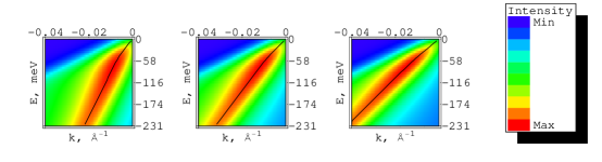
(a)  $A^{<}(k,\omega)$ at $\gamma_{\rho}=0.25$

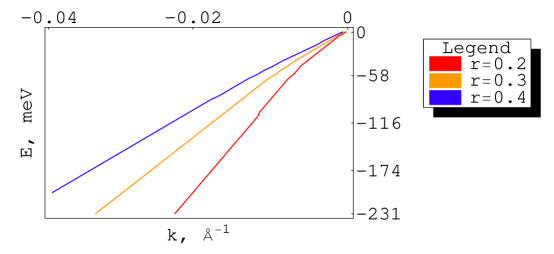
(b)  Effective dispersion at $\gamma_{\rho}=0.25$

Figure D.2: Intensity of the spectral function $A^{<}(k,\omega)$ and effective dispersions at an interaction strength $\gamma_{\rho}=0.25$. (a) The intensity of $A^{<}(k,\omega)$ is shown for three different ratios of the spin to charge velocity, $r=0.2,~{}0.3,$ and $0.4$. The black lines are the effective electronic dispersions derived from MDC peaks, as described in the text. The dashed line in the first panel shows that the high energy part of the effective dispersion does not extrapolate back to the Fermi wavevector, $k_{F}$. (b) Comparison of the dispersions at different values of the velocity ratio, $r=0.2,~{}0.3,$ and $0.4$. In all cases the spin velocity $v_{\sigma}=0.7$eV-$\AA$ and the temperature $k_{B}T=14meV$.

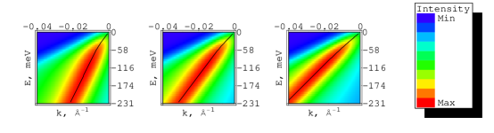
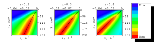
(a)  $A^{<}(k,\omega)$ at $\gamma_{\rho}=0.30$

(b)  Effective dispersion at $\gamma_{\rho}=0.30$

Figure D.3: Intensity of the spectral function $A^{<}(k,\omega)$ and effective dispersions at an interaction strength $\gamma_{\rho}=0.30$. (a) The intensity of $A^{<}(k,\omega)$ is shown for three different ratios of the spin to charge velocity, $r=0.2,~{}0.3,$ and $0.4$. The black lines are the effective electronic dispersions derived from MDC peaks, as described in the text. The dashed line in the first panel shows that the high energy part of the effective dispersion does not extrapolate back to the Fermi wavevector, $k_{F}$. (b) Comparison of the dispersions at different values of the velocity ratio, $r=0.2,~{}0.3,$ and $0.4$. In all cases the spin velocity $v_{\sigma}=0.7$eV-$\AA$ and the temperature $k_{B}T=14meV$.

(a)  $A^{<}(k,\omega)$ at $\gamma_{\rho}=0.35$

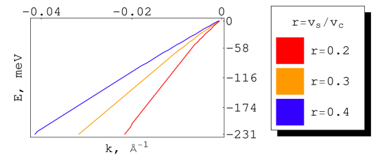
(b)  Effective dispersion at $\gamma_{\rho}=0.35$

Figure D.4: Intensity of the spectral function $A^{<}(k,\omega)$ and effective dispersions at an interaction strength $\gamma_{\rho}=0.35$. (a) The intensity of $A^{<}(k,\omega)$ is shown for three different ratios of the spin to charge velocity, $r=0.2,~{}0.3,$ and $0.4$. The black lines are the effective electronic dispersions derived from MDC peaks, as described in the text. The dashed line in the first panel shows that the high energy part of the effective dispersion does not extrapolate back to the Fermi wavevector, $k_{F}$. (b) Comparison of the dispersions at different values of the velocity ratio, $r=0.2,~{}0.3,$ and $0.4$. In all cases the spin velocity $v_{\sigma}=0.7$eV-$\AA$ and the temperature $k_{B}T=14meV$.

Trinanjan Datta was born in Calcutta (presently Kolkata), West Bengal, India. He studied at St. Xavier’s College, Calcutta and obtained his Bachelor of Science degree from the University of Calcutta in 1999 and then his Master of Science degree from the Indian Institute of Technology, Kanpur in 2001. He joined Purdue University as a doctoral candidate in the Fall of 2001. During his stay at Purdue University he held teaching assistantship positions for the initial few years. He was then awarded the Purdue Research Foundation Grant and also the Bilsland Dissertation Fellowship to complete the doctoral degree. He received his Ph.D from Purdue University in August, 2007.

References

• (1) L.D.Landau and E.M.Lifshitz. Statistical Physics, volume 5 and 9. Pergamon Press, 1980.
• (2) Aleksei A. Abrikosov, Lev. P. Gorkov, and Igor E. Dzyaloshinski. Methods of quantum field theory in statistical physics. Englewood Cliffs, N.J., Prentice-Hall, 1963.
• (3) David Pines. The theory of quantum liquids. New York, W. A. Benjamin, 1966.
• (4) G. R. Stewart. Non-fermi-liquid behavior in $d$- and $f$-electron metals. Rev. Mod. Phys., 73(4):797–855, Oct 2001.
• (5) A. M. Chang. Chiral luttinger liquids at the fractional quantum hall edge. Rev. Mod. Phys., 75(4):1449–1505, Nov 2003.
• (6) Andrea Damascelli, Zahid Hussain, and Zhi-Xun Shen. Angle-resolved photoemission studies of the cuprate superconductors. Rev. Mod. Phys., 75(2):473–541, Apr 2003.
• (7) J.T.Devreese, editor. Highly Conducting One Dimensional Solids. Plenum Press, New York, 1997.
• (8) Eduardo Fradkin. Field theories of condensed matter systems. Addision-Wesley publishing company, 1991.
• (9) Subir Sachdev. Quantum Phase Transitions. Cambridge University Press, 1999.
• (10) E. W. Carlson, V. J. Emery, S. A. Kivelson, and D. Orgad. Concepts in high temperature superconductivity. In J. Ketterson and K. Benneman, editors, The Physics of Superconductors, Vol. II. Springer-Verlag, 2004.
• (11) Neil W. Ashcroft and N. David Mermin. Solid State Physics. Harcourt College Publishers, 1976.
• (12) Assa Auerbach. Interacting electrons and quantum magnetism. Springer-Verlag, 1994.
• (13) Naoto Nagaosa. Quantum Field Theory in Condensed Matter Physics. Springer, 1999.
• (14) Naoto Nagaosa. Quantum Field Theory in Strongly Correlated Electronic Systems. Springer, 1999.
• (15) Patrick Fazekas. Lecture notes on electron correlation and magnetism. World Scientific, 1999.
• (16) Harry B. Radousky. Magnetism in heavy fermion systems. World Scientific, 2000.
• (17) A. C. Hewson. The Kondo problem to heavy fermions. Cambridge University Press, 1993.
• (18) P.Mohn. Magnetism in the Solid State, an introduction. Springer-Verlag, 2003.
• (19) L.-P.Lévy. Magnetism and Superconductivity. Springer-Verlag, 2000.
• (20) Tsuneya Ando, Alan B. Fowler, and Frank Stern. Electronic properties of two-dimensional systems. Rev. Mod. Phys., 54(2):437–672, Apr 1982.
• (21) Klaus von Klitzing. The quantized hall effect. Rev. Mod. Phys., 58(3):519–531, Jul 1986.
• (22) Horst L. Stormer, Daniel C. Tsui, and Arthur C. Gossard. The fractional quantum hall effect. Rev. Mod. Phys., 71(2):S298–S305, Mar 1999.
• (23) Shou-Cheng Zhang and Jiangping Hu. A Four-Dimensional Generalization of the Quantum Hall Effect. Science, 294(5543):823–828, 2001.
• (24) Shou-Cheng Zhang, Jiang-Ping Hu, Enrico Arrigoni, Werner Hanke, and Assa Auerbach. Projected so(5) models. Phys. Rev. B, 60(18):13070–13084, Nov 1999.
• (25) T. Giamarchi. Quantum Physics in One Dimension. Clarendon Press, Oxford, 2004.
• (26) Alexander O. Gogolin, Alexander A. Nersesyan, and Alexei M. Tsvelik. Bosonization and Strongly Correlated Systems. Cambridge University Press, 1998.
• (27) E. Miranda. Introduction to bosonization. Brazilian Journal of Physics, 33:3 – 35, 03 2003.
• (28) F D M Haldane. ’luttinger liquid theory’ of one-dimensional quantum fluids. i. properties of the luttinger model and their extension to the general 1d interacting spinless fermi gas. Journal of Physics C: Solid State Physics, 14(19):2585–2609, 1981.
• (29) S. Tomonaga. Remarks on bloch’s method of sound waves applied to many-fermion problems. Progress of Theoretical Physics, 5(4):544–569, 1950.
• (30) J. M. Luttinger. Fermi surface and some simple equilibrium properties of a system of interacting fermions. Phys. Rev., 119(4):1153–1163, Aug 1960.
• (31) Daniel C. Mattis and Elliott H. Lieb. Exact solution of a many-fermion system and its associated boson field. Journal of Mathematical Physics, 6(2):304–312, 1965.
• (32) Marc Bockrath, David H. Cobden, Paul L. McEuen, Nasreen G. Chopra, A. Zettl, Andreas Thess, and R. E. Smalley. Single-Electron Transport in Ropes of Carbon Nanotubes. Science, 275(5308):1922–1925, 1997.
• (33) F. P. Milliken, C. P. Umbach, and R. A. Webb. Indications of a luttinger liquid in the fractional quantum hall regime. Solid State Communications, 97(4):309–313, 1996.
• (34) A. M. Chang, L. N. Pfeiffer, and K. W. West. Observation of chiral luttinger behavior in electron tunneling into fractional quantum hall edges. Phys. Rev. Lett., 77(12):2538–2541, Sep 1996.
• (35) Marc Bockrath, David H. Cobden, Jia Lu, Andrew G. Rinzler, Richard E. Smalley, Leon Balents, and Paul L. McEuen. Luttinger-liquid behaviour in carbon nanotubes. Nature, 397(6720):598–601, 1999.
• (36) B. J. Kim, H. Koh, E. Rotenberg, S.-J. Oh, H. Eisaki, N. Motoyama, S. Uchida, T. Tohyama, S. Maekawa, Z.-X. Shen, and C. Kim. Distinct spinon and holon dispersions in photoemission spectral functions from one-dimensional srcuo2. Nature Physics, 2:397–401, 2006.
• (37) Dror. Orgad. Spectral functions for the tomonaga-luttinger and luther-emery liquids. Philos. Mag. B, 81(4):375, 2001.
• (38) Johannes Voit. Charge-spin separation and the spectral properties of luttinger liquids. Phys. Rev. B, 47(11):6740–6743, Mar 1993.
• (39) V. Meden and K. Scönhammer. Spectral functions for the tomonaga-luttinger model. Phys. Rev. B, 46(24):15753–15760, Dec 1992.
• (40) C. Bourbonnais and D. Jérome. Advances in Synthetic Metals, Twenty years of Progress in Science and Technology. Elsevier, 1999.
• (41) D. Jérome. Organic superconductors: From (TMTSF)2PF6 to fullerenes. Marcel Dekker, 1994.
• (42) Leon Balents and Matthew P. A. Fisher. Weak-coupling phase diagram of the two-chain hubbard model. Phys. Rev. B, 53(18):12133–12141, May 1996.
• (43) T. Giamarchi and H. J. Schulz. Correlation functions of one-dimensional quantum systems. Phys. Rev. B, 39(7):4620–4629, Mar 1989.
• (44) M. Fabrizio. Role of transverse hopping in a two-coupled-chains model. Phys. Rev. B, 48(21):15838–15860, Dec 1993.
• (45) M. Fabrizio. Role of transverse hopping in a two-coupled-chains model. Phys. Rev. B, 48(21):15838–15860, Dec 1993.
• (46) Oron Zachar. Staggered liquid phases of the one-dimensional kondo-heisenberg lattice model. Phys. Rev. B, 63(20):205104, Apr 2001.
• (47) F.V.Kusmartsev, A.Luther, and A.A.Nersesyan. Theory of a 2d luttinger liquid. JETP Lett., 55(12):724–727, 1992.
• (48) A. A. Nersesyan, A. Luther, and F. V. Kusmartsev. Scaling properties of the two-chain model. Physics Letters A, 176(5):363–370, 1993.
• (49) V.M.Yakovenko. Once again about interchain hopping. JETP Lett., 56(10):510–513, 1992.
• (50) E. Arrigoni and S. A. Kivelson. Optimal inhomogeneity for superconductivity. Phys. Rev. B, 68(18):180503, Nov 2003.
• (51) Elbio Dagotto. Experiments on ladders reveal a complex interplay between a spin-gapped normal state and superconductivity. Reports on Progress in Physics, 62(11):1525–1571, 1999.
• (52) E. Orignac and T. Giamarchi. Effects of disorder on two strongly correlated coupled chains. Phys. Rev. B, 56(12):7167–7188, Sep 1997.
• (53) A. M. Finkel’stein and A. I. Larkin. Two coupled chains with tomonaga-luttinger interactions. Phys. Rev. B, 47(16):10461–10473, Apr 1993.
• (54) Naoto Nagaosa. Bipolaron picture of spin gap state in double-chain systems. Solid State Communications, 94(7):495–498, 1995.
• (55) Takashi Kimura. Conductance renormalization and conductivity of a multisubband tomonaga-luttinger model. Phys. Rev. B, 64(23):233306, Nov 2001.
• (56) Takahashi Kimura, K Kuroki, and H Aoki. Pairing correlation in the three-leg hubbard ladder renormalization group and quantum monte carlo studies. J. Phys. Soc. Jpn, 67:1377, Sep 1997.
• (57) V. J. Emery, S. A. Kivelson, and O. Zachar. Spin-gap proximity effect mechanism of high-temperature superconductivity. Phys. Rev. B, 56(10):6120–6147, Sep 1997.
• (58) D. G. Shelton and A. M. Tsvelik. Superconductivity in a spin liquid: A one-dimensional example. Phys. Rev. B, 53(21):14036–14039, Jun 1996.
• (59) E. Dagotto, J. Riera, and D. Scalapino. Superconductivity in ladders and coupled planes. Phys. Rev. B, 45(10):5744–5747, Mar 1992.
• (60) R. M. Noack, S. R. White, and D. J. Scalapino. Correlations in a two-chain hubbard model. Phys. Rev. Lett., 73(6):882–885, Aug 1994.
• (61) D. Poilblanc, H. Tsunetsugu, and T. M. Rice. Spin gaps in coupled t-j ladders. Phys. Rev. B, 50(9):6511–6514, Sep 1994.
• (62) Hirokazu Tsunetsugu, Matthias Troyer, and T. M. Rice. Pairing and excitation spectrum in doped t-j ladders. Phys. Rev. B, 49(22):16078–16081, Jun 1994.
• (63) Steven R. White, Ian Affleck, and Douglas J. Scalapino. Friedel oscillations and charge density waves in chains and ladders. Phys. Rev. B, 65(16):165122, Apr 2002.
• (64) C. M. Varma and A. Zawadowski. Scaling in an interacting two-component (valence-fluctuation) electron gas. Phys. Rev. B, 32(11):7399–7407, Dec 1985.
• (65) W. Apel and T. M. Rice. Combined effect of disorder and interaction on the conductance of a one-dimensional fermion system. Phys. Rev. B, 26(12):7063–7065, Dec 1982.
• (66) Hsiu-Hau Lin, Leon Balents, and Matthew P. A. Fisher. Exact so(8) symmetry in the weakly-interacting two-leg ladder. Phys. Rev. B, 58(4):1794–1825, Jul 1998.
• (67) Hsiu-Hau Lin, Leon Balents, and Matthew P. A. Fisher. $n$-chain hubbard model in weak coupling. Phys. Rev. B, 56(11):6569–6593, Sep 1997.
• (68) M. Tsuchiizu and A. Furusaki. Generalized two-leg hubbard ladder at half filling: Phase diagram and quantum criticalities. Phys. Rev. B, 66(24):245106, Dec 2002.
• (69) Congjun Wu, W. Vincent Liu, and Eduardo Fradkin. Competing orders in coupled luttinger liquids. Phys. Rev. B, 68(11):115104, Sep 2003.
• (70) A. Yacoby, H. L. Stormer, Ned S. Wingreen, L. N. Pfeiffer, K. W. Baldwin, and K. W. West. Nonuniversal conductance quantization in quantum wires. Phys. Rev. Lett., 77(22):4612–4615, Nov 1996.
• (71) Loren Pfeiffer, H. L. Stormer, K. W. Baldwin, K. W. West, A. R. Goni, A. Pinczuk, R. C. Ashoori, M. M. Dignam, and W. Wegscheider. Cleaved edge overgrowth for quantum wire fabrication. Journal of Crystal Growth, 127(1-4):849–857, 1993.
• (72) J. Motohisa and H. Sakaki. Quasi-one-dimensional electron gas and its magnetic depopulation in a quantum wire prepared by overgrowth on a cleaved edge of algaas/gaas multiple quantum wells. Applied Physics Letters, 63(13):1786–1788, 1993.
• (73) C. Kurdak, A. Zaslavsky, D. C. Tsui, M. B. Santos, and M. Shayegan. High field transport in an edge overgrown lateral superlattice. Applied Physics Letters, 66(3):323–325, 1995.
• (74) Leon Balents and Matthew P. A. Fisher. Correlation effects in carbon nanotubes. Phys. Rev. B, 55(18):R11973–R11976, May 1997.
• (75) Yu. A. Krotov, D.-H. Lee, and Steven G. Louie. Low energy properties of $(n,n)$ carbon nanotubes. Phys. Rev. Lett., 78(22):4245–4248, Jun 1997.
• (76) Reinhold Egger and Alexander O. Gogolin. Effective low-energy theory for correlated carbon nanotubes. Phys. Rev. Lett., 79(25):5082–5085, Dec 1997.
• (77) Trinanjan Datta, E. W. Carlson, and Jiangping Hu. The luttinger liquid kink, 2007. arXiv.org:cond-mat/0703101.
• (78) Daniel C. Mattis. The theory of magnetism. Springer, 1988.
• (79) Patrick A. Lee, Naoto Nagaosa, and Xiao-Gang Wen. Doping a mott insulator: Physics of high-temperature superconductivity. Reviews of Modern Physics, 78(1):17, 2006.
• (80) O. M. Auslaender, H. Steinberg, A. Yacoby, Y. Tserkovnyak, B. I. Halperin, K. W. Baldwin, L. N. Pfeiffer, and K. W. West. Spin-Charge Separation and Localization in One Dimension. Science, 308(5718):88–92, 2005.
• (81) J. M. Tranquada. Neutron scattering studies of antiferromagnetic correlations in cuprates. to appear as a chapter in “Treatise of High Temperature Superconductivity” by J. Robert Schrieffer, to be published, cond-mat/0512115.
• (82) R. de Picciotto, H. L. Stormer, A. Yacoby, L. N. Pfeiffer, K. W. Baldwin, and K. W. West. Transport in cleaved-edge overgrowth wires. Physica E: Low-dimensional Systems and Nanostructures, 9(1):17–21, 2001.
• (83) A. Yacoby, H. L. Stormer, K. W. Baldwin, L. N. Pfeiffer, and K. W. West. Magneto-transport spectroscopy on a quantum wire. Solid State Communications, 101(1):77–81, 1997.
• (84) Dmitrii L. Maslov and Michael Stone. Landauer conductance of luttinger liquids with leads. Phys. Rev. B, 52(8):R5539–R5542, Aug 1995.
• (85) I. Safi and H. J. Schulz. Transport in an inhomogeneous interacting one-dimensional system. Phys. Rev. B, 52(24):R17040–R17043, Dec 1995.
• (86) V. V. Ponomarenko. Renormalization of the one-dimensional conductance in the luttinger-liquid model. Phys. Rev. B, 52(12):R8666–R8667, Sep 1995.
• (87) Dmitrii L. Maslov. Transport through dirty luttinger liquids connected to reservoirs. Phys. Rev. B, 52(20):R14368–R14371, Nov 1995.
• (88) Yaroslav Tserkovnyak, Bertrand I. Halperin, Ophir M. Auslaender, and Amir Yacoby. Finite-size effects in tunneling between parallel quantum wires. Phys. Rev. Lett., 89(13):136805, Sep 2002.
• (89) J. Moser, S. Roddaro, D. Schuh, M. Bichler, V. Pellegrini, and M. Grayson. Disordered alas wires: Temperature-dependent resonance areas within the fermi-liquid paradigm. Physical Review B (Condensed Matter and Materials Physics), 74(19):193307, 2006.
• (90) J. Moser, T. Zibold, D. Schuh, M. Bichler, F. Ertl, G. Abstreiter, M. Grayson, S. Roddaro, and V. Pellegrini. Aluminum arsenide cleaved-edge overgrown quantum wires. Applied Physics Letters, 87(5):052101, 2005.
• (91) D.Jérome and H.J.Schulz. Organic conductors and superconductors. Adv. Phys., 31:299, Aug 1982.
• (92) H. J. Schulz. Phases of two coupled luttinger liquids. Phys. Rev. B, 53(6):R2959–R2962, Feb 1996.
• (93) Roberto Casalbuoni and Giuseppe Nardulli. Inhomogeneous superconductivity in condensed matter and qcd. Reviews of Modern Physics, 76(1):263, 2004.
• (94) E. W. Carlson, D. Orgad, S. A. Kivelson, and V. J. Emery. Dimensional crossover in quasi-one-dimensional and high-t[sub c] superconductors. Physical Review B (Condensed Matter and Materials Physics), 62(5):3422–3437, 2000.
• (95) R. Claessen, G.-H. Gweon, F. Reinert, J. W. Allen, W. P. Ellis, Z.-X. Shen, C. G. Olson, L. F. Schneemeyer, and F. L vy. Angle-resolved photoemission of quasi-one-dimensional metals: Evidence for luttinger liquid behavior. J. Elect. Spect. Rel. Phenom., 76:121–126, 1995.
• (96) P. Segovia, D. Purdie, M. Hengsberger, and Y. Baer. Observation of spin and charge collective modes in one-dimensional metallic chains. Nature, 402:504–507, 1999.
• (97) José-Luis Mozos, Pablo Ordejón, and Enric Canadell. First-principles study of the blue bronze $k_{0.3}moo_{3}$. Phys. Rev. B, 65(23):233105, Jun 2002.
• (98) R. Losio, K. N. Altmann, A. Kirakosian, J.-L. Lin, D. Y. Petrovykh, and F. J. Himpsel. Band splitting for si(557)-au: Is it spin-charge separation? Phys. Rev. Lett., 86(20):4632–4635, May 2001.
• (99) R. Claessen, M. Sing, U. Schwingenschlögl, P. Blaha, M. Dressel, and C. S. Jacobsen. Spectroscopic signatures of spin-charge separation in the quasi-one-dimensional organic conductor ttf-tcnq. Phys. Rev. Lett., 88(9):096402, Feb 2002.
• (100) Jhinhwan Lee, S. Eggert, H. Kim, S.-J. Kahng, H. Shinohara, and Y. Kuk. Real space imaging of one-dimensional standing waves: Direct evidence for a luttinger liquid. Physical Review Letters, 93(16):166403, 2004.
• (101) G.Morandi, P.Sodano, A.Tagliacozzo, and V.Tognetti, editors. Field theories for low-dimensional condensed matter systems (spin systems and strongly correlated electrons). Springer-Verlag, 2000.
• (102) J Voit. One-dimensional fermi liquids. Reports on Progress in Physics, 58(9):977–1116, 1995.
• (103) D. Senechal. An introduction to bosonization, 1999.
• (104) Nigel Goldenfeld. Lectures on Phase Transitions and the Renormalization Group. Perseus Publishing, 1992.
• (105) Shang-Keng Ma. Statistical Mechanics. World Scientific, 1985.
• (106) Kenneth G. Wilson and J. Kogut. The renormalization group and the [epsilon] expansion. Physics Reports, 12(2):75–199, 1974.
• (107) Michel Le Bellac. Quantum and Statistical Field Theory. Oxford Science Publications, 1991.
• (108) Zinn-Justin. Quantum Field Theory and Critical Phenomena. Oxford Science Publications, 1991.
• (109) P. M. Chaikin and T.C. Lubensky. Principles of Condensed Matter Physics. Cambridge University Press, 1995.
• (110) Oleg A. Starykh, Dmitrii L. Maslov, Wolfgang Hausler, and Leonid I. Glazman. Interactions and Quantum Transport Properties of Lower Dimensional Systems, Lecture Notes in Physics,. Springer, 2000.
• (111) C. L. Kane and Matthew P. A. Fisher. Transport in a one-channel luttinger liquid. Phys. Rev. Lett., 68(8):1220–1223, Feb 1992.
• (112) C. L. Kane and Matthew P. A. Fisher. Transmission through barriers and resonant tunneling in an interacting one-dimensional electron gas. Phys. Rev. B, 46(23):15233–15262, Dec 1992.
• (113) M. Shayegan, E. P. De Poortere, O. Gunawan, Y. P. Shkolnikov, E. Tutuc, and K. Vakili. Two-dimensional electrons occupying multiple valleys in alas, 2006. arXiv.org:cond-mat/0606158.
• (114) Y. P. Shkolnikov, E. P. De Poortere, E. Tutuc, and M. Shayegan. Valley splitting of alas two-dimensional electrons in a perpendicular magnetic field. Phys. Rev. Lett., 89(22):226805, Nov 2002.
• (115) Private communications with Dr. Yen Lee Loh.
• (116) O. Gunawan, Y. P. Shkolnikov, E. P. De Poortere, E. Tutuc, and M. Shayegan. Ballistic electron transport in alas quantum wells. Physical Review Letters, 93(24):246603, 2004.
• (117) D. Orgad, S. A. Kivelson, E. W. Carlson, V. J. Emery, X. J. Zhou, and Z. X. Shen. Evidence of electron fractionalization from photoemission spectra in the high temperature superconductors. Phys. Rev. Lett., 86(19):4362–4365, May 2001.
• (118) H.J.Schulz. Fermi liquids and non-fermi liquids. In E. Akkermans, G.Montambaux, J.L.Pichard, and J.Zinn-Justin, editors, Mesoscopic Quantum Physics, Les Houches LXI. Amsterdam, Elsevier, 1995.
\coversheet
APPENDICES \@@nonchapteroddAPPENDICESy0pt