Phase Transitions and Computational Difficulty in Random Constraint Satisfaction Problems

Abstract

We review the understanding of the random constraint satisfaction problems, focusing on the $q$-coloring of large random graphs, that has been achieved using the cavity method. We also discuss the properties of the phase diagram in temperature, the connections with the glass transition phenomenology in physics, and the related algorithmic issues.

1 Introduction

Spin glass theory has a large and probably initially unexpected impact on some problems far from condensed matter physics and one example of such spectacular outcome is the application of statistical physics ideas to combinatorial optimization [1] and of the concept of phase transitions to the probabilistic analysis of Constraint Satisfaction Problems (CSPs) [2, 3, 4]. Given a set of $N$ discrete variables subject to a set of $M$ constraints, a CSP consists in deciding if there exists an assignment of the variables satisfying all the constraints. This is a generic setting that is currently used to tackle problems as diverse as, among others, error-correcting codes, register allocation in compilers or genetic regulatory networks. The class of NP-complete problems [1], for which no algorithm is known that guarantees to decide satisfiability in a time polynomial in $N$, is particularly interesting. Well-studied examples of such problems are the satisfiability of boolean formulas (SAT), and the $q$-coloring problem ($q$-COL, see figure 1) that we shall discuss here. Given a graph with $N$ vertices and $M$ edges connecting certain pairs of them, and given $q$ colors, can we color the vertices so that no two connected vertices have the same color?

Crucial empirical observations were made when considering the ensemble of random graphs with a given average vertex connectivity $c$: while below a critical value $c_{s}$ a proper $q$-coloring of the graph exists with a probability going to one in the large size limit, it was found that beyond $c_{s}$ no proper $q$-coloring exists asymptotically. This sharp threshold (which appears in other CSPs such as K-SAT and whose existence is partially proved in [5]) is an example of a phase transition arising in random CSPs. It was also observed empirically [6, 7] that deciding colorability becomes on average much harder near to the coloring threshold $c_{s}$ than far away from it. It is therefore natural to ask ourselves: Can the value of the colorable/uncolorable (COL/UNCOL) phase transition be computed? Can the number of all possible colorings be also computed? Are there other interesting phase transitions? Can these transitions explain the fact that solutions are sometimes very hard to find? Can this knowledge help us in designing new algorithms? These questions, and their answers, are at the roots of the interest of the statistical physics community in optimization problems [3, 4].

2 A Potts anti-ferromagnet on random graphs

It is immediate to realize that the $q$-coloring problem is equivalent to the question of determining if the ground-state energy of a Potts anti-ferromagnet on a random graph is zero or not [8]. Consider indeed a graph $G=({\cal V,E})$ defined by its vertices ${\cal V}=\{1,\dots,N\}$ and edges $(i,j)\in{\cal E}$ which connect pairs of vertices $i,j\in{\cal V}$; and the Hamiltonian

$${\cal H}(\{s\})=\sum_{(i,j)\in{\cal E}}\delta(s_{i},s_{j})\,.$$ (1)

With this choice there is no energy contribution for neighbors with different colors, but a positive contribution otherwise. The ground state energy (the energy at zero temperature) is thus zero if and only if the graph is $q$-colorable. This transforms the coloring problem into a well-defined statistical physics model. Usually, two types of random graphs are considered: in the $c-$regular ensemble all points are connected to exactly $c$ neighbors, while in the Erdős-Rényi case the connectivity has a Poisson distribution.

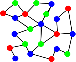
Figure 1: Example: a proper 3-coloring of a small graph.

3 Cavity method: Warnings, Beliefs and Surveys

Over the last few years, a number of studies have investigated CSPs following the adaptation of the so-called cavity method [2] to random graphs [4, 9]. It is a powerful heuristic tool —whose exactness is widely accepted but has still to be rigorously demonstrated— equivalent to the replica method of disordered systems [2]. Its main idea lies in the fact that a large random graph is locally tree-like, and that an iterative procedure known in physics as the Bethe-Peirls method can solve exactly any model on a tree (such models are often qualified as “mean field” in physics). Interestingly, it was realized [10] that an equivalent formalism has been developed independently in computer science [11], where it is called Belief Propagation (BP, which conveniently enough, may also stands for Bethe-Peirls). Defining $\psi^{i\to j}_{c}(c=1,..,q)$ as the probability that the spin $i$ has color $c$ in absence of the spin $j$ (the “belief” that the spin $j$ has on the properties of the spin $i$), BP reads

$$\psi_{c}^{i\to j}=\frac{1}{Z_{0}^{i\to j}}\prod_{k\in N(i)\setminus\{j\}}\left(1-\psi_{c}^{k\to i}\right)$$ (2)

where $Z_{0}^{i\to j}$ is a normalization constant and the notation $k\in N(i)\setminus\{j\}$ means the set of neighbors of $i$ except $j$. From a fixed point of these equations, the complete beliefs in presence of all spins can be also computed. They give, for each vertex, the probability of each color from which other quantities, as for instance the number of solutions, can be computed. A simpler formalism, called Warning Propagation (WP), restricts itself to frozen variables (i.e. to variables for which only one color can satisfy the constraints). However, WP does not allow to compute the number of solutions, only their existence, but is definitely simpler to handle.

It was soon realized, however, that these methods developed for trees could not be used straightforwardly on all random graphs because of a non-trivial phenomenon called clustering [9, 12] (for which rigorous results are now available, see [13]). Indeed, while for graphs with very low connectivities all solutions are “connected” —in the sense that it is easy with a local dynamics to move from one solution to another— they regroup into a large number of disconnected clusters for larger connectivities. It can be argued that each of these clusters corresponds to a different fixed point of the BP equations, so that a survey over the whole set of the fixed points should be performed. This can be done in the cavity method by the now famous Survey Propagation (SP) equations [4] which, in the physics language, correspond to the Parisi’s one-step Replica Symmetry Breaking (RSB) scheme [2]. Within this formalism, the number of clusters (which behaves as ${\cal{N}}=e^{N\Sigma}$, where $\Sigma$ is a fundamental quantity called the complexity) and their sizes (the number of proper colorings inside the cluster) can be determined.

This formalism has been applied on the SAT [4] and COL [14, 15] problems in the limit of infinitely large graphs. These cutting edge studies were however restricted to SP applied to the clusters corresponding to fixed points of WP and not to those of BP. Although this already allowed the correct computation of the COL/UNCOL transition and the development of a powerful algorithm [4], it meant that the description of the clustered phase was only partial and this resulted in a number of problems and inconsistencies that stayed unanswered until very recently. These issues have been today clarified [16, 17, 18, 19, 20, 21] and we shall now discuss this new understanding.

4 The phase diagram of the coloring problem on a random graph

Consider that we have $q\geq 4$ colors (the $q=3$ case being a bit particular [16, 18, 20], as we shall see) and a large random graph whose connectivity $c$ we shall increase. Different phases are encountered that we will now describe (and enumerate) in order of appearance (the corresponding phase diagram is depicted in figure 2).

• A unique cluster exists: For low enough connectivities, all the proper colorings are found in a single cluster, where it is easy to “move” from one solution to another. Only one possible —and trivial— fixed point of the BP equations exists at this stage (as can be proved rigorously in some cases [23]). The entropy can be computed and reads in the large graph size $N$ limit

  $$s=\frac{\log{\cal{N}}_{\rm sol}}{N}=\log{q}+\frac{c}{2}\log{\left(1-\frac{1}{q}\right)}\,.$$ (3)

• Some (irrelevant) clusters appear: As the connectivity is slightly increased, the phase space of solutions decomposes into an large (exponential) number of different clusters. It is tempting to identify that as the clustering transition, but it happens that all (but one) of these clusters contain relatively very few solutions —as compare to whole set— and that almost all proper colorings still belong to one single giant cluster. Clearly, this is not a proper clustering phenomenon and in fact, for all practical purpose, there is still only one single cluster. equation (3) still gives the correct entropy at this stage.

• The clustered phase: For larger connectivities, the large single cluster also decomposes into an exponential number of smaller ones: this now defines the genuine clustering threshold $c_{d}$. Beyond this threshold, a local algorithm that tries to move in the space of solutions will remain prisoner of a cluster of solutions [24]. Interestingly, it can be shown that the total number of solutions is still given by equation (3) in this phase. This is because, as is well known in the replica method, the free energy has no singularity at the dynamical transition (which is therefore not a true transition in the sense of Ehrenfest, but rather a dynamical or geometrical transition in the space of solutions).

• The condensed phase: As the connectivity is further increased, a new sharp phase transition arises at the condensation threshold $c_{c}$ where most of the solutions are found in a finite number of the largest clusters. From this point, equation (3) is not valid anymore and becomes just an upper bound. The entropy is non-analytic at $c_{c}$ therefore this is a genuine static phase transition.

• The rigid phase: As mentioned in section 3, two different types of clusters exist: In the first type, that we shall call the unfrozen ones, all spins can take at least two different colors. In the second type, however, a finite fraction of spins is allowed only one color within the cluster and are thus “frozen” into this color. These frozen clusters actually correspond to non-trivial fixed points of BP and WP, while the first kind are non-trivial fixed points of BP only. It follows that a transition exists, that we call rigidity, when frozen variables appear inside the dominant clusters (those that contains most colorings). If one takes a proper coloring at random beyond $c_{r}$, it will belong to a cluster where a finite fraction of variables is frozen into the same color. Depending on the value of $q$, this transition may arise before or after the condensation transition (see table 1).

• The UNCOL phase: Eventually, the connectivity $c_{s}$ is reached beyond which no more solutions exist. The ground state energy (sketched in figure 3) is zero for $c<c_{s}$ and then grows continuously for $c>c_{s}$. The values $c_{s}$ computed within the cavity formalism are in perfect agreement with the rigorous bounds [25] derived using probabilistic methods and are widely believed to be exact (although they remains to be rigorously proven, but see [26] for a proof that they are at least rigorous upper bounds).

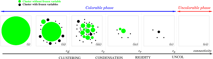
Figure 2: Sketch of the space of solutions —colored points in this representation— in the $q$-coloring problem on random graphs when the connectivity $c$ is increased. (i) At low $c$, all solutions belong to a single cluster. (ii) For larger $c$, other clusters of solutions appear but a giant cluster still contains almost all solutions. (iii) At the clustering transition $c_{d}$, it splits into an exponentially large number of clusters. (iv) At the condensation transition $c_{c}$, most colorings are found in the few largest of them. (v) The rigidity transition $c_{r}$ ($c_{r}<c_{c}$ and $c_{r}>c_{c}$ are both possible depending on $q$) arises when typical solutions belong to clusters with frozen variables (that are allowed only one color in the cluster). (vi) No proper coloring exists beyond the COL/UNCOL threshold $c_{s}$.

We report the values of the threshold connectivities corresponding to all these transitions in table 1 for the regular and the Poissonian (i.e. Erdős-Rényi) random graphs ensembles. Notice that the $3$-coloring is peculiar because $c_{d}=c_{c}$ so that the clustered phase is always condensed in this case. In view of this rich phase diagram, it is important to get an intuition on the meaning and the properties of these different phases and, in this respect, it is interesting before entering the algorithmic implications to discuss the analogies with the glass transition.

q	$c_{d}$	$c_{r}$	$c_{c}$	$c_{s}$
3	$5^{+}$	-	6	6
4	9	-	10	10
5	14	14	14	15
6	18	19	19	20
7	23	-	25	25
8	29	30	31	31
9	34	36	37	37
10	39	42	43	44

q	$c_{d}$	$c_{r}$	$c_{c}$	$c_{s}$
3	4	4.66(1)	4	4.687(2)
4	8.353(3)	8.83(2)	8.46(1)	8.901(2)
5	12.837(3)	13.55(2)	13.23(1)	13.669(2)
6	17.645(5)	18.68(2)	18.44(1)	18.880(2)
7	22.705(5)	24.16(2)	24.01(1)	24.455(5)
8	27.95(5)	29.93(3)	29.90(1)	30.335(5)
9	33.45(5)	35.658	36.08(5)	36.490(5)
10	39.0(1)	41.508	42.50(5)	42.93(1)

Table 1: Threshold connectivities $c_{d}$ (dynamical/clustering) [20, 17, 18, 27], $c_{r}$ (rigidity/freezing) [20, 21], $c_{c}$ (condensation/Kauzmann) [20, 18] and $c_{s}$ (COL/UNCOL) [14, 15] for regular (left) and Erdős-Rényi (right) random graphs. In the large $q$-limit, one finds in both cases that [20, 18]: $c_{r}=q[\log q+\log\log q+1+o(1)]$, $c_{c}=2q\log{q}-\log{q}-2\log{2}+o(1)$ and [15]: $c_{s}=2q\log{q}-\log{q}-1+o(1)$.

5 A detour into the ideal glass transition phenomenology

To those familiar with the replica theory and the mean field theory of glasses, the phenomenology depicted in the former section should look familiar: these successive transitions are indeed very well known in the picture of the ideal glass transition [28]. This striking analogy is in fact quite natural since, despite the fact that there is no disorder in the interactions in Hamiltonian (1), the frustration due to the loops in the random graph makes the model behaving like a disordered “anti-ferromagnetic” Potts spin glass [29] and such models are known to display the glassy phenomenology [8, 28].

The phase diagram obtained on Poissonian random graphs with average connectivity $c$ for $q\geq 4$ is sketched in figure 3 (the $q=3$ model is slightly different as, again, $T_{d}=T_{c}$). At high temperature the system behaves as a liquid (or a paramagnet in the language of magnetic systems). Below a temperature $T_{d}$ a first transition —called “dynamical”— happens and the system falls out of equilibrium. For $T<T_{d}$ it is not possible for a physical dynamics to equilibrate the system and the ergodicity is broken: this is due to the appearance of exponentially many different states. However, the would-be equilibrium properties of the problem remain similar (and in particular, the free-energy has no singularity at this temperature). Only at temperature $T_{c}$ the free energy is non analytic and a true “static” glass transition happens, called the Kauzmann transition [28]. In this phase only a finite number of states does matter at a given connectivity. Finally, for larger connectivities, a third phenomenon is observed as the temperature is further lowered, called the Gardner transition [30, 31]. It is a transition towards a more complicated phase, similar to the one found in the celebrated solution of the Sherrington-Kirkpatrick model [2]. The fact that the Gardner transition arises for connectivities larger the COL/UNCOL one is very important in this respect: it shows that the study of this phase, that requires a more involved cavity formalism (and probably further RSB), does not seem to be needed in the colorable phase. We also now recognize that the “clustering” and the “condensation” transitions in the coloring problem are just the zero temperature relics of the dynamic and Kauzmann transitions at finite temperatures.

A similar connection with the physics of glassy system can also be obtained directly at zero temperature via the jamming phenomenology [19] where the density of constraints (in this case the volume of some non-overlapping spheres in a box of fixed volume) are increased and where a dynamical transition is first met while some authorized configurations exist much beyond this point (see for instance [33] and references therein).

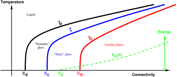
Figure 3: Sketch of the phase diagram in the coloring problem at finite temperature (from [29]). At $T_{d}$, the system falls out of equilibrium (“dynamic” transition). At $T_{c}$ the system undergoes a “static” glass transition. Finally, at $T_{G}$, a Gardner transition appears. $e_{GS}$ represents the ground state energy.

We thus see that the coloring problem on random graphs translates into a very general mean field model of a complex liquid. This convergence of interest between different disciplines is quite interesting in itself and allows to discuss a number of matters, as we shall now see.

6 Onset of hardness for local search algorithms

The properties of the phase diagram we just discussed are based on analytical computations through the cavity method. We would like to discuss now what are the implications of these different phases on the performance of simple local search algorithms that try to find a solution. This is, however, a much harder subject to handle analytically and we shall thus leave the field of analytical computations to enter the one of phenomenology. Still, the behavior of an algorithm trying to find a solution is reminiscent of the behavior of the physical dynamics in glassy systems, and we can at least exploit this analogy in order to get an intuition for the problem that we can later confirm with numerical simulations.

It is first tempting to identify the point $c_{d}$, where a physical Monte-Carlo dynamics gets trapped into a cluster, with the onset of computational hardness. However, a second moment though indicates that this should not be the case: In the glass transition phenomenology, it is well known that, although the system falls out of equilibrium beyond $T_{d}$, its energy can be further lowered by lowering the temperature, or just by waiting a bit longer [19]. In short: the fact that dynamics is prisoner of a given region of the set of possible configurations does not mean that no solution can be found in this region. Although $c_{d}$ is indeed a sharp transition for the Monte-Carlo sampling, there is no reason, a priori, to experience difficulties if one just want to find one solution beyond this point. This is particularly transparent in the analysis and the algorithm introduced in [19] (and directly inspired from the analogy with jamming [33]):

1. Start with a graph of connectivity $c$ and a proper coloring.

2. Increase the density of constraint by adding a link in the graph.

3. Use a simple algorithm in order to solve the contradiction introduced by the link. When it is done, go back to step (i).

By applying this strategy, starting from scratch (i.e. from a graph with $N$ vertices and no link), the set of all proper colorings undergoes the successive transitions described in figure 2 as connectivity increases. When the dynamical transition is reached, one is trapped inside a cluster of solutions, but this is not really a problem as one is still free to move inside the cluster. As more links are added, the cluster size is decreasing continuously but while it still exists, the local algorithm should be in principle able to find solutions nearby. Only for larger connectivities, when the cluster gets frozen, it disappears and consequently the algorithm stops. It was shown in Ref. [19] through numerical simulations that this strategy, using the Walk-COL [20] algorithm for step (iii), is indeed efficient, and linear in $N$, much beyond the dynamical transition.

The reason why this recursive strategy becomes inefficient when the cluster in which the dynamics is trapped freezes is the following: if a link is put between two vertices frozen in the same color, it is impossible to satisfy the constraints while remaining in the cluster. As opposed to the unfrozen clusters, the frozen clusters thus have a finite probability to disappear when a new link is added. A cavity-like analysis [21], confirmed by numerical data [19], actually shows that the number of changes that the algorithm must perform, in order to solve the contradictions imposed by the addition of new links, increases with the connectivity and diverges when the frozen variables appear. The source of difficulties is therefore not the clustering phenomenon in itself, but rather the appearance of frozen variables. This makes the analysis and the prediction of a EASY/HARD threshold much harder since (as one can see on figure 2) clusters of different sizes freeze at different connectivities, although a connectivity $c_{*}\geq c_{r}$ exists where all clusters are frozen, thus putting a strict bound to the efficiency of this procedure.

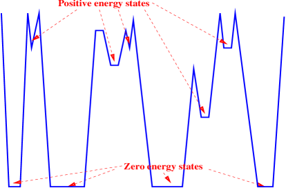
Figure 4: Artist’s view of the energy landscape for low connectivities $c>c_{d}$: a region dominated by canyons that reach the ground-states.

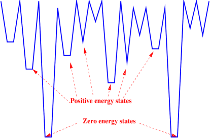
Figure 5: Artist’s view of the energy landscape for large connectivities $c>c_{d}$: a region dominated by high mountains and deep valleys.

Interestingly, even non-incremental algorithms may also pass the $c_{d}$ threshold [34, 20], and that might come as a surprise for those having in mind the “rugged” many-valley energy landscape picture of spin glasses. This apparent paradox can be clarified by the following considerations: It is possible that at lower connectivity $c>c_{d}$ the energy landscape is dominated by deep canyons (figure 5), where it is in principle easy to go down as one has just to jump ahead! At larger connectivities a more rugged region with many deep valleys and high mountains is found (figure 5) in which case, as any mountain-hiker will undoubtly know, it takes some time to go to the deepest valley because many hills have to be climbed first. This difference in behavior might explain the “unreasonable efficiency” of local algorithm [7] and the performance of the annealing procedure beyond $c_{d}$ [27].

To further illustrate this point, consider the Walk-COL algorithm introduced in [20] (and adapted from a similar one in SAT [34]) defined by the following procedure

1. Randomly choose a spin that has the same color as at least one of its neighbors.

2. Change randomly its color. Accept this change with probability one if the number of unsatisfied spins has been lowered, otherwise accept it with probability $p$ (this is a parameter that has to be tuned for better efficiency).

3. If there are unsatisfied vertices, go to step (i) unless the maximum running time is reached.

This algorithm can easily find colorings for large sizes in linear time beyond $c_{d}$ [20], but certainly not too close to the UNCOL transition where it gets trapped at higher energies (see figure 6).

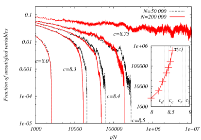
Figure 6: Fraction of unsatisfied variables versus the number of attempted flips of the Walk-COL algorithm divided by the size of the graph in the $q=4$ coloring: Walk-COL [20] algorithm is able to find some solutions in the clustered phase for low $c$ (in the canyon-like region), but get trapped in the high energy valleys for larger $c$. Inset: estimated time $\tau=t/N$ needed to find a solution versus connectivity.

So far, there are few analytical results about the energy landscape in this problem and it is likely that this will be the subject of further studies. It is unfortunately very hard to say for which connectivities the landscape goes from canyons-dominated to mountains-dominated as this may not be a sharp transition and more a matter of —certainly algorithm-dependent— basins of attraction. The rigidity transition for typical clusters is certainly a good candidate as a crossover in behavior (as is the connectivity where all clusters are frozen).

To conclude, one sees that although the algorithmic issues are indeed more difficult to handle than the phase diagram, at least two important points can already be made: First, the dynamical transition does not correspond to the onset of hardness, and second, the source of difficulty seems more to be related with the appearance of frozen variables.

7 Message Passing and Decimation

The class of local search algorithms is only one part of the story. A different class, where messages are exchanged through the nodes of the graph, was proven to be very efficient in computer science. BP and WP are examples of such procedures and it is thus interesting to use the information given by the cavity analysis to discuss their performance in estimating the marginals —or other informations— in the problem. A major outcome of the last years has also been the application of SP as a message passing (MP) [4].

From the information given by the fixed point of the MP, an algorithm can be defined in the following way [4]: (i) run the MP to obtain some information, and (ii) fix (decimate) some variables according to this information. This sequence is iterated until a solution is found, or until a contradiction is met. The two parts are quite independent and each of them can be changed separately (for instance a self consistent re-enforcement has been tried instead of the decimation with very good results [35]).

According to the cavity formalism, the iterative fixed point of BP correctly estimates the marginals until the condensation at $c_{c}$ [18] (which, conveniently, is very close to $c_{s}$). Indeed the application of BP plus decimation is numerically efficient in finding solutions for both SAT and COL [18, 20, 22] and it would be interesting to see if this method allows to find “typical” solutions beyond $c_{d}$, thus bypassing the problems of Monte-Carlo algorithms. It seems that the strategy is efficient even beyond $c_{c}$ in some cases [20], although the BP recursion does not always converge (and when it does, it does it slowly) on the decimated graph, in which case an imprecise and approximate information is obtained. These issues are thus far from being properly understood at the present time, and we hope that new works will be done in this direction.

A more powerful strategy in the clustered phase is to use SP to compute the probability that a given variable is frozen is a cluster [4]. Fixing the variables which are frozen in most clusters seems a good way to decimate the graph. Using this method in random 3-SAT allows to outperform any other known algorithm and to find solutions of huge instances rapidly even very close to the threshold [4, 35]. The method has been subsequently adapted for the $3-$coloring in [14]. Interestingly, SP behaves better than BP on the decimated graph and has no problem of convergence. Other strategies are possible that have not yet been exploited [20].

The best way to extract the informations given by the fixed point of these message passing procedures is however not yet known, nor is the limit until where these strategies are efficient. However, this line of thoughts is certainly the most promising way in the direction of better solving and sampling algorithms.

8 Conclusions and perspectives

In this paper, we considered and reviewed some aspects of the $q-$coloring of large random graphs. We discussed the properties of the set of solutions and the different sharp phase transitions it undergoes when the average connectivity is varied. The problem translates in physics into a mean-field model with an ideal glass transition. The cavity method has been efficient in giving insight into the problem, although the important challenge of proving rigorously these results remains. It would be interesting in this respect to confirm these predictions by performing extensive Monte-Carlo simulations of the phase diagram depicted in figure 3.

We also discussed the dynamical behavior of local search algorithms. We saw that although the “dynamical” transition has a direct meaning as the point where local Monte-Carlo algorithms get out of equilibrium, it is not directly connected with the onset of hardness in the problem which is rather due to the fact that clusters “freeze” as the connectivity increases. So far, it has not therefore been possible, despite initial hope, to have well-defined HARD and EASY phases. The precise role of frozen variables and the part played by the rigidity transition, or by the connectivity where all clusters becomes frozen, will undoubtly be the subject of new research, both in numerical and theoretical directions, that will help to clarify these issues. A refined knowledge of the energy landscape would also be valuable.

Finally, we also discuss the major breakthrough in the algorithmic strategy that emerged from the application of the cavity solution on a single given graph. It is not clear at the present time what it the best way to use this approach and how efficient it can be, nor if it is possible to go arbitrarily close to the satisfiability/colorability threshold for any values of $q$, and it is likely that these questions will also trigger a lot of work in the future.

We thank J. Kurchan, A. Montanari, F. Ricci-Tersenghi and G. Semerjian for the collaborations that led to a substantial part of our results. We also greatly benefit from discussions with M. Mézard and R. Zecchina. We thank T. Jörg and A. Hartmann for a critical lecture of the paper.

References

References

- [1] Cook S 1971 Proc. of the 3rd Annual ACM Symp. on Theory of Computing (ACM, New York) pp. 151-158. Papadimitrious C H 1994 Computational Complexity (Addison-Wesley, Reading, MA). Garey M R and Johnson D S 1979 Computers and Intractability (Freeman, San Francisco). Dubois O, Monasson R, Selman B, and Zecchina R 2001 special issue of Theor. Comp. Sci. 265. Hartmann A K and Weigt M 2005 Phase Transitions in Combinatorial Optimization Problems (Wiley-VCH, Berlin).
- [2] Mézard M, Parisi G and Virasoro M A 1997 Spin-glass Theory and Beyond (Singapore: World Scientific).
- [3] Monasson R, Zecchina R, Kirkpatrick S, Selman B and Troyansky L 1999 Nature 400 133.
- [4] Mézard M, Parisi G and Zecchina R 2002 Science 297 812. Mézard M and Zecchina R 2002 Phys. Rev. E 66 056126. Braunstein A, Mézard M, and Zecchina R 2005 Random Struct. Algorithms 27 201.
- [5] Friedgut E and Bourgain J 1999 Journal of the American Mathematical Society 12 4. Achlioptas D and Friedgut E 1999 Random Struct. Algorithms 14 1.
- [6] Cheeseman P, Kanefsky B and Waylor W M 1991 Proc. of the Twelfth Int. Joint Conf. on Artificial Intelligence (Sydney, Australia).
- [7] Selman B and Kirkpatrick S 1996 Artif. Intell. 81 273. Selman B, Mitchell D G, and Levesque H J 1996 ibid. 81 17.
- [8] Kanter I et Sompolinsky H 1987 J. Phys. A: Math. Gen. 20 L673. Gross D J, Kanter I and Sompolinsky H 1985 Phys. Rev. Lett. 55 304.
- [9] Mézard M and Parisi G 2001 Eur. Phys. J. B 20 217 and 2003 J. Stat. Phys 111 1-2 1.
- [10] Yedidia J S, Freeman W T and Weiss Y 2003 Exploring Artificial Intelligence in the New Millennium ISBN 1558608117, Chap. 8, pp. 239-236 (Science and Technology Books).
- [11] Pearl J 1988 Probabilistic Reasoning in Intelligent Systems: Networks of Plausible Inference (2nd edition, Morgan Kaufmann Publishers, San Francisco).
- [12] Biroli G, Monasson R and Weigt M 2000 Eur. Phys. J. B 14 551.
- [13] Mézard M, Mora T and Zecchina R 2005 Phys. Rev. Lett. 94 197205. Achlioptas D and Ricci-Tersenghi F 2007 Proc. of the annual ACM Symp. on Theory of computing (Seattle WA).
- [14] Mulet R, Pagnani A, Weigt M and Zecchina R 2002 Phys. Rev. Lett. 89 268701. Braunstein A, Mulet R, Pagnani A, Weigt M and Zecchina R 2003, Phys. Rev. E 68 036702.
- [15] Krzakala F, Pagnani A and Weigt M 2004 Phys. Rev. E 70 046705.
- [16] Mézard M, Palassini M and Rivoire O 2005 Phys. Rev. Lett. 95 200202.
- [17] Mézard M and Montanari A 2006 J. Stat. Phys. 124 1317.
- [18] Krzakala F, Montanari A, Ricci-Tersenghi F, Semerjian G and Zdeborová L 2007 Proc. Natl. Acad. Sci. 104 10318.
- [19] Krzakala F and Kurchan J 2007 Phys. Rev. E 76 021122.
- [20] Zdeborová L and Krzakala F 2007 Phys. Rev. E 76 031131.
- [21] Semerjian G 2007 On the freezing of variables in random constraint satisfaction problems Preprint arXiv:0705.2147 (J. Stat. Phys., on press).
- [22] Montanari A, Ricci-Tersenghi F, Semerjian F 2007 Solving Constraint Satisfaction Problems through Belief Propagation-guided decimation Preprint arXiv:0709.1667.
- [23] Bandyopadhyay A and Gamarnik D 2006 ACM-SIAM Symp. on Discrete Algorithms 890. Jonasson J 2002 Statistics and Probability Letters 57 243.
- [24] Montanari A and Semerjian G 2006 J. Stat. Phys. 124 103.
- [25] Luczak T 1991 Combinatorica 11 45. Achlioptas D, Naor A and Peres Y 2005 Nature 435 759.
- [26] Franz S and Leone M 2003 J. Stat. Phys. 111 535.
- [27] van Mourik J and Saad D 2002 Phys. Rev. E 66 056120.
- [28] Gross D J and Mézard M 1984 Nuclear Physics B 240 4 431. Kirkpatrick T, Thirumalai D, and Wolynes P 1989 Phys. Rev. A 40 1045. Mézard M and Parisi G 1999 Phys. Rev. Lett. 82 747.
- [29] Krzakala F and Zdeborová L 2007 Potts Glass on Random Graphs Preprint arXiv:0710.3336.
- [30] Gardner E 1985 Nuclear Physics B 257 747.
- [31] Leuzzi L and Parisi G 2001 J. Stat. Phys. 103 679. Crisanti A, Leuzzi L and Parisi G 2002 J. Phys. A: Math. Gen. 35 481.
- [32] Montanari A, Parisi G and Ricci-Tersenghi F 2004 J. Phys. A: Math. Gen. 37 2073. Mertens S, Mézard M and Zecchina R 2003 Random Struct. Algorithms 28 3 340.
- [33] Liu A and Nagel S 1998 Nature 396 21. O’Hern C S, Silbert L E, Liu A and Nagel S 2003 Phys. Rev. E 68 011306. Wyart M 2005 Annales de Physique 30 3.
- [34] Ardelius J and Aurell E 2006 Phys. Rev. E 74 037702.
- [35] Chavas J, Furtlehner C, Mézard M, and Zecchina R 2005 J. Stat. Mech. P11016.