Erratum to Star formation triggered by SN explosions: an application to the stellar association of $\beta$Pictoris

Abstract

This is an erratum to the article entitled ”Star formation triggered by SN explosions: an application to the stellar association of $\beta$ Pictoris” by C. Melioli, E. M. de Gouveia Dal Pino, R. de la Reza and A. Raga which was published in this Journal (MNRAS, 373, 811-818, 2006) with the following original abstract:

In the present study, considering the physical conditions that are relevant interactions between supernova remnants (SNRs) and dense molecular clouds for triggering star formation we have built a diagram of SNR radius versus cloud density in which the constraints above delineate a shaded zone where star formation is allowed. We have also performed fully 3-D radiatively cooling numerical simulations of the impact between SNRs and clouds under different initial conditions in order to follow the initial steps of these interactions. We determine the conditions that may lead either to cloud collapse and star formation or to complete cloud destruction and find that the numerical results are consistent with those of the SNR-cloud density diagram. Finally, we have applied the results above to the $\beta-$ Pictoris stellar association which is composed of low mass Post-T Tauri stars with an age of 11 Myr. It has been recently suggested that its formation could have been triggered by the shock wave produced by a SN explosion localized at a distance of about 62 pc that may have occurred either in the Lower Centaurus Crux (LCC) or in the Upper Centaurus Lupus (UCL) which are both nearby older subgroups of that association (Ortega and co-workers).Using the results of the analysis above we have shown that the suggested origin for the young association at the proposed distance is plausible only for a very restricted range of initial conditions for the parent molecular cloud, i.e., a cloud with a radius of the order of 10 pc, a density of the order of 10$-$20 cm^-3, and a temperature of the order of 10$-$100 K .

1 The Erratum

The original manuscript should be modified as follows:

1.1 Alterations in Section 2.2

In Section 2.2, the equation (12) that describes the curvature effects on the shock velocity of the supernova remnant-cloud interaction:

$${\hat{v}}_{cs}=v_{snr}\ \left({{n_{sh}}\over{n_{c}}}\right)^{0.5}\ {1\over t_{c,snr}}\ \int^{t_{c,snr}}_{0}{cos\gamma(t)\ dt}$$ (1)

where

$$\cos\gamma(t)\;=\frac{d^{2}-R_{snr}^{2}(t)-r_{c}^{2}}{2R_{snr}^{2}(t)\;r_{c}}\;,$$

should be more precisely integrated up to:

$$t_{c,snr}=\frac{r_{c}+R_{snr}-\sqrt{r_{c}^{2}+R_{snr}^{2}}}{v_{snr}}\;.$$

This equation has an exact solution that should replace the approximate one given in the original manuscript by Figure 2. With the integration limits above the exact solution of Eq. (12) is given by:

$$\hat{v}_{cs}=\left(\frac{n_{sh}}{n_{c}}\right)^{1/2}\;v_{snr}\;I$$

where

$$I=A\left[4.8R_{snr}^{2}+10.6R_{snr}r_{c}-0.5r_{c}^{2}\right.$$

$$\left.+(R_{snr}+0.5r_{c})\sqrt{R_{snr}^{2}+r_{c}^{2}}-B+C\right]$$

and

$$A=\frac{1}{r_{c}(R_{snr}+r_{c}-\sqrt{R_{snr}^{2}+r_{c}^{2}})}$$

$$B=R_{snr}\,(1.25R_{snr}+2.5r_{c})\log{R_{snr}}$$

$$C=R_{snr}\,(0.5R_{snr}+r_{c})\log{\left[R_{snr}^{3/2}D\right]}$$

$$D=\left(1.86\times 10^{-5}R_{snr}+9.3\times 10^{-6}r_{c}\right.$$

$$\left.-\;9.3\times 10^{-6}\sqrt{R_{snr}^{2}+r_{c}^{2}}\right)$$

The solution above to $\hat{v}_{cs}$ will produce slight changes on the multiplying factors that appear in the equations (13) to (26) of the original manuscript as indicated below:

$$t_{cc,A}\sim 5\times 10^{5}\;\frac{n_{c,10}^{0.5}\;r_{c,10}\;R_{snr,50}^{1.5}}{I_{5}\;E_{51}^{0.5}}\ \ \ {\rm yr}$$ (2)

$$t_{cc,R}\sim 5\times 10^{5}\;\frac{r_{c,10}\;R_{snr,50}^{2.5}\;n_{c,10}^{0.5}\;n^{0.41}}{I_{5}\;f_{10}^{0.5}\;E_{51}^{0.8}}\ \ \ {\rm yr}$$ (3)

$$M_{A}\approx 20\;\frac{E_{51}^{0.5}\;I_{5}}{T_{c,100}^{0.5}\;R_{snr,50}^{1.5}\;n_{c,10}^{0.5}}$$ (4)

$$M_{R}\approx 22\;\frac{f_{10}^{0.5}\;E_{51}^{0.8}\;I_{5}}{n_{c,10}^{0.5}\;T_{c,100}^{0.5}\;R_{snr,50}^{2.5}\;n^{0.41}}$$ (5)

$$n_{c,sh,A}\sim\frac{4000}{R_{snr,50}^{3}}\;\frac{E_{51}\;I_{5}^{2}}{T_{c,100}}\ \ \ {\rm cm^{-3}}$$ (6)

$$n_{c,sh,R}\sim\frac{4800}{R_{snr,50}^{5}}\;\frac{E_{51}^{1.6}\;I_{5}^{2}\;f_{10}}{T_{c,100}\;n^{0.82}}\ \ \ {\rm cm^{-3}}$$ (7)

$$m_{J,A}\sim 1500\frac{T_{c,100}^{2}\;R_{snr,50}^{1.5}}{I_{5}\;E_{51}^{0.5}}\;\;M_{\odot}$$ (8)

$$m_{J,R}\sim 1400\frac{T_{c,100}^{2}\;R_{snr,50}^{2.5}\;n^{0.41}}{I_{5}\;f_{10}^{0.5}\;E_{51}^{0.8}}\;\;M_{\odot}$$ (9)

$$r_{c,A}\geq 10.4\;\frac{T_{c,100}^{2/3}\;R_{snr,50}^{0.5}}{I_{5}^{1/3}\;n_{c,10}^{1/3}\;E_{51}^{0.17}}\ \ \ {\rm pc}$$ (10)

$$r_{c,R}\geq 10.2\;\frac{T_{c,100}^{2/3}\;{}_{snr,50}^{0.83}\;n^{0.14}}{I_{5}^{1/3}\;f_{10}^{0.17}\;E_{51}^{0.27}\;n_{c,10}^{0.3}\;r_{c,10}^{2.4}}\ \ \ {\rm pc}$$ (11)

1.2 Alterations in Section 3.2

In Section 3.2, $t_{un}\leq 3t_{cc}$, should be replaced by $t_{un}\leq 5t_{cc}$, since (as remarked in the original manuscript) $5t_{cc}$ is a more representative average value of the time scale at which the density of the shocked material of the cloud drops by a factor of two after the impact according to radiative cooling numerical simulations (Melioli et al. 2005).

Also, the exponent of $r_{c}$ in Eq. (27) should be replaced by $7/3$, so that the correct equation reads:

$$M\leq 19\left(\frac{n_{c,10}}{T_{c,100}}\right)^{1.16}r_{c,10}^{7/3}$$ (12)

This implies modifications also in the $r_{c}$ exponents of Eqs. (28) and (29), as described below, respectively by:

$$R_{snr,A}\geq 52\ {{E_{51}^{0.33}\ T_{c,100}^{0.44}\ I_{5}}\over{n_{c,10}\ r_{c,10}^{1.56}}}\ \ \ \ {\rm pc}$$ (13)

and

$$R_{snr,R}\geq 53\ {{E_{51}^{0.33}\ f_{10}^{0.2}\ T_{c,100}^{0.26}\ I_{5}^{0.4}}\over{n_{c,10}^{0.7}\ n^{0.17}\ r_{c,10}^{0.93}}}\ \ \ \ {\rm pc}$$ (14)

1.3 Alterations in Section 3.3

In Section 3.3, there is a typo in eq. (31). The 9/16 factor should be replaced by 25/8, i.e,:

$$t_{st}\simeq{25\over 8}{{\mu m_{H}}\over{n_{c}\Lambda}}v_{cs}^{2}\ \ \ {\rm s.}$$ (15)

Considering this correction and the one due to $\hat{v}_{cs}$ in Eq. (12), the multiplying factor 75 in eq. (32) should be replaced by 160, or:

$$R_{snr,A}\leq 160{{E_{51}^{0.33}I_{5}^{0.66}}\over{(r_{c,10}\Lambda_{27})^{2/9}n_{c}^{0.5}}}\ \ \ {\rm pc}$$ (16)

The modifications above, particularly those in Eqs. (27-28) and Eqs.(31-32) result slight modifications in the diagrams of Figure 3 which should be replaced by the Figure below.

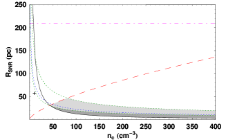
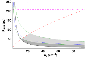
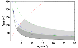
Figure 1: Constraints on the SNR radius versus cloud density for 4 different cloud radius. Top panel: $r_{c}$ = 1 pc; second panel from top: $r_{c}$ = 5 pc; third panel: $r_{c}$ = 10 pc; and bottom panel: $r_{c}$ = 20 pc. Solid (black) line: upper limit for complete cloud destruction after an encounter with an adiabatic SNR derived from Eq. 28; dashed (red) line: upper limit for the shocked cloud to reach the Jeans mass derived from Eq. 25 for an interaction with an adiabatic SNR; dotted (blue) lines: upper limits for the shock front to travel into the entire cloud before being decelerated to subsonic velocities derived from Eqs. 30 to 34 for different values of the cooling function $\Lambda(T)=10^{-25}$ (lower curve), $5\times 10^{-26}$ (middle curve), and $3\times 10^{-27}$ erg cm³ s^-1 (upper curve); dotted-dashed (pink) line: maximum radius reached by a SNR in an ISM with density n=0.05 cm^-3 and temperature T=$10^{4}$ K derived from Eq. 9. The shaded area defines the region where star formation can be induced by a SNR-cloud interaction (between the solid, dashed and dotted lines). The dark shaded zone is bounded by the $\Lambda(T)=10^{-25}$ erg cm³ s^-1 dotted (blue) curve, while the light shaded zone is bounded by the $\Lambda(T)=3\times 10^{-27}$ erg cm³ s^-1 dotted (blue) curve. The crosses in the panels indicate the initial conditions assumed for the clouds in the numerical simulations described in Section4.2 of the original manuscriptce

Few remarks are in order with regard to the Figure:

1. In the original manuscript, the dotted (blue) curves of the diagrams were built only for one value of the radiative cooling function of the shocked material, i.e. $\Lambda(T)\simeq 10^{-27}$ which is valid for a diffuse gas with a temperature $T=$ 100 K and ionization fraction $\leq$ 10^-4. Considering that the constraint established by the dotted (blue) curve in the diagrams is highly sensitive to the parameter (through Eq. 31) which in turn, can vary by two orders of magnitude depending on the value of the ionization fraction of the cloud gas, we have presently plotted in the diagrams three different dotted (blue) curves in order to cover a more realistic range of possible ionization fractions from 0.1 to 10^-4, corresponding to $\Lambda(T)=10^{-25}$ (lower dotted curve), $5\times 10^{-26}$ (middle curve), and $3\times 10^{-27}$ erg cm³ s^-1 (upper dotted curve), respectively (see Dalgarno & McCray 1972). The lower dotted (blue) curve (larger ionization fraction) bounds the dark shaded zone, while the upper one (smaller ionization fraction) bounds the light shaded zone of the diagrams. The middle dotted (blue) curve corresponds to the average value of $\Lambda$ in the range above, $5\times 10^{-26}$ erg cm³ s^-1, and could be taken as a reference.

2. In the solution presented in the original manuscript for the cloud with $r_{c}=$ 1 pc (top panel of the Figure), there was no permitted shaded zone where induction of star formation by SNR-cloud interaction would be allowed. According to the present corrections and modifications, we see that a very thin shaded ”star-formation unstable” zone appears now when the cooling function $\Lambda$ has values which are smaller than $5\times 10^{-26}$ erg cm³ s^-1, or ionization fractions $<10^{-3}$.

3. The cross labeled in the bottom panel of the Figure for a $r_{c}=$ 20 pc diffuse cloud corresponds to the initial conditions of the numerical simulations presented in Figure 6 of the original manuscript (that is, for a SNR at a distance $R_{snr}\sim$ 42 pc from the surface of the cloud). In the original manuscript, that cross lies outside the unstable shaded zone just above the upper limit for a complete shock penetration into cloud (the dotted, blue line of the diagram). With the present modifications, the cross now lies near the upper limit of the dark shaded unstable zone for values of the cooling function $\Lambda\mathrel{\hbox{\hbox to0.0pt{\hbox{\lower 4.0pt\hbox{$\sim$}}\hss}\hbox{$<$}}}10^{-25}$ erg cm³ s^-1, or ionization fractions $\mathrel{\hbox{\hbox to0.0pt{\hbox{\lower 4.0pt\hbox{$\sim$}}\hss}\hbox{$<$}}}10^{-1}$. This result remarks how sensitive the analytical diagrams are to the choice of $\Lambda$ (or the ionization fraction) for a given initial temperature cloud. According to the radiative cooling chemo-hydrodynamical simulations of Figure 6 of the original manuscript (which corresponds to the cross in the diagram), the SNR shock front really stalls within the cloud before being able to cross it completely and after all the shocked cloud material does not reach the conditions to become Jeans unstable, as predicted, but the dense cold shell that develops may fragment and later generate dense cores, as suggested in the original manuscript. This points to an ambiguity of the results due to their sensitivity to $\Lambda$ and the real ionization fraction state of the gas. We should also remark that the constraint established by the dotted (blue) curves in the diagrams is actually only an upper limit for the condition of penetration of the shock into the cloud. In order to estimate the density of the shocked material at the time $t_{st}$ when the shock stalls within the cloud (see Eq. 31 of the original manuscript or Eq. 15 of this Erratum), we have assumed pressure equilibrium between the shocked and the unshocked cloud material. A quick exam of the numerical simulations of Figure 6, however, shows that the shock front stalls before this balance is attained. This implies that the time $t_{st}$ should be smaller and therefore, the dotted (blue) curves in the diagrams should lie below the location predicted by Eq. (31).

In spite of the important alterations above in the diagrams of Figure 3, the main results and conclusions of the original manuscript of Melioli et al. (2006), particularly those regarding the young stellar system $\beta$ Pictoris, remain unchanged. Nonetheless, the present changes will be significant when compared with similar diagrams built taking into account the effects of the magnetic fields in the clouds. These will be presented in a forthcoming manuscript (Leão, de Gouveia Dal Pino and Melioli 2007, in prep.).

References

(1) Dalgarno, A., McCray, R. A., 1972, AR&AA, 10, 375
(2) Leão, M. R. M., de Gouveia Dal Pino, E. M., Melioli, C., 2007, in prep.
(3) Melioli, C., de Gouveia Dal Pino, E.M., de la Reza, R. & Raga, A., 2006, MNRAS, 373, 811
(4) Melioli, C., de Gouveia Dal Pino, E.M., & Raga, A., 2005, A&A, 443,
495