Degree and component size distributions in generalized uniform recursive tree

Abstract

We propose a generalized model for uniform recursive tree (URT) by introducing an imperfect growth process, which may generate disconnected components (clusters). The model undergoes an interesting phase transition from a singly connected network to a graph consisting of fully isolated nodes. We investigate the distributions of degree and component sizes by both theoretical predictions and numerical simulations. For the nontrivial cases, we show that the network has an exponential degree distribution while its component size distribution follows a power law, both of which are related to the imperfect growth process. We also predict the growth dynamics of the individual components. All analytical solutions are successfully contrasted with computer simulations.

Degree distribution and component (cluster) size distribution are two important properties CoRoTrVi07 of complex networks, which have become a focus of attention for the scientific community AlBa02 ; DoMe02 ; Ne03 ; BoLaMoChHw06 . It has been established that degree distribution has an important consequence on other structural characteristics of networks CoRoTrVi07 , such as average path length, clustering coefficient, betweenness centrality, and among others. Particularly, degree distribution has also profound effects on almost all aspects on dynamic processes taking place on networks, including robustness AlJeBa00 , percolation CaNeStWa00 ; CoErAvHa01 , synchronization BaPe02 , games SzFa07 , epidemic spreading PaVe01 , and so on. On the other hand, as a fundamental structural feature of networks, component (especially the giant component) size is one of the most significant measures of the network robustness AlJeBa00 ; CaNeStWa00 ; CoErAvHa01 ; in particular, component size distribution is directly related to many significant practical issues such as the distribution of the sizes of disease outbreaks for disease propagation on contact networks Gr82 ; Ne02 ; Ne07 .

A wide variety of network models has been proposed to describe real-life systems and study their structural properties AlBa02 ; DoMe02 ; Ne03 ; BoLaMoChHw06 , among which uniform recursive tree (URT) is perhaps one of the earliest and most widely studied simplest models. The URT is a growing tree constructed as follows: Start with a single node, at each increment of time, let a new node be added to the network linked to a randomly selected preexisting node. It has found applications in several areas. For example, it has been suggested as models for the spread of epidemics Mo74 , the family trees of preserved copies of ancient or medieval texts NaHe82 , chain letter and pyramid schemes Ga77 , to name but a few.

Most previous models belong to idealized models AlBa02 ; DoMe02 ; Ne03 ; BoLaMoChHw06 , although they may provide valuable insight into reality. In fact, real-world systems may be viewed as imperfect realizations of idealized theoretical models ZeKaSt07 , which have significant influences on their features and function. For instance, introducing defects (impurities) into magnetic materials may drastically change its property HuBe89 . Recently, many authors have focused on investigating the influence of deleting nodes (or edges) on the function of networks such as their integrity and communication ability AlJeBa00 ; CoErAvHa01 ; CrLaMaRa03 .

In this paper, we present a generalized model of URT by introducing an imperfect growth process which may generate disconnected components. The proposed model is governed by a tunable parameter $q$. We study both analytically and numerically the interesting characteristic aspects of the models, focusing on degree distribution, component size distribution, as well as the evolving dynamics of individual componets. We show that both distributions can be computed accurately, although calculation of component size distribution seems difficult for previously studied models. The obtained results indicate that the imperfect growth process affects fundamentally the structure of the network.

The proposed generalized model with an imperfection growth process is generated in the following way. We start from an initial state ($t=0$) of one isolated node. Then, at each increment of time, a new node is added, whose behavior of growth dynamics depends on a parameter $q$. With probability $q$, the new node keeps isolated; and with complementary probability $1-q$, the newly introduced node connects a randomly chosen old node. This growing process is repeated until the network reaches the desired size. One can easily see that at time $t$, the network consists of $t+1$ nodes and expected $(1-q)t$ edges. Thus, when $t$ is large, the average node degree at time $t$ is approximately equal to a constant value $2(1-q)$.

There are two limiting cases of the present model with URT as one of its particular case. Therefore, we call the presented model “generalized uniform recursive tree”. For $q=0$, the model coincides with the uniform recursive tree which is a singly connected network. When $q=1$, the network is reduced to a fully disconnected network. Thus, varying $q$ in the interval (0,1) allows the formation of disconnected clusters as part of the growing dynamics.

Below we will show that some interesting characteristics (i.e., degree distribution, component size distribution and evolutionary dynamics of individual components) may be investigated analytically, which depend on the parameter $q$, i.e., the imperfect growth process.

First we focus on the degree distribution. For $q=1$, all nodes have the same number of connection 0, the network exhibits a completely homogeneous degree distribution. For the case of $0\leq q<1$, we can address the degree distribution using the master-equation approach DoMeSa00 . For simplicity, we label nodes by their time of birth, so that node $s$ refers to the node introduced at time $s$, and use $p(k,s,t)$ to denote the probability that at time $t$ the node $s$ has a degree $k$. Then we may analyze the dynamics through a set of master equations DoMeSa00 ; DoMeSa01 ; ZhRoZh07 governing the evolution of the degree distribution of an individual node, which are of the following form

$$p(k,s,t+1)=\frac{1-q}{t+1}p(k - 1,s,t)+\left(1-\frac{1-q}{t+1}\right)p(k,s,t)$$ (1)

$$+ q\delta_{k,0}+(1-q)\delta_{k,1}$$

with the initial condition, $p(k,s=0,t=0)=\delta_{k,0}$. This accounts for two possibilities for a node: first, with probability $\frac{1-q}{t+1}$, it may get an extra edge from the new node, and thus increase its own degree by 1; and second, with the complimentary probability $1-\frac{1-q}{t+1}$, the node may remain in the former state with the former degree.

Based on Eq. (1), one can obtain the total degree distribution $P_{t}(k)$ specifying the probability that a randomly chosen node has degree $k$ at time $t$:

$$P_{t}(k)=\frac{1}{t+1}\sum_{s=0}^{t}p(k,s,t).$$ (2)

Summing up both sides of Eq. (1) over $s$, we get the following master equation for the degree distribution:

$$(t+2)P_{t+1}(k)-(t+1)P_{t}(k)$$

$$= (1-q)P_{t}(k-1)-(1-q)P_{t}(k)+q\delta_{k,0}+(1-q)\delta_{k,1}.$$

In the infinite $t$ limit, each $P_{t}(k)$ converges to some lime $P(k)$. Then, the corresponding stationary equation takes the form

$$(2-q)P(k)-(1-q)P(k-1)=q\delta_{k,0}+(1-q)\delta_{k,1}.$$ (4)

It has the solution of an exponential form

$$P(k)=\left\{\begin{array}[]{lc}{\displaystyle{\frac{q}{2-q},}}&\ \ k=0,\\ {\displaystyle{\frac{2}{2-q}\left(\frac{1-q}{2-q}\right)^{k},}}&\ \ k\geq 1.\\ \end{array}\right.$$ (5)

For $q=0$, Eq. (5) is exactly the same degree distribution of the uniform recursive tree DoMe02 .

Figure 1: (Color online) Semilogarithmic graph of degree distribution of the networks with order $N=200000$. Each point is an average over 10 independent simulations. The solid lines are the analytic calculation values given by Eq. (5).

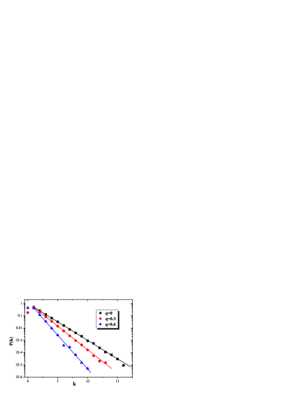
In Fig. 1, we report the simulation results of the degree distribution for several values of $q$, from which we can see that the degree distribution decays exponentially with the degree, in agreement with the analytical results.

Next, we show that the distribution of component sizes follows a power law with exponent determined by parameter $q$. For the case of $q=0$, there is only one component in the network, and the component size distribution is trivial. For $q=1$, there are $t+1$ components, every node belongs to a component of size 1 (the node itself). In the range $0<q<1$, the imperfect growth process allows the formation of multiple disconnected components. For this case, we can derive an analytical expression for the component size distribution using the rate-equation method KaReLe00 .

Initially ($t=0$), there is only one component in the network. At each subsequent step, a new cluster is created with probability $q$. Thus, after $t$ step evolution, there are expected $N(c,t)=tq+1$ components in the network, and the average value of component sizes is asymptotically equal to $\frac{1}{q}$ for large $t$. Let $N_{c}(t)$ denote the average number of components with size $c$ at time $t$. By the very construction of the generalized uniform recursive tree, when a new node enters the network, the rate equations KaReLe00 ; KaRe01 ; WaDuDaSu06 ; ZhZh07 that account for the evolution of $N_{c}(t)$ with time $t$ are

$$\frac{dN_{c}(t)}{dt}=(1-q)\frac{(c-1)N_{c-1}(t)-c\,N_{c}(t)}{{\sum_{c^{\prime}}{c^{\prime}\,N_{c^{\prime}}(t)}}}+q\,\delta_{c,1}.$$ (6)

Here the first term on the right-hand side of Eq. (6) accounts for the process in which the new node is connected to one node in a cluster with size $c-1$, leading to a gain in the number of components with size $c$. Since there are $N_{c-1}(t)$ components of size $c-1$ and the new node creates a new edge with probability $1-q$, such processes occur at a rate proportional to $(1-q)(c-1)N_{c-1}(t)$, while the factor ${\sum_{c^{\prime}}{c^{\prime}\,N_{c^{\prime}}(t)}}$ converts this rate into a normalized probability. The second (loss) term describes the new edge connecting to one of the nodes in a cluster with size $c$ turning it into a component with size $c+1$. The last term on the right-hand side of Eq. (6) accounts for the continuous introduction of a new component with size 1 (the isolated new node itself).

Let $P(c)$ be the component size distribution that is the probability of a randomly chosen cluster having size $c$. In the asymptotic limit $N_{c}(t)=N(c,t)P(c)\simeq tqP(c)$ and ${\sum_{c^{\prime}}{c^{\prime}\,N_{c^{\prime}}(t)}}=t+1$. Inserting these into Eq. (6), we have the following recursive equation

$$P(c)=\left\{\begin{array}[]{lc}{\displaystyle{\frac{c-1}{c+\frac{1}{1-q}}P(c-1),}}&\ \ c>1,\\ {\displaystyle{\frac{1}{2-q},}}&\ \ c=1,\\ \end{array}\right.$$ (7)

giving

$$P(c)=\frac{1}{2-q}\prod_{m=2}^{c}\frac{m-1}{m+\frac{1}{1-q}}=\frac{1}{2-q}\frac{\Gamma(c)\Gamma\left(2+\frac{1}{1-q}\right)}{\Gamma\left(c+1+\frac{1}{1-q}\right)}$$ (8)

for $c>1$. Thus, in the infinite $c$ limit

$$P(c)\thicksim c^{-\left(1+\frac{1}{1-q}\right)},$$ (9)

which shows that component size distribution follows a power-law form with an exponent $\gamma_{c}=1+\frac{1}{1-q}$ dependent on parameter $q$.

Figure 2: (Color online) Double-logarithmic plot of the component size distribution of the networks with 200000 nodes each. The points are the results of computer simulations, and each point is obtained by 20 independent network realizations. The solid lines correspond to the analytic solution provided by Eq. (8).

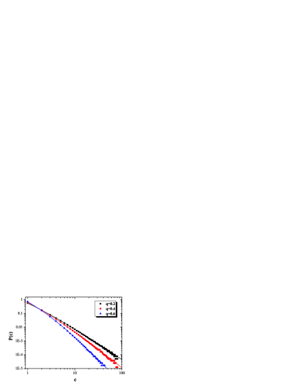
We have performed extensive numerical simulations for the full range of $q$ between 0 and 1. In Fig. 2, we plot the component size distribution $P(c)$ as a function of $q$, which agrees well with the analytic result.

In addition to component size distribution, using the continuum approach BaAlJe99 we can calculate the time dependence of component size $c_{i}$ of a given component $i$, $i=1,2,\cdots,N(c,t)$. The size will increase by one every time a new node is added to the system and linked to one of the nodes belonging to this component. Assuming that $c_{i}$ is a continuous real variable, according to the generating algorithm of the model, the rate at which $c_{i}$ changes is clearly proportional to $c_{i}$ itself. Consequently $c_{i}$ satisfies the dynamical equation BaAlJe99 ; ZhRoCo06

$$\frac{\partial c_{i}(t)}{\partial t}=(1-q)\frac{c_{i}(t)}{t}.$$ (10)

The solution of this equation, with the initial condition that component $i$ was born at time $t_{i}$ with size $c_{i}(t_{i})=1$, is

$$c_{i}(t)=\left(\frac{t}{t_{i}}\right)^{1-q}.$$ (11)

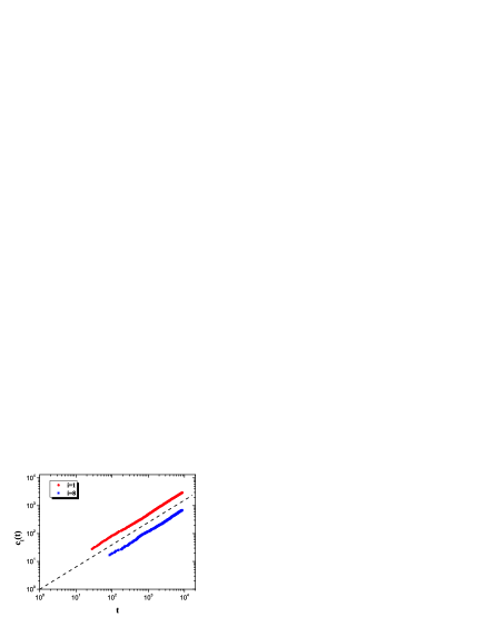
Equation (11) shows that the size of all components evolves the same way, following a power law, the only difference being the intercept of this power law, see Fig. 3.

Figure 3: (Color online) Double-logarithmic graph showing the time-evolution for the sizes of two components. Here $q=0.2$, and the dashed line has slope 0.8, as predicted by Eq. (11).

To conclude, by introducing an imperfect network growth process we have proposed an extended model for uniform recursive tree. The presented model interpolates between a network with fully disconnected clusters and the uniform recursive tree with only one single component, which allow us to explore the crossover between the two limiting cases. We have provided both analytically and numerically the solutions for degree and component size distributions of our model. We found that in the case of $0<q<1$ the model exhibits an exponential degree distribution and a power-law component size distribution. We also presented that the size of all components evolves as a power-law function of time $t$.

Our model has a remarkable character that some nodes may become disconnected from the rest of the network. This property has been less reported in earlier studied models and thus has not yet been paid enough attention to. Actually, our model may be further extended to include initial attractiveness DoMeSa00 and preferential attachment BaAl99 . That is, all nodes are born with some initial attractiveness $A>0$. In the growth progress, the probability that an old node will receive an link from the new old is proportional to the sum of the initial attractiveness and its degree. In this more general case, the degree distribution is power law with exponent dependent on $A$, while the component size distribution is the same as that of the present model addressed here and is independent of parameter $A$. Finally, we believe our model could stimulate and find some obvious implications for some related researches such as disease propagation in future.

This research was supported by the National Basic Research Program of China under grant No. 2007CB310806, the National Natural Science Foundation of China under Grant Nos. 60496327, 60573183, 90612007, 60773123, and 60704044, the Postdoctoral Science Foundation of China under Grant No. 20060400162, the Program for New Century Excellent Talents in University of China (NCET-06-0376), and the Huawei Foundation of Science and Technology (YJCB2007031IN).

References

- (1) L. da. F. Costa, F.A. Rodrigues, G. Travieso, and P.R.V. Boas, Adv. Phys. 56, 167 (2007).
- (2) R. Albert and A.-L. Barabási, Rev. Mod. Phys. 74, 47 (2002).
- (3) S.N. Dorogvtsev and J.F.F. Mendes, Adv. Phys. 51, 1079 (2002).
- (4) M.E.J. Newman, SIAM Rev. 45, 167 (2003).
- (5) S. Boccaletti, V. Latora, Y. Moreno, M. Chavez and D.-U. Hwanga, Phys. Rep. 424, 175 (2006).
- (6) R. Albert, H. Jeong, A.-L. Barabási, Nature (London) 406, 378 (2000).
- (7) D. S. Callaway, M. E. J. Newman, S. H. Strogatz, and D. J. Watts, Phys. Rev. Lett. 85, 5468 (2000).
- (8) R. Cohen, K. Erez, D. ben-Avraham, S. Havlin Phys. Rev. Lett. 86, 3682 (2001).
- (9) M. Barahona and L. M. Pecora, Phys. Rev. Lett. 89, 054101 (2002).
- (10) G. Szabó and G. Fáth, Phy. Rep. 446, 97 (2007).
- (11) R. Pastor-Satorras and A. Vespignani, Phys. Rev. Lett. 86, 3200 (2001).
- (12) P. Grassberger, Math. Biosci. 63, 157 (1982).
- (13) M. E. J. Newman, Phys. Rev. E 66, 016128 (2002).
- (14) M. E. J. Newman, Phys. Rev. E 76, 045101(R) (2007).
- (15) J. W. Moon, London Math. Soc. Lecture Note 13, 125 (1974).
- (16) D. Najock and C. Heyde, J. Appl. Prob. 19, 675 (1982).
- (17) J. Gastwirth, Amer. Statist. 31, 79 (1977).
- (18) A. Zen, A. Kabakçıoğlu, and A. L. Stella, Phys. Rev. E 76, 026110 (2007).
- (19) K. Hui and A. N. Berker, Phys. Rev. Lett. 62, 2507 (1989).
- (20) P. Crucitti, V. Latora, M. Marchiori, and A. Rapisarda, Physica A 320, 622 (2003).
- (21) S.N. Dorogovtsev, J.F.F. Mendes, and A.N. Samukhin, Phys. Rev. Lett. 85, 4633 (2000).
- (22) S.N. Dorogovtsev, J.F.F. Mendes, and A.N. Samukhin, Phys. Rev. E 63, 062101 (2001).
- (23) Z. Z. Zhang, S. G. Zhou, Z. Shen, and J. H. Guan, Physica A 385, 765 (2007).
- (24) P.L. Krapivsky, S. Redner, and F. Leyvraz, Phys. Rev. Lett. 85, 4629 (2000).
- (25) P. L. Krapivsky and S. Redner, Phys. Rev. E 63, 066123 (2001).
- (26) L. Wang L, F. Du, H. P. Dai, and Y. X. Sun, Eur. Phys. J. B 53, 361 (2006).
- (27) Z.Z. Zhang and S. G. Zhou, Physica A 380, 621 (2007).
- (28) A.-L. Barabási, R. Albert, and H. Jeong, Physica A 272, 173 (1999).
- (29) Z.Z. Zhang, L.L. Rong, and F. Comellas, Physica A 364, 610 (2006).
- (30) A.-L. Barabási and R. Albert, Science 286, 509 (1999).