Moduli flow and non-supersymmetric AdS attractors

Abstract:

We investigate the attractor mechanism in gauged supergravity in the presence of higher derivatives terms. In particular, we discuss the attractor behaviour of static black hole horizons in anti-de Sitter spacetime by using the effective potential approach as well as Sen’s entropy function formalism. We use the holographic techniques to interpret the moduli flow as an RG flow towards the IR attractor horizon. We find that the holographic c-function obeys the expected properties and point out some subtleties in understanding attractors in AdS.

1 Introduction

Black holes are testing grounds for string theory as a theory of quantum gravity. The Bekenstein-Hawking entropy is inherently quantum gravitational, involving both the Newtons’s constant $G_{N}$ and Planck’s constant $\hbar$. Therefore, any consistent theory of quantum gravity should address the origin of black hole entropy.

The ‘holographic’ principle, [1, 2], was formulated as an attempt at understanding the physics of quantum black holes and at reconciling gravitational collapse and unitarity of quantum mechanics at the Planck scale. Thus, it is very tempting to consider the holographic principle as a simple organizing principle for quantum gravity. String theory provides a concrete realization of the holographic principle for spacetimes with negative cosmological constant, namely the anti-de Sitter (AdS)/CFT correspondence [3]. That is a non-perturbative background independent definition of quantum gravity in asymptotically AdS spaces. On the other hand, string theory provides a microscopic description for the entropy of certain types of black holes through the counting of D-branes bound states [4, 5].

AdS black holes in gauged supergravity theories have found widespread application in the study of the AdS/CFT correspondence (see, e.g., [6] and references therein). BPS objects are important within AdS/CFT duality, regardless of their precise nature, since their properties remain the same in both the strong and weak coupling regimes of the duality. However, it is also useful to investigate properties of non-BPS objects in this context — this is the topic of the present investigation.

The attractor mechanism plays a key role in understanding the entropy of asymptotically flat non-supersymmetric extremal black holes in string theory [7, 8, 9] and so it is of great interest to study the attractor behaviour of extremal black hole horizons in AdS.

The attractor mechanism was discovered in the context of $N=2$ supergravity [10], then extended to other supergravity theories [11]. It is now well understood that supersymmetry does not really play a fundamental role in the attractor phenomenon. The attractor mechanism works as a consequence of the symmetry of the near horizon extremal geometry that is given by $AdS_{2}\times S^{p}$ [12] for static spherically symmetric black holes — in fact, the ‘long throat’ of $AdS_{2}$ (see [13])is at the basis of the attractor mechanism [12, 14, 15].

One can understand why the near horizon geometry is more important than supersymmetry by analogy with the flux compactifications: $AdS_{2}\times S^{2}$ can be interpreted as a flux compactification on $S^{2}$. This way, the flux generates an effective potential for the moduli such that, at the horizon, the potential has a stable minimum and the moduli are stabilized. Unlike the non-extremal case where the near horizon geometry (and the entropy) depends on the values of the moduli at infinity, in the extremal case the near horizon geometry is universal and is determined by only the charge parameters. Consequently, the entropy is also independent of the asymptotic values of the moduli.

In this paper we study the attractor mechanism in AdS spacetime in the presence of higher derivatives terms. We focus on static $5$-dimensional charged black hole solutions in gravity theories with $U(1)$ gauge fields and neutral massless scalars. The extremal black holes in AdS have also an $AdS_{2}\times S^{3}$ geometry in the near horizon limit, hence the analogy would indicate that the attractor mechanism should also work for this kind of black holes.

Following [17](for related work, see [18]), we use perturbative methods and numerical analysis to show that the horizons of extremal black holes in AdS (with Gauss-Bonet term) are attractors — this analysis supports the existence of the attractor mechanism for black holes in AdS space with higher derivatives.

We will provide a physical interpretation for the attractor mechanism within the AdS/CFT duality. This requires the embedding in string theory that is explicitly constructed. Once we embed the solutions in 10 dimensional IIB supergravity (and so in string theory), we can use the AdS/CFT correspondence to interpret the moduli flow as a holographic renormalization group (RG) flow.

To complete our analysis of the attractor mechanism within AdS/CFT duality, we will construct a c-function that obeys the expected results, namely it decreases monotonically as the radial coordinate is decreasing. Therefore, within the AdS/CFT correpondence, there is a concrete connection between the attractor mechanism (gravity side) and the ‘dual’ universality property of the QFT. The idea (reffered to as ‘universality’ of QFT) that the IR end-point of a QFT RG flow does not depend upon UV details becomes in the holography context the statement that the bulk solution for small values of $r$ does not depend upon the details of the matter at large values of $r$. Indeed, within the attractor mechanism, the black hole horizon (IR region) does not have any memory of the initial conditions (the UV values of the moduli) at the boundary. The black hole entropy depends just on the charges and not on the asymptotic values of the moduli. However, we can interpret it as a ‘no-hair’ theorem for the extremal black holes in AdS that is equivalent with the ‘universality’ of the field theory on the brane [19].

The paper is organized as follows: In section 2 we discuss the attractor mechanism in two derivatives gauged supergravity. Our discussion is general in that it is based on analysis of the equations of motion, not just the near horizon geometry and its symmetries. We show the equivalence of the effective potential approach [17] and the entropy function formalism [12] in the near horizon limit of the extremal black holes in AdS. In section 3 we examine the attractor mechanism in AdS gravity with higher derivatives. We generalize the effective potential in the Gauss-Bonnet gravity and find that even in this case the extremal black hole horizon is a stable minimum of the effective potential. Consequently, the moduli are stabilized and the entropy does not depend on couplings. In section 4 we present a holographic interpretation for the attractor mechanism by identifying the moduli flow with the RG flow and also find the c-function. Finally, we end with a discussion of our results in section 5.

2 Attractors in two derivatives gauged supergravity

In this section we generalize the results of [17] by including a potential for the scalar fields in the action. We discuss the attractor mechanism using both the effective potential method [17] and the entropy function framework [12]. The first method is based on investigating the equations of motion of the moduli and finding the conditions satisfied by the effective potential such that the attractor phenomenon occurs. The entropy function approach is based on the near horizon geometry and its enhanced symmetries.

2.1 Generalities

While details of the various supergravity theories depend crucially on the dimension, general features of the bosonic sector can be treated in a dimension independent manner. However, from now on, we will focus on a 5-dimensional theory of gravity coupled to a set of massless scalars and vector fields, whose general bosonic action has the form

$$I[G_{\mu\nu},\phi^{i},A_{\mu}^{I}]\! = \!\frac{1}{\kappa^{2}}\int_{M}d^{5}x\sqrt{-G}[R-g_{ij}(\phi)\partial_{\mu}\phi^{i}\partial^{\mu}\phi^{j}$$ (1)

$$-f_{AB}(\phi)F^{A}_{\mu\nu}F^{B\,\mu\nu}+V(\phi)]$$

where $F^{A}_{\mu\nu}$ with $A=(0,\cdots N)$ are the gauge fields, $\phi\equiv(\phi^{i})$ with $i=(1,\cdots,n$) are the scalar fields, $V(\phi^{i})$ is the scalar fields potential, and $\kappa^{2}=16\pi G_{N}$. The moduli determine the gauge coupling constants and $g_{ij}(\phi)$ is the metric in the moduli space. We use Gaussian units so that factors of $4\pi$ in the gauge fields can be avoided and the Newton’s constant $G_{N}$ is set to $1/16\pi$. The above action is of the type of the $gauged$ supergravity theories.

The equations of motion for the metric, moduli, and the gauge fields are given by

$$R_{\mu\nu}-g_{ij}\partial_{\mu}\phi^{i}\partial_{\nu}\phi^{j}=f_{AB}\left(2F^{A}_{\phantom{A}\mu\lambda}F^{B\phantom{\nu}\lambda}_{\phantom{B}\nu}-{\textstyle\frac{1}{3}}G_{\mu\nu}F^{A}_{\phantom{a}\alpha\lambda}F^{B\alpha\lambda}\right)-\frac{1}{3}G_{\mu\nu}V(\phi)\,$$ (2)

$$\frac{1}{\sqrt{-G}}\partial_{\mu}(\sqrt{-G}g_{ij}\partial^{\mu}\phi^{j})=\frac{1}{2}\left(\frac{\partial f_{AB}}{\partial\phi^{i}}F^{A}_{\phantom{A}\mu\nu}F^{B\,\mu\nu}+\frac{\partial g_{mn}}{\partial\phi^{i}}\partial_{\mu}\phi^{m}\partial^{\mu}\phi^{n}-\frac{\partial V(\phi)}{\partial\phi^{i}}\right)\,$$ (3)

$$\partial_{\mu}\left[\sqrt{-G}\left(f_{AB}F^{B\,\mu\nu}\right)\right]=0\,$$ (4)

where we have varied the moduli and the gauge fields independently. The Bianchi identities for the gauge fields are $F_{\phantom{A}\,[\mu\nu;\lambda]}^{A}=0$.

We focus on $5$-dimensional spherically symmetric spacetime metrics and we consider the following ansatz:

$$ds^{2} = -a(r)^{2}dt^{2}+a(r)^{-2}dr^{2}+b(r)^{2}d\Omega_{3}^{2}$$ (5)

We consider a definite form of the 3-sphere

$$d\Omega^{2}_{3} = d\theta^{2}+\sin^{2}\theta\,d\phi^{2}+\cos^{2}\theta\,d\psi^{2}\,$$ (6)

with coordinate ranges $\theta\in[0,\frac{\pi}{2}]$ and $\phi,\psi\in[0,2\pi]$.

The Bianchi identity and equation of motion for the gauge fields can be solved by a field strength of the form [17]

$$F^{A}=\frac{1}{b^{3}}f^{AB}Q_{B}\;dt\wedge dr$$ (7)

where $Q_{A}$ are constants which determine electric charges carried by the gauge field $F^{A}$ and $f^{AB}$ is the inverse of $f_{AB}$.

With this ansatz, the gravitational equations of motion become

$$R_{rr} = -\frac{1}{a^{2}b}\left(b(a^{\prime 2}+aa^{\prime\prime})+3a(a^{\prime}b^{\prime}+ab^{\prime\prime})\right)$$

$$= \phi^{\prime 2}-\frac{4}{3a^{2}b^{6}}\,f^{AB}Q_{A}Q_{B}-\frac{1}{3a^{2}}\,V(\phi)\,$$

$$R_{tt} = a^{2}(a^{\prime 2}+\frac{3aa^{\prime}b^{\prime}}{b}+aa^{\prime\prime})$$

$$= \frac{4a^{2}}{3b^{6}}f^{AB}Q_{A}Q_{B}+\frac{1}{3}a^{2}V(\phi)\,$$

$$R_{\theta\theta} = 2-2aba^{\prime}b^{\prime}-a^{2}(2b^{\prime 2}+bb^{\prime\prime})$$

$$= \frac{2}{3b^{4}}f^{AB}Q_{A}Q_{B}-\frac{1}{3}b^{2}V(\phi)$$

Here we use the notation $\phi^{\prime 2}=g_{ij}\partial_{r}\phi^{i}\partial^{r}\phi^{j}$. Note that $R_{\phi\phi}=\sin^{2}\theta R_{\theta\theta},~{}R_{\psi\psi}=\cos^{2}\theta R_{\theta\theta},$ and that off-diagonal components of the Ricci and stress tensors vanish. It is also important to notice that the field equations are not all independent.

It is easier to use combinations of the equations above

$$R_{tt}+2\frac{G_{tt}}{G_{\theta\theta}}R_{\theta\theta}\,,\hskip 14.22636ptR_{rr}-\frac{G_{rr}}{G_{tt}}R_{tt}\,,\hskip 14.22636pt-\frac{G_{\theta\theta}}{G_{tt}}R_{tt}+\frac{G_{\theta\theta}}{G_{rr}}R_{rr}-3R_{\theta\theta}$$ (11)

and from now on we will work with the following equivalent system of differential equations:

$$0 = 4(-1+a^{2}b^{\prime 2})+(a^{\prime 2}+aa^{\prime\prime})b^{2}+ab(7a^{\prime}b^{\prime}+2ab^{\prime\prime})-b^{2}V(\phi_{i})$$ (12)

$$0 = \phi^{\prime 2}+3\frac{b^{\prime\prime}}{b}$$ (13)

$$0 = -1+aba^{\prime}b^{\prime}+a^{2}b^{\prime 2}-\frac{1}{6}a^{2}b^{2}\phi^{\prime 2}-\frac{1}{6}\;b^{2}V(\phi_{i})+\frac{V_{eff}}{3b^{4}}$$ (14)

We should also consider the equations of motion for the scalars which can be written as

$$\partial_{r}(a^{2}b^{3}\partial_{r}\phi_{i})=\frac{1}{b^{3}}(\partial_{i}V_{eff}-\frac{1}{2}b^{6}\partial_{i}V)$$ (15)

where $V_{eff}=f^{AB}Q_{A}Q_{B}$ and $f^{AB}$ is the inverse of $f_{AB}$. When the scalar potential $V(\phi)$ is constant, $V_{eff}(\phi^{i})$ plays the role of an ‘effective potential’ that is generated by non-trivial form fields. The effective potential, first discussed in [20], plays an important role in describing the attractor mechanism [17, 21].

A vanishing Hamiltonian is a characteristic feature of any theory which is invariant under arbitrary coordinate transformations — for our system, the equation (14) does not contain any second derivatives and is the Hamiltonian constraint.

As a final comment, we observe that the equations of motion can also be obtained from the following one-dimensional action

$$S=\frac{1}{\kappa^{2}}\int dr\left(6b+6ab^{2}a^{\prime}b^{\prime}+6a^{2}bb^{\prime 2}+b^{3}V(\phi)-a^{2}b^{3}(\phi_{i}^{\prime})^{2}-\frac{2}{b^{3}}V_{eff}(\phi_{i})\right)$$ (16)

2.2 Entropy function

We apply the entropy function formalism to static black holes in AdS space. It was shown by Sen that the attractor mechanism is related to the extremality (attempts to apply the entropy function to non-extremal black holes can be found in [23]) rather than to the supersymmetry property of a given solution. Indeed, the $AdS_{2}$ factor of the near-horizon geometry is at the basis of the attractor mechanism. As has been discussed in [24, 15], the moduli do not preserve any memory of the initial conditions at infinity due to the presence of the infinite throat of $AdS_{2}$. This is in analogy with the properties of the behaviour of dynamical flows in dissipative systems, where, on approaching the attractors, the orbits practically lose all the memory of their initial conditions.

Therefore, an important hint for the existence of the attractor meachanism is the existence of an $AdS_{2}$ as part of the near horizon geometry of an extremal black hole. The extremal charged black hole solution of the equations of motion with constant scalar fields is the extremal Reissner-Nordstrom-anti-de Sitter (RNadS) black hole given by [25]

$$a^{2}(r)=1+\frac{r^{2}}{l^{2}}-\frac{m}{r^{2}}+\frac{q^{2}}{r^{4}}=\frac{1}{l^{2}r^{4}}(r-r_{H})^{2}(r+r_{H})^{2}(r^{2}+2r_{H}^{2}+l^{2})$$ (17)

Here $r=r_{H}$ is the degenerate horizon and can be calculated using the following expressions of mass and charge parameter:

$$m=2r_{H}^{2}\left(1+\frac{3}{2}\frac{r_{H}^{2}}{l^{2}}\right),\hskip 17.07182ptq^{2}=r_{H}^{4}\left(1+2\frac{r_{H}^{2}}{l^{2}}\right)$$ (18)

The mass parameter $m$ and the charge parameter $q$ are related to the asymptotic ADM charges $M$ and $Q$ by:

$$M=\frac{3\pi}{8G_{N}}m\,,\hskip 28.45274ptQ=\sqrt{3}q$$ (19)

and the electric field is given by

$$F=\frac{1}{2}F_{\mu\nu}dx^{\mu}\wedge dx^{\nu}=\frac{Q}{r^{3}}dr\wedge dt\,$$ (20)

In the near horizon limit, $\rho=r-r_{H}\rightarrow 0$, we obtain

$$a(\rho)=\frac{4}{l^{2}r_{H}^{2}}(3r_{H}^{2}+l^{2})\,\rho^{2}=\frac{1}{v_{1}}\,\rho^{2}$$ (21)

where $v_{1}$ is a constant that can be interpreted as the radius of $AdS_{2}$ — the $AdS_{2}\times S^{3}$ geometry appears explicitly by making the change of coordinates $t=v_{1}\tau$.

It is important to notice that the extremal solution is non-supersymmetric. The supersymmetric bound is $M=2Q$ and in this limit one finds a naked curvature singularity at $r=0$. However, by adding $\alpha^{\prime}$-corrections this singularity may be dressed by a horizon with finite area.

Let us now briefly review the entropy function formalism. In [12] (see also [26]), it was observed that the entropy of a spherically symmetric extremal black hole is the Legendre transform of the Lagrangian density. The derivation of this result does not require the theory and/or the solution to be supersymmetric. The only requirements are gauge and general coordinate invariance of the action.

The entropy function is defined as

$$F(\overrightarrow{u},\overrightarrow{v},\overrightarrow{e},\overrightarrow{p})=2\pi(e_{i}q_{i}-f(\overrightarrow{u},\overrightarrow{v},\overrightarrow{e},\overrightarrow{p})=2\pi(e_{i}q_{i}-\int d\theta d\phi d\psi\sqrt{-G}{\cal L})$$ (22)

where $q_{i}=\partial f/\partial e_{i}$ are the electric charges, $u_{s}$ are the values of the moduli at the horizon, ${p_{i}}$ and ${e_{i}}$ are the near horizon radial magnetic and electric fields and $v_{1}$, $v_{2}$ are the sizes of $AdS_{2}$ and $S^{2}$ respectively. Thus, $F/2\pi$ is the Legendre transform of the function $f$ with respect to the variables $e_{i}$.

For an extremal black hole of electric charge $\overrightarrow{Q}$ and magnetic charge $\overrightarrow{P}$, Sen has shown that the equations determining $\overrightarrow{u},\overrightarrow{v}$, and $\overrightarrow{e}$ are given by:

$$\frac{\partial F}{\partial u_{s}}=0\,,\qquad\frac{\partial F}{\partial v_{i}}=0\,,\qquad\frac{\partial F}{\partial e_{i}}=0\,$$ (23)

Then, the black hole entropy is given by $S=F(\overrightarrow{u},\overrightarrow{v},\overrightarrow{e},\overrightarrow{p})$ at the extremum (23). The entropy function, $F(\overrightarrow{u},\overrightarrow{v},\overrightarrow{e},\overrightarrow{p})$, determines the sizes $v_{1}$, $v_{2}$ of $AdS_{2}$ and $S^{3}$ and also the near horizon values of moduli ${u_{s}}$ and gauge field strengths ${e_{i}}$. If $F$ has no flat directions, then the extremization of $F$ determines $\overrightarrow{u}$, $\overrightarrow{v}$, $\overrightarrow{e}$ in terms of $\overrightarrow{Q}$ and $\overrightarrow{P}$. Therefore, $S=F$ is independent of the asymptotic values of the scalar fields. These results lead to a generalised attractor phenomenon for both supersymmetric and non-supersymmetic extremal black hole solutions.

Now we are ready to apply this method to our action (1). The general metric of $AdS_{2}\times S^{3}$ can be written as

$$ds^{2}=v_{1}(-\rho^{2}d\tau^{2}+\frac{1}{\rho^{2}}d\rho^{2})+v_{2}d\Omega_{3}^{2}\,$$ (24)

The field strength ansatz (7) in our case is given by

$$F^{A}=e^{A}d\tau\wedge d\rho.$$ (25)

The entropy function $F(u^{i},v_{1},v_{2},e^{A},Q_{A})$ and $f(u^{i},v_{1},v_{2},e^{A})$ are given by

$$F(u^{i},v_{1},v_{2},e^{A},Q_{A})=2\pi[Q_{A}e^{A}-f(u^{i},v_{1},v_{2},e^{A})]\,,$$ (26)

$$f(u^{i},v_{1},v_{2},e^{A})=2\pi^{2}\left[-2v_{2}^{3/2}+6v_{1}\sqrt{v_{2}}+2\frac{v_{2}^{3/2}}{v_{1}}f_{AB}e^{A}e^{B}+v_{1}v_{2}^{3/2}V(\phi)\,\right]\,$$

Then the attractor equations are obtained as :

$$\frac{\partial F}{\partial v_{1}} = 0\,\,\,\Rightarrow\,\,\,6v_{1}^{2}-2v_{2}f_{AB}e^{A}e^{B}+v_{1}^{2}v_{2}V(\phi)=0\,$$ (27)

$$\frac{\partial F}{\partial v_{2}} = 0\,\,\,\Rightarrow\,\,\,-v_{1}v_{2}+v_{1}^{2}+v_{2}f_{AB}e^{A}e^{B}+\frac{v_{1}^{2}v_{2}}{2}V(\phi)=0\,$$ (28)

$$\frac{\partial F}{\partial u^{i}} = 0\,\,\,\Rightarrow\,\,\,\,2\frac{\partial f_{AB}}{\partial u^{i}}e^{A}e^{B}=-v^{2}_{1}\frac{\partial V}{\partial u^{i}}$$ (29)

$$\frac{\partial F}{\partial e^{A}} = 0\,\,\,\Rightarrow\,\,\,Q_{A}=8\pi^{2}\,\frac{v_{2}^{3/2}}{v_{1}}f_{AB}e^{B}\,$$ (30)

By combining the first two equations we obtain $4/v_{2}-1/v_{1}+V(\phi)=0$ and so the radii of $AdS_{2}$ and $S^{3}$ are related by the potential of the scalars. By replacing (27) and (30) in (26) we obtain the value of the entropy function at the extremum, $F=8\pi^{3}v_{2}^{3/2}$, that is the entropy of the black hole (our convention was $G_{N}=1/16\pi$).

The third equation is very important: in AdS spacetime, $V(\phi)=constant$, this equation is equivalent with finding the critical points of the effective potential at horizon. One can easily eliminate the field strengths in the favour of charges by using the last equation to obtain $(\partial f^{AB}/\partial u^{i})\,Q_{A}Q_{B}=0$ — we will show in the next subsection that this is one of the conditions for the existence of attractor mechanism. If this equations has solutions, then the moduli values at the horizon are fixed in term of the charges. It is also important to notice that the existence of a near-horizon geometry when the moduli are not constants does not imply the existence of the whole solution in the bulk (from the horizon to the boundary) — this is the disadvantage of the entropy function formalism. However, in the next subsection we will investigate the equations of motion in the bulk and describe the horizon as an IR critical point of the effective potential.

2.3 Effective potential and non-supersymmetric attractor

In this section we consider a constant potential for scalars, $V(\phi)=12/l^{2}$. For the attractor phenomenon to occur, it is sufficient if the following two conditions are satisfied [17]. First, for fixed charges, as a function of the moduli, $V_{eff}$ must have a critical point. Denoting the critical values for the scalars as $\phi^{i}=\phi^{i}_{0}$ we have,

$$\partial_{i}V_{eff}(\phi^{i}_{0})=0$$ (31)

Second, there should be no unstable directions about this minimum, so the matrix of second derivatives of the potential at the critical point,

$$M_{ij}=\frac{1}{2}\partial_{i}\partial_{j}V_{eff}(\phi^{k}_{0})$$ (32)

should have no negative eigenvalues. Schematically we can write,

$$M_{ij}>0$$ (33)

We will refer to $M_{ij}$ as the mass matrix and its eigenvalues as masses (more correctly $mass^{2}$ terms) for the fields, $\phi^{i}$.

It is important to note that in deriving the conditions for the attractor phenomenon, one does not have to use supersymmetry at all. The extremality condition puts a strong constraint on the charges so that the asymptotic values of the moduli do not appear in the entropy formula.

2.3.1 Zeroth order analysis

Let us start by setting the asymptotic values of the scalars equal to their critical values (independent of $r$), $\phi^{i}=\phi^{i}_{0}$. The equations of motion (13, 12) can be easily solved. First we solve (13) and get $b(r)=r$, and then replace this expression in (12) — we obtain:

$$\frac{1}{2}r^{2}(a^{2})^{\prime\prime}+\frac{7}{2}r(a^{2})^{\prime}+4a^{2}=4+\frac{12}{l^{2}}r^{2}.$$ (34)

The most general solution of this equation is given by $a^{2}(r)=1+C_{1}/r^{2}+C_{2}/r^{4}+r^{2}/l^{2}$, where $C_{1}$ and $C_{2}$ are integration constants. We are interested in the extremal solutions and so the integration constants can be calculated from the ‘double horizon’ condition:

$$C_{2}=-(\frac{3r_{H}^{4}}{l^{2}}+2r_{H}^{6}),\;\;\;\;\;C_{1}=r_{H}^{4}+\frac{2r_{H}^{6}}{l^{2}},$$ (35)

where $r_{H}$ is the horizon radius. Therefore, we can write the solution as

$$a_{0}(r)=(1-\frac{r_{H}^{2}}{r^{2}})\sqrt{1+\frac{r^{2}+2r_{H}^{2}}{l^{2}}},\;\;\;\ b_{0}(r)=r,$$ (36)

that describes the extremal RNadS found in the previous subsection.

The Hamiltonian constraint evaluated at the boundary provides a constraint on charges. However, we are interested in solving the Hamiltonian constraint at the horizon and to obtain a relation between the entropy and the effective potential. It is important to notice that the temperature is proportional to $aa^{\prime}$ and so just in the extremal limit this product is vanishing. With this observation the Hamiltonian constraint simplifies drastically at the horizon. Thus, the horizon radius, $r_{H}$, can be computed from the following equation:

$$-3r_{H}^{4}-\frac{6}{l^{2}}r_{H}^{6}+V_{eff}(\phi^{i}_{0})=0.$$ (37)

We obtain ($f_{AB}=1$)

$$Q^{2}=3r_{H}^{4}\,\left(1+2\frac{r_{H}^{2}}{l^{2}}\right),$$ (38)

that is the $ADM$ electric charge (19) of the extremal RNadS black hole.

2.3.2 First order analysis

For the extremal RNadS black hole solution carrying the charges specified by the parameter $Q_{A}$ and the moduli taking the critical values $\phi^{i}_{0}$ at infinity, a double zero horizon continues to exist for small deviations from these attractor values for the moduli at infinity. The moduli take the critical values at the horizon and entropy remains independent of the values of the moduli at infinity [17]. The horizon radius is given by the eq. (37) and the entropy is

$$S_{BH}=\frac{A}{4G_{N}}=\frac{\pi^{2}}{2G_{N}}r_{H}^{3}=8\pi^{3}r_{H}^{3}$$ (39)

We start with first order perturbation theory

$$\delta\phi_{i}=\phi_{i}-\phi_{i0}=\epsilon\phi_{i1}$$ (40)

where $\epsilon$ is a small parameter we use to organize the perturbation theory. The first correction to the scalars $\phi_{i}$ satisfies the equation

$$\partial_{r}(a_{0}^{2}b_{0}^{3}\partial_{r}\phi_{i1})=\frac{\beta_{i}^{2}}{b_{0}^{3}}\phi_{i1}$$ (41)

where $\beta_{i}^{2}$ is the eigenvalue for the matrix $2M_{ij}$. We are interested in a ‘smooth’ solution that does not blow up at horizon $r=r_{H}$. It is difficult to find a general solution — however we will study our equations in the near horizon limit (the solution in the asymptotic region is presented in Section 4) and keep in mind that there is a smooth interpolation between the horizon and the boundary. In the near horizon limit, we obtain

$$\phi_{i1}=c_{1i}(1-\frac{r_{H}}{r})^{\gamma_{i}}$$ (42)

where $\gamma_{i}$ are positive roots of following equations

$$\gamma_{i}(\gamma_{i}+1)=\frac{\beta_{i}^{2}}{4r_{H}^{4}}(1+\frac{3r_{H}^{2}}{l^{2}})^{-1}$$ (43)

Asymptotically (as $r\rightarrow\infty$) $\phi_{i1}$ takes a constant value, $c_{1i}$ — however $\phi_{i1}$ is vanishing at the horizon and the value of the scalar is fixed at $\phi_{i0}$ regardless of its value at infinity. We observe from the equation (43) that if the eigenvalues of the mass matrix are positive, then the solution is regular at the horizon and so the existence of a regular horizon is related to the existence of the attractor mechanism. In the light of previous discussions, this is easy to understand if we recall that the near horizon geometry of an extremal black hole is $AdS_{2}\times S^{3}$.

2.3.3 Second order analysis and back reaction

The first perturbation in scalars sources a second order correction in the metric. We write

$$a = a_{0}+a_{2}\epsilon^{2}$$ (44)

$$b = b_{0}+b_{2}\epsilon^{2}$$ (45)

and by solving the equations (12) and (13) we obtain

$$a(r) = (1-\frac{r_{H}^{2}}{r^{2}})\sqrt{1+\frac{r^{2}+2r_{H}^{2}}{l^{2}}}\left(1+a_{i2}(1-\frac{r_{H}}{r})^{2\gamma_{i}}\right)$$ (46)

$$b(r) = r\left(1+b_{i2}(1-\frac{r_{H}}{r})^{2\gamma_{i}}\right)$$ (48)

where

$$a_{i2} = -b_{i2}\left(\frac{1}{(\gamma_{i}+1)(2\gamma_{i}+1)(1+\frac{3r_{H}^{2}}{l^{2}})}+\frac{\gamma_{i}(4\gamma_{i}+5)}{(\gamma_{i}+1)(2\gamma_{i}+1)}\right)$$ (49)

$$b_{i2} = -\frac{\gamma_{i}c_{1i}^{2}}{6(2\gamma_{i}-1)}$$ (50)

We see that in second order we need to choose again positive $\gamma_{i}$ in order to get a regular horizon. That means the small fluctuations about the extremal point must all be positive and so the horizon is an attractor. Thus, in the near horizon limit we obtain again the near horizon geometry of the extremal RNadS black hole that is fixed only by the charges.

2.4 Higher order result

Going to higher orders in perturbation theory is in principle straightforward. We solve the system of equations (12)-(14) order by order in the $\epsilon$-expansion. To first order, we find that one variable, say $c_{1i}$ , can not be fixed by the equations. Thus we find $a_{i2}$ and $b_{i2}$ as functions of $c_{1i}$. One can check that at any order $n>2$, one can substitute the resulting values of ($a_{mi},b_{mi},\phi_{mi}$ ), for all $m\leq n$ from the previous orders. Then (12)-(14) of the order $m$, consistently give,

$$a_{mi}=a_{mi}(c_{1i}),\;\;\;\;b_{mi}=b_{mi}(c_{1i}),\;\;\;\;\phi_{mi}=\phi_{mi}(c_{1i}),$$ (51)

as polynomials of order n in terms of $c_{1i}$. It is worth noting that $c_{1i}$ remains a free parameter to all orders in the $\epsilon$- expansion. Owing to the result above, we observe that $(a_{\infty i},b_{\infty i},\phi_{\infty i})$ are varying and will take different values, given different choices for $c_{1i}$. The arbitrary value of $\phi_{i}$ at infinity is $\phi_{i}=\phi_{\infty i}$ , while its value at the horizon is fixed to be $\phi_{0i}$. Figure 1 shows the result of numerical simulations for $\phi$ vs. $r$ with different asymptotic values $\phi_{\infty}$.

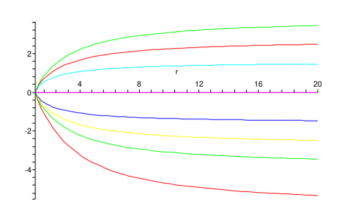
Figure 1: $\phi(r)$ vs. $r$, where the numerical coefficients are $r_{H}=1,l^{2}=6$ for the effective potential $V_{eff}=2e^{\sqrt{3}\phi}+2e^{-\sqrt{3}\phi}$. Different curves represent different asymptotic values for $\phi_{\infty}$. The attractor point is $\phi_{0}=0$ at the horizon, $r_{H}=1$.

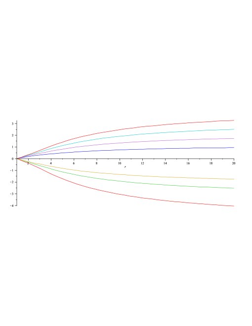
Figure 2: $\phi(r)$ vs. $r$, where the numerical coefficients are $r_{H}=1,l^{2}=6$ for the effective potential $V_{eff}=2e^{3\phi}+2e^{-3\phi}$. Different curves represent different asymptotic values for $\phi_{\infty}$. The attractor point is $\phi_{0}=0$ at the horizon, $r_{H}=1$.

3 AdS attractors with higher derivatives

The process of compactification of the string theory from higher to lower dimensions introduces scalar fields (moduli/dilaton) which are coupled to curvature invariants. We prove the existence of the attractor mechanism even in the presence of higher derivatives terms. For simplicity, we consider just $R^{2}$ corrections which appear in bosonic string theory but we expect to reach similar conclusions for more interesting case of the $R^{4}$ corrections.

3.1 Equations of motion for Gauss-Bonnet gravity

We add the most general $R^{2}$ correction with general scalar coupling to our previous action. The action is given by:

$$S=S_{0}+S_{corr}$$ (52)

where

$$S_{corr}=\frac{1}{\kappa^{2}}\int d^{5}x\sqrt{-g}\bigg{[}G_{1}(\phi_{i})R^{2}+G_{2}(\phi_{i})R_{\mu\nu}R^{\mu\nu}+G_{3}(\phi_{i})R_{\mu\nu\alpha\beta}R^{\mu\nu\alpha\beta}\bigg{]}$$

From now on we focus on $R^{2}$ corrections which form the Gauss-Bonnet Lagrangian

$$L_{GB}=R^{2}-4R_{\mu\nu}R^{\mu\nu}+R_{\mu\nu\alpha\beta}R^{\mu\nu\alpha\beta}.$$ (53)

that correspond to $G_{2}=-4G_{1},G_{3}=G_{1}$ in the above most general action. The equations of motion for the gauge fields do not change, while the scalar and three Einstein equations are modified by the Gauss-Bonnet term. Now we are again interested in static, spherically symmetric black holes. Thus, we consider the same ansatz as in the previous section for the gauge fields and the following ansatz for the metric:

$$ds^{2}=-a(r)^{2}dt^{2}+c(r)^{-2}dr^{2}+b(r)^{2}d\Omega_{3}^{2}$$ (54)

Then all the equations can be obtained from the following one-dimensional action (see the appendix for details):

$$S_{1-dim}= \frac{\pi}{4G_{N}}\int dr\bigg{[}3b^{2}b^{\prime}a^{\prime}c+\frac{3ab}{c}(1-b^{\prime 2}c^{2})+6abcb^{\prime 2}-\frac{1}{2}ab^{3}c\phi^{\prime 2}-\frac{a}{b^{3}c}V_{eff}(\phi)+\frac{6ab^{3}}{l^{2}c}$$ (56)

$$+12G(\phi)(ab^{\prime 3}c^{2}c^{\prime}+a^{\prime}b^{\prime}c+ab^{\prime 2}b^{\prime\prime}c^{3})-12G^{\prime}(\phi)(a^{\prime}bb^{\prime 2}c^{3}-a^{\prime}bc-ab^{\prime}c)\bigg{]}$$

After a little algebra, choosing the gauge $a=c$, the Einstein equations can be written as

$$\phi^{\prime 2}+3\frac{b^{\prime\prime}}{b^{3}}\left(b^{2}+4G(\phi_{i})(1-a^{2}b^{\prime 2})-8G^{\prime}(\phi_{i})a^{2}bb^{\prime}\right)+\frac{12G^{\prime\prime}(\phi_{i})}{b^{2}}(1-a^{2}b^{\prime 2})=0$$ (57)

(58)

$$4(-1+a^{2}b^{\prime 2})+(a^{\prime 2}+aa^{\prime\prime})b^{2}+ab(7a^{\prime}b^{\prime}+2ab^{\prime\prime})-\frac{12b^{2}}{l^{2}}$$ (59)

$$+\frac{4G(\phi_{i})}{b}{\mathcal{G}}_{1}-\frac{4G^{\prime}(\phi_{i})}{b}{\mathcal{G}}_{2}+4G^{\prime\prime}(\phi_{i})(a^{2}-a^{4}b^{\prime 2}-2a^{3}a^{\prime}bb^{\prime})=0$$ (60)

(61)

$$-1+aa^{\prime}bb^{\prime}+a^{2}b^{\prime 2}-\frac{1}{6}a^{2}b^{2}\phi^{\prime 2}+\frac{V_{eff}}{3b^{4}}-\frac{2b^{2}}{l^{2}}+\frac{4G(\phi_{i})}{b}(aa^{\prime}b^{\prime}-a^{3}a^{\prime}b^{\prime 3})$$ (62)

$$-\frac{4G^{\prime}(\phi_{i})}{b}(3a^{3}a^{\prime}bb^{\prime 2}-aa^{\prime}b-a^{2}b^{\prime}+a^{4}b^{\prime 3})=0$$ (63)

where

$${\mathcal{G}}_{1} = (1-a^{2}b^{\prime 2})(3aa^{\prime}b^{\prime}+aa^{\prime\prime}b)+a^{\prime 2}b(1-3a^{2}b^{\prime 2})-2a^{3}a^{\prime}bb^{\prime}b^{\prime\prime}$$ (64)

$${\mathcal{G}}_{2} = 6a^{2}a^{\prime 2}b^{2}b^{\prime}-3a^{2}b^{\prime}(1-a^{2}b^{\prime 2})-5aa^{\prime}b(1-3a^{2}b^{\prime 2})$$ (65)

$$+2a^{3}a^{\prime\prime}b^{2}b^{\prime}+2a^{3}a^{\prime}b^{2}b^{\prime\prime}+2a^{4}bb^{\prime}b^{\prime\prime}\;\;\;\;\;\;\;$$

and the equations of motion of scalar fields are given by

$$\partial_{r}(a^{2}b^{3}\partial_{r}\phi_{i}) = \frac{\partial_{i}V_{eff}}{b^{3}}-12\partial_{i}G\;\bigg{[}-a^{\prime 2}b+3a^{2}a^{\prime 2}bb^{\prime 2}-a(ab^{\prime\prime}+2a^{\prime}b^{\prime}+a^{\prime\prime}b)$$ (66)

$$+a^{3}b^{\prime}\bigg{(}(ab^{\prime\prime}+a^{\prime\prime}b)b^{\prime}+a^{\prime}(2b^{\prime 2}+2bb^{\prime\prime})\bigg{)}\bigg{]}$$

3.2 Zeroth order solution

Consider constant scalar fields $\phi_{i}=\phi_{i0}$. Then, equation ( 57 ) can be solved by

$$b(r)=r$$ (67)

Solving equations (57) and (62) for a double horizon (extremal) solution gives (see the Appendix for details)

$$a^{2}(r)=1+\frac{r^{2}}{4G_{0}}-\frac{r^{2}}{4G_{0}}\sqrt{1-\frac{8G_{0}}{l^{2}}+\frac{16G_{0}(G_{0}+r_{H}^{2}+\frac{3r_{H}^{4}}{2l^{2}})}{r^{4}}-\frac{8G_{0}r_{H}^{4}(1+\frac{2r_{H}^{2}}{l^{2}})}{r^{6}}}$$ (68)

where $G_{0}=G(\phi_{0i})$. Notice that in this case it is easier to solve the Hamiltonian constraint (62) than the equations of motion (as was done in section 2), since the equations of motion contain complicated second order derivative terms. Using the solutions for $a$ and $b$, the dilaton equation (66) becomes $\partial_{i}W(\phi_{i})|_{\phi_{i0}}=0$, where

$$W(\phi_{i})=V_{eff}(\phi_{i})+12r_{H}^{4}(1+\frac{3r_{H}^{2}}{l^{2}})\ln\left(1+\frac{4G(\phi_{i})}{r_{H}^{2}}\right)$$ (69)

is the analogue of the ”effective potential” when we add the Gauss-Bonnet correction.

The conditions for having attractor solutions are

$$\partial_{i}W(\phi_{i})|_{\phi_{i0}}=0$$ (70)

where

$$\tilde{M}_{ij}=\frac{1}{2}\partial_{i}\partial_{j}W(\phi_{i0})$$ (71)

have positive eigenvalues.

To find the entropy, we write equation (62) for the solution (67) and (68) at horizon $r=r_{H}$ and we get

$$-1+\frac{V_{eff}}{3r_{H}^{4}}-\frac{2r_{H}^{2}}{l^{2}}=0$$ (72)

Solving the algebraic equations (70) and (72) together, gives $r_{H}$ and $\phi_{i0}$ in terms of the charges carried by black hole. The entropy is obtained from the entropy function, by adding $-2\pi\int_{S^{3}}{\cal L}_{GB}$ to it, for the metric in (24).

$$S_{BH}=\frac{1}{2G_{N}}\pi^{2}r_{H}^{3}(1+\frac{12G_{0}}{r_{H}^{2}})=8\pi^{3}r_{H}^{3}(1+\frac{12G_{0}}{r_{H}^{2}})$$ (73)

3.3 First order solution

Starting with first order perturbation theory

$$\delta\phi_{i}=\phi_{i}-\phi_{i0}=\epsilon\phi_{i1}$$ (74)

where $\epsilon$ is a small parameter we use to organize the perturbation theory. The first correction to the scalars $\phi_{i}$ satisfies the equation

$$\partial_{r}(a^{2}b^{3}\partial_{r}\phi_{i1})=\frac{\beta_{i}^{2}}{b_{0}^{3}}\phi_{i1}$$ (75)

where $\beta_{i}^{2}$ is the eigenvalue for the matrix $2\tilde{M}_{ij}$. We are interested in a solution which does not blow up at the horizon $r=r_{H}$. This gives the following solution near the horizon

$$\phi_{i1}\simeq c_{1i}(1-\frac{r_{H}}{r})^{\gamma_{i}}$$ (76)

where $\gamma_{i}$ are positive roots of

$$\gamma_{i}(\gamma_{i}+1)=\frac{\beta_{i}^{2}}{4r_{H}^{4}}(1+\frac{4G_{0}}{r_{H}^{2}})(1+\frac{3r_{H}^{2}}{l^{2}})^{-1}$$ (77)

Asymptotically (as $r\rightarrow\infty$) $\phi_{i1}$ takes a constant value, $c_{1i}$ — however $\phi_{i1}$ is vanishing at the horizon and the value of the scalar is fixed at $\phi_{i0}$ regardless of its value at infinity.

3.4 Higher order solution

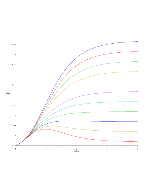
Figure 3: $\phi(r)$ vs. $\log(r)$, where numerical coefficients for the potentials are $g_{2}=1/9,v_{2}=2,v_{0}=4$ and $g_{0}=1/4$. Different curves represent different asymptotic values for $\phi_{\infty}$. The attractor point is $\phi_{0}=0$ at the horizon, $r_{H}=1$.

The analysis of the higher order solution is quite similar to the previous section. However it is rather difficult to solve the resulting differential equations analytically even in the second order. But as we will see below we can still solve our differential equations approximately order by order.

Without loss of generality, here we just consider the case with a single scalar field. All results can be simply generalized to the multi-scalar case. We can expand the solution in terms of the small parameter $x=r-r_{H}$ as a Frobenius series as follows

$$a(r) = \;(x+x^{\gamma_{1}}\;\sum_{n=2}^{\infty}a_{n}x^{n}),$$ (78)

$$b(r) = \;\frac{r_{H}}{1-x}\;(1+x^{\gamma_{2}}\sum_{n=1}^{\infty}b_{n}x^{n}),$$ (79)

$$\phi(r) = \;(\phi_{0}+x^{\gamma_{3}}\;\sum_{n=1}^{\infty}\phi_{n}x^{n}),$$ (80)

We also take a common $\gamma_{i}\equiv\gamma$ for all the solutions and write the series as:

$$\phi(r) = \phi_{0}+Kx^{\gamma}+\cdots,$$ (81)

$$a(r) = x+a_{1}x^{\gamma+1}+\cdots,$$ (83)

$$b(r) = r(1+b_{1}x^{\gamma}+\cdots).$$

We also consider Taylor series expansions for $V_{eff}(\phi)$ and $G(\phi)$ as follows,

$$V_{eff}(\phi) = v_{0}+v_{1}(\phi-\phi_{0})+\frac{1}{2}v_{2}(\phi-\phi_{0})^{2}+\cdots,$$ (85)

$$G(\phi) = g_{0}+g_{1}(\phi-\phi_{0})+\frac{1}{2}g_{2}(\phi-\phi_{0})^{2}+\cdots\>.$$ (86)

By a careful investigation near the horizon, for the lowest power of $x$ which is $x^{\gamma}$, one can solve the set of equations as we did in the previous subsection and find the non-trivial solutions (from (77), (72) and (71))

$$\gamma = \frac{1}{2}\left(-1+\sqrt{1+\frac{\beta^{2}}{r_{H}^{4}}(1+\frac{4g_{0}}{r_{H}^{2}})(1+\frac{3r_{H}^{2}}{l^{2}})^{-1}}\right),$$ (87)

$$v_{0}=3r_{H}^{4}+\frac{6r_{H}^{6}}{l^{2}},\;\;\;\;\;\;$$ (88)

with $v_{1}=g_{1}=a_{1}=b_{1}=0$ and

$$\beta^{2}=v_{2}+\frac{48g_{2}r_{H}^{4}(1+\frac{3r_{H}^{2}}{l^{2}})}{r_{H}^{2}+4g_{0}}$$ (89)

However, $v_{2}$, $g_{2}$ and $K$ are undetermined to this order. The second equation in (88) is the extremum condition for $W$ which gives the attractor value $\phi_{0}$ at the horizon. Notice that we are faced with an extra condition $g_{1}=0$, which indicates that $G$, $V_{eff}$ and $W$ are at their extremum at the horizon, simultaneously. Such a case is the only situation where a non-integer $\gamma$ can be found. Otherwise we have to choose $\gamma=0$ for $g_{1}\neq 0$. The regularity condition for $\phi$ indicates that $\gamma$ should be non-negative and it in turn gives $\beta^{2}>0$, or

$$v_{2}+\frac{48g_{2}r_{H}^{4}(1+\frac{3r_{H}^{2}}{l^{2}})}{r_{H}^{2}+4g_{0}}\geq 0\;.$$ (90)

This again means that $W_{H}$ is minimum at its extremum point $\phi_{0}$. Higher order terms can be derived in a similar fashion. The important point is that, due to the non-linear nature of equations, they are a mixture of different powers of $\gamma$, like $x^{n\gamma}$ as well as $x^{n\gamma+m}$. To order these powers, we assume $0<\gamma<1$. Then the next leading term would be $x^{2\gamma}$. For higher order terms, since $\gamma$ is already known from the first order result (87), we can determine whether the next order is $x^{3\gamma}$ or $x^{\gamma+1}$. For small enough $\gamma$, it shows that we are generating a power series, $x^{n\gamma}$ as argued in [17]. Notice that in contrast to the analysis of the previous section, here we considered all the equations simultaneously. This first means that, in principle, we are taking the backreaction into account. Secondly, we are dealing with a higher derivative theory, besides the Klein-Gordon equation for the $\phi$ field. Other equations also involve the second derivative of $\phi$ and are important in the dynamics of $\phi$. So, they should be investigated as well. To avoid quoting lengthy results, we demonstrate our results for a numerical simulation in figure 3.

4 Embedding in string theory: attractor horizons and moduli ‘flow’

In this section we present some physical interpretations of our results in the context of the AdS/CFT correpondence. After constructing the embedding in string theory, we consistently interpret the moduli flow in the bulk as a ‘holographic’ RG flow and construct the $c$-function. The attractor horizon has spherical topology and corresponds to an IR fixed point.

4.1 Holographic RG flow

We start by reviewing some known useful facts about the RG flow — we discuss the RG flow within the AdS/CFT correspondence and then we will interpret the moduli flow as a ‘holographic’ RG flow in the bulk of AdS spacetime.

The RG equation of a system (represented by its initial set of coupling constants) describes a trajectory (‘flow’) in the coupling constants space. The set of all such trajectories generated by different initial sets of coupling constants define the RG flow in the coupling constants space. In general it is found that such a trajectory is attracted to a fixed point that is a functional attractor for the flow. The behaviour within the functional attractor is then determined by the $\beta$-function for the relevant couplings. In string theory the couplings are identified with the moduli space of the theory under consideration.

The AdS/CFT correspondence is referred to as a duality since the supergravity (closed string) description of D-branes and the field theory (open string) description are different formulations of the same physics. This way, the infrared (IR) divergences of quantum gravity in the bulk are equivalent to ultraviolet (UV) divergences of the dual field theory living on the boundary. A remarkable property of the AdS/CFT correspondence is that it works even far from the conformal regime. Conformal field theories in various dimensions correspond to $AdS_{d+1}\times X_{q}$ gravitational theories. But one can also have cases that interpolate between asymptotically AdS spaces at the boundary and in the middle of the bulk, that are naturally interpreted as two conformal points of a dual QFT. Any hypersurface of constant radius in the bulk of AdS should have a field theory dual and the radial coordinate is consistently interpreted as the energy scale in the field theory. The RG ‘trajectory’ then allows us to define the UV and the IR limits of a given QFT and in the dual to interpret the ‘radial’ flow as a holographic RG flow. At a critical point a system can be regarded as scale invariant due to the violent critical fluctuations of the order parameter which lack any characteristic length and time scale. Thus, in the AdS/CFT context, the CFT on the boundary is the UV fixed point of a QFT in the bulk. Using the gravity side of the correspondence (deformations of AdS) one can obtain holographic RG flows corresponding to non-conformal field theories.

In [28], the Hamilton-Jacobi equations of canonical gravity were used to obtain first-order differential equations from the supergravity equations of motion and to derive the holographic RG flow. Specifically, the authors of [28] studied an action of scalar fields coupled to gravity with a non-trivial potential for the scalars:

$$S_{\rm loc}\,[\,\phi\,,\,g\,]\,=\;\int\!\!\sqrt{g}\,\Bigl{(}V(\phi)+R\,+\frac{1}{2}\partial^{\mu}\phi^{i}g_{ij}(\phi)\,\partial_{\mu}\phi^{j}\Bigr{)}$$ (91)

The first order equations of motion can be written as

$$\dot{\phi}^{i}=g^{ij}\partial_{j}U,\qquad\dot{g}_{\mu\nu}=-\frac{1}{3}U(\phi)g_{\mu\nu}$$ (92)

and the scalar potential $V(\phi)$ is related to ‘superpotential’ $U(\phi)$ by

$$V=\frac{1}{3}U^{2}-\frac{1}{2}\partial_{i}U\,g^{ij}\partial_{j}U$$ (93)

The identification of the holographic RG flow with the field theory local RG flow expressing how Weyl symmetry is broken allows to construct a holographic $c$-function and also the $\beta$-function. The solutions of this theory are BPS domain walls (${\cal N}=1$ supersymmetric kinks in the radial direction) and the flow is between different AdS spaces, which correspond to different ground states of the 5 dimensional ${\cal N}=8$ gauged supergravity.

However, the attractor mechanism appears in a slightly different context: the moduli potential is trivial (a constant) and instead the gauge fields in the bulk are turned on. There is an induced effective potential for the moduli due to the non-trivial coupling between moduli and the form fieds. The non-BPS flow is now between the boundary of an $AdS_{5}$ (UV region) and the horizon of the extremal black hole (IR region). For the extremal black hole solution, we have the usual $AdS_{5}$, but a trivial flow. For a large enough perturbation $\delta\phi_{i}$, we can reach another $AdS_{5}$ vacuum, and then we will have a holographic flow between the new $AdS_{5}$ and the horizon of the extremal black hole.

There is an enhanced symmetry $AdS_{2}\times S^{3}$ in the near-horizon limit and so the flow is still between two AdS vacua, albeit with different dimensionality — however,the supersymmetry can be broken in the bulk. The breaking of supersymmetry is not problematic, as one can have a nonsupersymmetric RG flow between conformal points in a supersymmetric theory, but the change from $AdS_{5}$ to $AdS_{2}\times S^{3}$ is more puzzling, however we will analyze it in the next subsection.

At this point it is useful, though, to present some computational details on solutions which interpolate between two critical points and emphasize similarities between the kink solutions with and without horizons.

First, let us discuss a simple model with a single bulk scalar field coupled to gravity (see e.g., [31, 32]). We describe a domain wall solution that interpolates between two AdS spaces with different radii. The scalar non-linear equation of motion is well approximated by a linear solution near a critical point — let us consider a quadratic approximation given by:

$$V(\phi)\simeq V(\phi_{0})+\frac{1}{2}\beta^{2}\phi_{1}^{2}\,,\hskip 56.9055pt\phi_{1}=\phi-\phi_{0}$$ (94)

thus the corresponding solution is (here $r$ is a coordinate in the AdS space at infinity defined as in (112))

$$\phi_{1}(r)=Ar^{(\Delta-4)}+Br^{-\Delta}\,,\hskip 56.9055pt\Delta=2+\sqrt{4+\beta^{2}l^{2}}$$ (95)

The UV point corresponds to the boundary ($r\rightarrow\infty$) and the fluctuation should die off ($\phi(r)\rightarrow\phi_{0}^{UV}$). The solution is then given by

$$\phi(r)=\phi_{0}^{UV}+\phi_{1}^{UV}\approx\phi_{0}^{UV}+Ar^{(\Delta^{UV}-4)}+Br^{-\Delta^{UV}}$$ (96)

with the constraint $2<\Delta^{UV}<4$ that is equivalent with a negative mass², $\beta^{2}<0$. Thus the critical point is a local maximum given by $V(\phi_{0}^{UV})$ and the dual QFT is a relevant deformation of an UV CFT that is living on the boundary region of the domain wall solution.

The IR point corresponds to a region deep in the bulk ($r\rightarrow 0$) and the corresponding critical point should be a minimum. The solution is again given by

$$\phi(r)=\phi_{0}^{IR}+\phi_{1}^{IR}\approx\phi_{0}^{IR}+Cr^{(\Delta^{IR}-4)}+Dr^{-\Delta^{IR}}$$ (97)

except that $\Delta^{IR}>4$ that correponds to a positive mass², $\beta^{2}>0$ — that imposes a further constraint, namely $D=0$ (this term would be divergent). Thus, as expected from RG flow properties, the domain wall approaches the IR region in the bulk with the scaling rate of an irrelevant operator of dimension $\Delta^{IR}>4$.

We are now ready to understand the case of interest, a black hole in AdS. In this case the deep IR region corresponds to the black hole horizon. By imposing the attractor conditions, the horizon should be a stable minimum of the effective potential. It is interesting to observe that there also are two solutions in the near horizon limit, but the existence of a regular horizon forces us to discard the divergent mode. Therefore, the attractor horizon describes the IR point of an RG flow and corresponds to a deformation of a CFT by an irrelevant operator (see, also, [17]). For completness, we present the behaviour of the first order solution at the AdS boundary. Consider the equations (36) and (41) at large $r$ — (41) becomes

$$\partial_{r}(\frac{r^{5}}{l^{2}}\partial_{r}\phi_{i1})=\frac{\beta_{i}^{2}}{r^{3}}\phi_{i1}$$ (98)

Let us define $y\equiv\frac{\beta_{i}l}{3r^{3}}$, then for large r we obtain

$$\phi_{i1}(r)=c_{1}y^{\frac{2}{3}}I_{\frac{2}{3}}(y)+c_{2}y^{\frac{2}{3}}I_{-\frac{2}{3}}(y)$$ (99)

where $c_{1}$ and $c_{2}$ are arbitrary constants and $I_{\nu}$ stands for a modified Bessel function.

In conclusion it is very tempting to interpret the moduli flow as the holographic RG flow in the bulk — we will make these ideas more concrete in the following by constructing explicitly the string theory embedding of our system and studying its $c$-function.

4.2 String theory embedding

We have been analyzing asymptotically $AdS_{5}$ solutions until now. In order to talk about AdS/CFT however we need to have 10 dimensional IIB supergravity solutions. So we need to understand whether we can embed the extremal black holes in 10 dimensions via a consistent truncation. The extremal black holes can be embedded in 5 dimensional ${\cal N}=8$ gauged supergravity, and therefore are in the same class as the solutions of [31]. It is believed that the full ${\cal N}=8$ 5 dimensional gauged supergravity is a consistent truncation of 10 dimensional IIB supergravity as in the 4 dimensional [33] and 7 dimensional [34] cases, though until now only subsets of it have been obtained as consistent truncations. For the case of extremal black holes however, we have not only an embedding in 10 dimensional IIB supergravity, but we can even obtain it as the near horizon limit of a system of D-branes [6].

The extremal RNAdS solution is a special case of the 3-charge black holes in [35, 6], with $H_{1}=H_{2}=H_{3}\equiv H$. The general (non-extremal) solution is

$$ds_{5}^{2}=-(H_{1}H_{2}H_{3})^{-2/3}f\;dt^{2}+(H_{1}H_{2}H_{3})^{1/3}(f^{-1}dr^{2}+r^{2}d\Omega_{3,k}^{2});$$

$$X_{i}=H_{i}^{-1}(H_{1}H_{2}H_{3})^{1/3},\;\;\;A^{i}=\sqrt{k}(1-H_{i}^{-1})\coth\beta_{i}dt$$ (100)

where

$$f=k-\frac{\mu}{r^{2}}+g^{2}r^{2}(H_{1}H_{2}H_{3}),\;\;\;H_{i}=1+\frac{\mu\sinh^{2}\beta_{i}}{kr^{2}}$$ (101)

and $k=1,0,-1$ corresponds to having $S^{3},T^{3}$ or $H^{3}$ foliations, so the case studied here corresponds to $k=1$. If $H_{1}=H_{2}=H_{3}=H$ (thus $\beta_{i}=\beta$), then $X_{i}$=constant=$X$. The change of coordinates $\tilde{r}^{2}=Hr^{2}=r^{2}+\mu\sinh^{2}\beta$ brings us to our metric in $\tilde{r}$ coordinates, since $dr^{2}=Hd\tilde{r}^{2}$ and

$$H^{-2}f=g^{2}\tilde{r}^{2}+1-\frac{\mu(2\sinh^{2}\beta_{i}+1)}{\tilde{r}^{2}}+\frac{\mu^{2}\sinh^{2}\beta_{i}\cosh^{2}\beta_{i}}{\tilde{r}^{4}}$$ (102)

is identified with $a^{2}$, if we have

$$g^{2}=\frac{1}{l^{2}};\;\;\sinh^{2}\beta=-\frac{1}{2}+\frac{1}{2}\sqrt{1+\frac{1+2r_{H}^{2}/l^{2}}{r_{H}^{2}/l^{2}(1+9r_{H}^{2}/4l^{2})}};\;\;\;\mu=\frac{r_{H}^{2}(2+3r_{H}^{2}/l^{2})}{\sqrt{1+\frac{1+2r_{H}^{2}/l^{2}}{r_{H}^{2}/l^{2}(1+9r_{H}^{2}/4l^{2})}}}$$ (103)

and then we also get $A_{i}=qdt/\tilde{r}^{2}$.

The 10 dimensional embedding of the extremal RNAdS solution is obtained from the 10 dimensional reduction ansatz used in [6], namely

$$ds_{10}^{2}=\sqrt{\tilde{\Delta}}ds_{5}^{2}+\frac{1}{g^{2}\sqrt{\tilde{\Delta}}}\sum_{i=1}^{3}X_{i}^{-1}(d\mu_{i}^{2}+\mu_{i}^{2}(d\phi_{i}+gA_{i})^{2})$$ (104)

where $\tilde{\Delta}=\sum_{i=1}^{3}X_{i}\mu_{i}^{2}$ and

$$d\Omega_{5}^{2}=\sum_{i=1}^{3}d\mu_{i}^{2}+\mu_{i}^{2}d\phi_{i}^{2};\;\;\;\mu_{1}=\sin\theta;\;\;\mu_{2}=\cos\theta\sin\psi;\;\;\;\mu_{3}=\cos\theta\cos\psi$$ (105)

is the 5-sphere metric. It is important to notice that each angular momentum becomes a charge after KK reduction on $S^{5}$ — this resembles the KK reduction on a circle when the momentum on the circle becomes the electric charge (the circle fibration will give the magnetic charge).

In our case, since $X_{i}=X$=1, $\tilde{\Delta}=X$, and $1/g^{2}=l^{2}$ we get

$$ds_{10}^{2}=ds_{5}^{2}+l^{2}\sum_{i=1}^{3}[d\mu_{i}^{2}+\mu_{i}^{2}(d\phi_{i}+gA_{i})^{2}]$$ (106)

so the extremal RNAdS is embedded (up to a constant rescaling) by just adding a sphere of radius $l$, squashed by the gauge field, i.e. rotating on this 5-sphere.

Since we have a 10 dimensional IIB supergravity solution, we can safely use AdS/CFT. But it would be useful to have also a D-brane solution that gives the above solution in the decoupling limit.

It is known that the general RNAdS black hole embeds to the above 10 dimensional metric, which corresponds to adding a chemical potential for the R charge in AdS/CFT [36] . It is also known how to obtain the $k=0$ (torus foliation) AdS black holes from the decoupling limit of rotating D3-branes [6]. But a minimal change is needed to obtain the $k=1$ black holes considered here.

The D3 branes rotating with 3 angular momenta $l_{i},i=1,2,3$ in 3 different directions have the metric

$$ds^{2}=H^{-1/2}(-(1-\frac{2m}{r^{4}\Delta})dt^{2}+dx_{1}^{2}+dx_{2}^{2}+dx_{3}^{2})+H^{1/2}\left[\frac{\Delta dr^{2}}{H_{1}H_{2}H_{3}-2m/r^{4}}\right.$$

$$\left.+r^{2}\sum_{i=1}^{3}H_{i}(d\mu_{i}^{2}+\mu_{i}^{2}d\phi_{i}^{2})-\frac{4m\cosh\alpha}{r^{4}H\Delta}dt\sum_{i=1}^{3}l_{i}\mu_{i}^{2}d\phi_{i}+\frac{2m}{r^{4}H\Delta}(\sum_{i=1}^{3}l_{i}\mu_{i}^{2}d\phi_{i})^{2}\right]$$ (107)

where

$$\Delta=H_{1}H_{2}H_{3}\sum_{i=1}^{3}\frac{\mu_{i}^{2}}{H_{i}};\;\;\;H=1+\frac{2m\sinh^{2}\alpha}{r^{4}\Delta};\;\;\;H_{i}=1+\frac{l_{i}^{2}}{r^{2}}$$ (108)

In our case, $l_{1}=l_{2}=l_{3}\equiv l_{0}$, so $H_{1}=H_{2}=H_{3}\equiv h$, and $\Delta=h^{2}$. Making again the change of variables $\tilde{r}^{2}=r^{2}+l_{0}^{2}$ we get $r^{4}\Delta=\tilde{r}^{4}$ and

$$ds^{2}=H^{-1/2}[-(1-\frac{2m}{\tilde{r}^{4}})dt^{2}+dx_{1}^{2}+dx_{2}^{2}+dx_{3}^{2}]+H^{1/2}\left[\frac{d\tilde{r}^{2}}{1-\frac{2m}{\tilde{r}^{4}}+\frac{2ml_{0}^{2}}{\tilde{r}^{6}}}\right.$$

$$\left.+\tilde{r}^{2}d\Omega_{5}^{2}-\frac{4ml_{0}\cosh\alpha}{\tilde{r}^{4}H}dt\sum_{i=1}^{3}\mu_{i}^{2}d\phi_{i}+\frac{2ml_{0}^{2}}{\tilde{r}^{4}H}(\sum_{i=1}^{3}\mu_{i}^{2}d\phi_{i})^{2}\right]$$ (109)

where $H=1+2m\sinh^{2}\alpha\;\tilde{r}^{-4}$.

The decoupling limit is obtained via the rescalings

$$m=\epsilon^{4}m^{\prime};\;\;\;\sinh\alpha=\epsilon^{-2}\sinh\alpha^{\prime};\;\;\;r=\epsilon\;r^{\prime};\;\;\;x^{\mu}=\epsilon^{-1}x^{\prime\mu};\;\;\;l_{i}=\epsilon l_{i}^{\prime}$$ (110)

followed by $\epsilon\rightarrow 0$ and dropping the primes. One then gets (104) with

$$d\Omega_{3,k}^{2}=d\vec{y}\cdot d\vec{y};\;\;\;\vec{y}=g\vec{x};\;\;\;\frac{1}{g^{2}}=\sqrt{2m}\sinh\alpha;\;\;\;\mu=2mg^{2};\;\;\;l_{i}^{2}=\mu\sinh^{2}\beta_{i}$$ (111)

But notice that if in the final metric (104) we change from $k=0$ to $k=1$, replacing $d\vec{y}\cdot d\vec{y}$ with $d\Omega_{3}^{2}$, and correspondingly we add $1$ inside $f$, we can still obtain the metric from the decoupling limit of the same D3 brane metric (107), with an infinitesimal perturbation. Indeed, the decoupling limit involves $x^{\mu}=\epsilon^{-1}x^{\prime\mu}$, which now we can understand as rescaling the radius in $R^{2}d\Omega_{3}^{2}$ by $R=R^{\prime}/\epsilon$. Since after the rescaling we want to have $R^{\prime}=1$, it means initially $R=1/\epsilon\rightarrow\infty$, thus a sphere of a very large radius, still approximated by a plane. Moreover, the addition of the $+1$ in $f$ implies the addition of $(g^{2}r^{2}H_{1}H_{2}H_{3})^{-1}$ to $1-\frac{2m}{r^{4}\Delta}$ in the coefficient of $dt^{2}$ and of $1/(g^{2}r^{2})$ ($=\sqrt{2m}\sinh\alpha/r^{2}$) to $H_{1}H_{2}H_{3}-2mr^{-4}$ in the coefficient of $dr^{2}$. However, the same reasoning tells us that in order to get a finite result after the decoupling limit, these added terms need to be multiplied by $\epsilon^{2}\rightarrow 0$. In conclusion, we can actually also obtain the $k=1$ case (sphere foliation) from (107), with an infinitesimal perturbation.

So the extremal RNAdS metric with sphere foliation can be obtained as a consistent truncation of the near horizon limit of rotating D3 branes. Since the nonrotating case is dual to ${\cal N}=4$ Super Yang-Mills, the perturbed extremal RNAdS solution should correspond to adding a perturbation in the UV and obtaining an RG flow to a different (IR) conformal fixed point.

As we noticed however, there is an aparent discrepancy in dimensionality, namely we start with $AdS_{5}$ in the UV and get $AdS_{2}\times S^{3}$ in the IR, that seems problematic at first sight (for usual holographic flows we go between two different $AdS_{5}$’s). However, what is important for the conformal field theory is the global boundary of $AdS_{5}$ and $AdS_{2}\times S^{3}$, which in both cases is $R_{t}\times S^{3}$ (conformal to 4 dimensional flat space). Note that we have used throughout the sphere foliation of AdS space and the AdS space extremal black hole, where the metric at infinity is

$$ds^{2}\simeq-\frac{r^{2}}{l^{2}}dt^{2}+l^{2}\frac{dr^{2}}{r^{2}}+r^{2}d\Omega_{3}^{2}$$ (112)

for which the $R_{t}\times S^{3}$ boundary at $r\rightarrow\infty$ is actually parametrized by $t$ and $\Omega_{3}$ (and $r^{2}$ is taken out when we consider the conformal boundary). For the $AdS_{2}\times S^{3}$ near the horizon, the $S^{3}$ metric is $(r_{H}+\rho)^{2}d\Omega_{3}^{2}$ (here $\rho=r-r_{H}$), and the interpolation between $r^{2}$ and $r_{H}^{2}$ is done by $b(r)^{2}$, which does look indeed like a holographic flow between two dual RG fixed points. Notice then that the correct conformal radius of the two (dual) $\Omega_{3}$’s is given by $b^{\prime}(r)$, since it gives $1$ for the extremal black hole, both at the boundary and at infinity. This is what we want since in the extremal case the dual CFT does not change, and has conformal radius $1$.

In conclusion, in the case of a nontrivial holographic flow (perturbed extremal black hole) both the UV and IR correspond to 4 dimensional conformal field theories, which we expected, since we have a holographic flow of ${\cal N}=8$ 5 dimensional gauged supergravity, dual to an RG flow in 4 dimensions. A nontrivial holographic flow occurs if the perturbation $\delta\phi_{i}$ is large enough to produce a new $AdS_{5}$ vacuum. This is so, since an RG flow relates two conformal fixed points, and a small perturbation will get us away from the original $AdS_{5}$ vacuum.

The holographic RG flow is 10 dimensional, but reduces to the 5 dimensional flow upon the dimensional reduction on $S^{5}$ in (104). The sphere $S^{5}$ now plays a role, since its squashing (rotation) due to the gauge field $A_{i}$ is partly responsible for the flow (unlike previous cases, the flow is not solely governed by scalar fields, but is also governed by gauge fields).

Another important consequence of the embedding of the 5 dimensional extremal RNAdS solution into a rotating D3 solution is understanding the attractor mechanism from a different perspective. The 10 dimensional rotating D3 branes will presumably have their own attractor mechanism, i.e. a flow between the 10 dimensional flat space at infinity and the near horizon limit of the rotating D3 branes. One could conceivably then embed the 5 dimensional AdS space attractor mechanism discussed in this paper as the decoupling limit (110) of the attractor mechanism of the rotating D3 branes. We leave however the exploration of this possibility for further work.

4.3 c-function

We now turn to the calculation of the c-function. A c-function is a monotonic function that takes the value of the central charge of the UV fixed point in the UV and of the IR fixed point in the IR.

The central charge counts the number of massless degrees of freedom in the CFT (it counts the ways in which the energy can be transmitted). The coarse graining of a quantum field theory removes the information about the small scales, in other words there is a gradual loss of non-scale invariant degrees of freedom. Thus, for a QFT RG flow, there should exist a c-function that is decreasing monotonically from the UV regime (large radii in the dual AdS space) where it gives $c_{UV}$ to the IR regime (small radii in the gravity dual) of the QFT where it gives $c_{IR}$, a statement known as the c-theorem. A c-theorem for gauge theory that is living on the AdS boundary with topology $R\times S^{3}$ was constructed in [37].

In order to get the c-function we look for a monotonic function of $r$, $A(r)$, along the flow, and then the c-function is ${\mathcal{C}}(r)=A(r)^{n}$, such that

$$\frac{c_{UV}}{c_{IR}}=\frac{{\mathcal{C}}(r=\infty)}{{\mathcal{C}}(r=r_{H})}=\left(\frac{A(r=\infty)}{A(r=r_{H})}\right)^{n}$$ (113)

from which we find the appropriate power of $n$.

The monotonic function of $r$ along the flow is found from the Einstein equations. The right hand side of the Einstein equations is the energy momentum tensor, which should obey the weak (null) energy condition, $T_{\mu\nu}\xi^{\mu}\xi^{\nu}\geq 0$, with $\xi$ null. The weak energy condition (the GR equivalent of the positivity of local energy density) implies a second order inequality for the metric coefficients, that may sometimes be written as the positivity of the derivative of a function, thus extracting the monotonic function.

Consider the most general ansatz for the metric with spherical symmetry as follows

$$ds^{2}=-a(r)^{2}dt^{2}+\frac{dr^{2}}{c(r)^{2}}+b(r)d\Omega_{3}^{2}$$ (114)

The combination $R_{rr}-\frac{G_{rr}}{G_{tt}}R_{tt}$ of the Ricci tensor components gives

$$3\left(-\frac{b^{\prime\prime}}{b}-\frac{b^{\prime}c^{\prime}}{bc}+\frac{a^{\prime}b^{\prime}}{ab}\right)=g_{ij}\partial_{\mu}\phi^{i}\partial^{\mu}\phi^{j}=\phi^{\prime 2}$$ (115)

using (115), it is straightforward to see that

$${\mathcal{C}}(r)={\mathcal{C}}_{0}\;\frac{a^{3}}{b^{\prime 3}c^{3}}$$ (116)

is a monotonically increasing function of $r$ for any positive constant ${\mathcal{C}}_{0}$. Therefore for the unperturbed extremal solution ($a=c,b^{\prime}=1$), ${\mathcal{C}}(r)={\mathcal{C}}_{0}=$ constant, which is as it should be, since for the extremal solution there is no RG flow. For the perturbed extremal black hole, $a=c$, but $b^{\prime}\neq 1$, thus we get a nontrivial flow. The flow relates two different conformal fixed points if the perturbation is large enough to reach a new $AdS_{5}$ vacuum of ${\cal N}=8$ supergravity. Since $b^{\prime}(r)$ acts as the conformal radius of $S^{3}$, $c_{UV}/c_{IR}$ should indeed scale as $b^{\prime 3}$, hence the cubic power in ${\mathcal{C}}(r)$.

5 Discussion

In this paper, we have investigated the attractor mechanism in spaces with negative cosmological constant. A straightforward extension of the effective potential method [17] confirms that the attractor mechanism still occurs for 5-dimensional extremal black holes in AdS space. This is expected since the near-horizon geometry of five dimensional extremal charged black holes in AdS has the $SO(2,1)\times SO(4)$ isometry. The origin of the attractor mechanism is in the enhanced symmetry of the near-horizon geometry that contains the infinite long throat of $AdS_{2}$. The entropy function is constructed (on an $SO(2,1)\times SO(4)$ symmetric background) by taking the Legendre transform (with respect to electric charges) of the reduced Lagrangian evaluated at the horizon. By extremising the entropy function one obtains the equations of motion at the horizon and its extremal value corresponds to the entropy that is independent of the asymptotic data. However, if the entropy function has flat directions the extremum remains fixed but the flat directions will not be fixed by near horizon data and can depend on the asymptotic moduli. In this paper we also have shown the equivalence of the effective potential method and the entropy function in the near-horizon limit for extremal black holes in AdS.

In Section 3 we have studied the attractor mechanism in AdS space in the presence of higher derivative terms (we present explicit results for the Gauss-Bonet term). The analysis is more involved but we reached similar conclusions. The near-horizon geometry remains $AdS_{2}\times S^{3}$ even after adding $\alpha^{\prime}$ corrections — the radii of $AdS_{2}$ and $S^{3}$ receive corrections, but the geometry does not change (also see, e.g., [12, 39]). For the Gauss-Bonnet correction, in a background with asymptotic $AdS$ boundary condition, the regularity of scalar fields at the horizon is a sufficient (and obviously necessary) condition to have the attractor mechanism — regularity at the horizon restricts the effective potential $W$ to be at its minimum at the critical point that is equivalent with the fact that the near horizon geometry is $AdS_{2}\times S^{3}$.

Sen’s entropy function formalism was applied to extremal black holes in AdS in the presence of higher derivatives terms in [22]. The advantage of this method is that the higher derivatives terms can be incorporated easily, but the method can not be used to determine the properties of the solution away from the horizon. In this paper, we used the effective potential method (that is based on the equations of motion in the bulk) to prove the existence of the attractor mechanism in AdS space with higher derivatives.

When the scalar potential is not a constant, a general analysis of the attractor mechanism is difficult. The reason is that the right hand side of the equation of motion for the moduli (15) contains two terms: a term that depends of the effective potential and the other one depends on the scalar potential. Thus, there is a competition between these two terms in the bulk and this is why the analysis is difficult. In the near horizon limit both terms are present and if the near horizon geometry is still $AdS_{2}\times S^{3}$, then the entropy function formalsim can still be applied to compute the entropy. On the other hand the effective potential dies off at the boundary and the moduli at the bounday are fixed at the minimum of the scalar potential — the existence of a full solution from the horizon to the boundary is problematic in this case. However, within the AdS/CFT correspondence, the critical point of the potential at the boundary should be a a local maximum such that a relevant deformation in the ultraviolet CFT gives a new long distance realization of the field theory. Therefore a discussion of the attractor mechanism for a theory with a non-trivial moduli potential should be made case by case. On the other hand, we were able to completely study the attractor mechanism in AdS space for which the moduli potential is constant (related to the cosmological constant).

In Section 4 we provided some physical interpretations of our results in the context of the AdS/CFT correspondence. We interpreted the moduli flow as a holographic RG flow in the AdS bulk and constructed the corresponding c-function. Let us now discuss in detail these results.

It is well known that by using different foliations of AdS space one can describe boundaries that have different topologies affording the study of CFT on different backgrounds. We are interested in a foliation of AdS for which the boundary has the topology $R\times S^{3}$ — the black holes in this space have horizons with spherical topology. The diffeomorphisms in the bulk are equivalent with the conformal transformations in the boundary and the spherical boundary is related conformally to the flat boundary if the point at the infinity is added for the latter. In other words, the boundaries with different topologies are related by singular conformal transformations. Since the CFT is living on a boundary with the topology $R\times S^{3}$ there is an additional Casimir-type contribution to the total energy in accord with the expectations from quantum field theory in curved space [40] — the central charge is related to the Casimir energy in the boundary. In [37], a c-function (an off-shell generalization of the central charge) for an AdS space foliated by spherical slices was proposed.

For a supersymmetric flow the IR point is a naked singularity (the BPS limit of a RN-AdS black hole is different than its extremal limit and it has a naked singularity) — the analysis in [37] was done for only one gauge field. There is a similar situation in flat space: if we consider a theory with just one gauge field exponentially coupled to the dilaton, the extremal limit is a naked singularity. The non-trivial form field generates an effective potential for the dilaton, but this potential does not have a minimum. To obtain a stable minimum a second gauge field should be turned on and so in theories with more than one gauge field we expect non-singular BPS limits of extremal black holes in AdS. With just one gauge field, as in [37], we expect that the $\alpha^{\prime}$ corrections will play an important role and the naked singularity may be dressed by a horizon. Another way to avoid this problem may be that the flow is ending on the surface of a star and so the number of degrees of freedom is much smaller than in the case of a horizon, but still non-zero.

However, our case is different — we are interested in non-supersymmetric attractors in AdS for which the supersymmetry can be broken in the bulk. At a first look, the existence of a c-function seems problematic. This issue was addressed in [42] for attractor horizons in flat space (though, the physical interpretation of a c-function in flat space is less clear than in AdS) and is closely related with the existence of first order equations of motion. In [42] it was argued that the boundary conditions play an important role in the sense that the attractor boundary conditions restrict the allowed initial conditions to make the equations first order such that the solution at the horizon is regular. The definition of the c-function is best understood if we have a concrete string theory embedding.

We have shown that the extremal black hole becomes a 10 dimensional black hole solution rotating in the extra $S^{5}$ (we simply add a 5-sphere deformed by the gauge field). Also, we have seen that we can obtain this 10 dimensional metric as the decoupling limit of a system of rotating black D3 branes, even in the case we are interested in, of boundary topology $R\times S^{3}$ (sphere foliation of the AdS black hole). Now, we can safely interpret our results within AdS/CFT duality as in the following.

Since the AdS black hole is the dimensional reduction of the decoupling limit of a black D3-brane system, which has a flat asymptotic at 10 dimensional infinity, one could also try to understand the attractor mechanism by embedding in flat 10 dimensions. The rotating black D3-branes have a near horizon limit, which is however harder to understand because of the angular dependence. Therefore we can imagine defining an attractor mechanism for the rotating black D3-branes in flat 10 dimensional space, as in [14]. If the 10d horizon is an attractor, one could imagine taking a decoupling limit of the near horizon geometry, followed by dimensional reduction, and hopefully one would obtain the 5 dimensional attractor (horizon of the 5d AdS black hole), thus embedding the $AdS_{5}$ attractor mechanism in the usual attractor mechanism in flat 10 dimensions. The limits involved are however quite subtle, so we leave the details of this analysis for further work.

To define AdS/CFT, one looks at fluctuations in the gravity dual. A field in Lorentzian AdS space has two kinds of modes, normalizable and non-normalizabile. While the former corresponds to a state in the CFT, the non-normalizable mode corresponds to insertion of an operator in the boundary (a bulk field is the source for an operator in the QFT). So, if the boundary conditions are kept fixed and the bulk is modified (for example, black holes or gravitational waves) the objects in the bulk correspond to states in the boundary (certain operators acquire expectations values). An extremal black hole is a zero temperature state in the CFT. An operator deformation in the CFT will produce an interpolating flow in which the scalar moduli approach a maximum critical point at the (UV) boundary and a minimum at the (IR) black hole horizon.

We have shown that the attractor mechanism works also in AdS space, not only in flat space. However, the interpretation seems to be somewhat different. In flat space, the attractor mechanism means that the horizon values for the moduli of the extremal black hole are fixed and the entropy (the value of the entropy function at the minimum) depends only on the charges $q_{i}$. In $AdS_{5}$, a priori there is one more parameter in the entropy, $G_{N,5}/l^{3}$ ($l$ is the AdS radius), which varies continuosly. However, the correct interpretation of the moduli flow is as a 10 dimensional RG flow. Then, in string theory, $G_{N,5}=G_{N}/(R_{S^{5}})^{5}$ and $R_{S^{5}}=l,G_{N}=g_{s}^{2}(\alpha^{\prime})^{4}$, which means that $G_{N,5}/l^{3}=1/N^{2}$ is independent on any continous parameters. Therefore only after embedding in string theory the attractor mechanism is on the same footing as in flat space.

Appendix A The equations of motion for the $R^{2}$ term

For 5-dimensional, spherically symmetric, extremal Gauss-Bonnet black holes with a cosmological constant, we take the following ansatz for the metric:

$$ds^{2}=-a(r)^{2}dt^{2}+c(r)^{-2}dr^{2}+b(r)^{2}d\Omega_{3}^{2}$$ (117)

Then all the equations of motion including the Hamiltonian constraint are obtained by taking derivatives with respect to the metric components, gauge and scalar fields and choosing the gauge $a(r)=c(r)$ from the following one-dimensional action:

$$I=\frac{\pi}{8G_{N}}\int dr\frac{ab^{3}}{c}\bigg{[}R-c^{2}g_{ij}\partial_{r}\phi^{i}\partial_{r}\phi^{j}-\frac{2}{b^{6}}V_{eff}(\phi^{i})+\frac{12}{l^{2}}+G(\phi^{i})L_{GB}\bigg{]}$$ (118)

where

$$R=-\frac{2}{ab^{2}}\bigg{[}b^{2}c(a^{\prime}c)^{\prime}+3a(-1+c^{2}b^{\prime 2})+3bc(ab^{\prime}c)^{\prime}\bigg{]}$$ (119)

$$V_{eff}(\phi^{i})=f^{AB}(\phi^{i})Q_{A}Q_{B}$$ (120)

and

$$L_{GB}= R^{2}-4R_{\mu\nu}R^{\mu\nu}+R_{\mu\nu\alpha\beta}R^{\mu\nu\alpha\beta}$$

$$= \frac{24c}{ab^{3}}\bigg{[}-(ab)^{\prime}c^{\prime}+(ab^{\prime}+3a^{\prime}b)b^{\prime 2}c^{2}c^{\prime}-(ab^{\prime\prime}+a^{\prime}b^{\prime}+a^{\prime\prime}b)c$$ (121)

$$+\bigg{(}(ab^{\prime\prime}+a^{\prime\prime}b)b^{\prime}+a^{\prime}(b^{\prime 2}+2bb^{\prime\prime})\bigg{)}b^{\prime}c^{3}\bigg{]}$$

By varying the above full action with respect to each metric component, $a$, $b$ and $c$, and taking the gauge $a=c$, we obtain the following equations:

$$\phi^{\prime 2}+3\frac{b^{\prime\prime}}{b^{3}}\left(b^{2}+4G(\phi_{i})(1-a^{2}b^{\prime 2})-8G^{\prime}(\phi_{i})a^{2}bb^{\prime}\right)+\frac{12G^{\prime\prime}(\phi_{i})}{b^{2}}(1-a^{2}b^{\prime 2})=0$$ (122)

(123)

$$4(-1+a^{2}b^{\prime 2})+(a^{\prime 2}+aa^{\prime\prime})b^{2}+ab(7a^{\prime}b^{\prime}+2ab^{\prime\prime})-\frac{12b^{2}}{l^{2}}$$ (124)

$$+\frac{4G(\phi_{i})}{b}{\mathcal{G}}_{1}-\frac{4G^{\prime}(\phi_{i})}{b}{\mathcal{G}}_{2}+4G^{\prime\prime}(\phi_{i})(a^{2}-a^{4}b^{\prime 2}-2a^{3}a^{\prime}bb^{\prime})=0$$ (125)

(126)

$$-1+aa^{\prime}bb^{\prime}+a^{2}b^{\prime 2}-\frac{1}{6}a^{2}b^{2}\phi^{\prime 2}+\frac{V_{eff}}{3b^{4}}-\frac{2b^{2}}{l^{2}}+\frac{4G(\phi_{i})}{b}(aa^{\prime}b^{\prime}-a^{3}a^{\prime}b^{\prime 3})$$ (127)

$$-\frac{4G^{\prime}(\phi_{i})}{b}(3a^{3}a^{\prime}bb^{\prime 2}-aa^{\prime}b-a^{2}b^{\prime}+a^{4}b^{\prime 3})=0$$ (128)

where

$${\mathcal{G}}_{1} = (1-a^{2}b^{\prime 2})(3aa^{\prime}b^{\prime}+aa^{\prime\prime}b)+a^{\prime 2}b(1-3a^{2}b^{\prime 2})-2a^{3}a^{\prime}bb^{\prime}b^{\prime\prime}$$ (129)

$${\mathcal{G}}_{2} = 6a^{2}a^{\prime 2}b^{2}b^{\prime}-3a^{2}b^{\prime}(1-a^{2}b^{\prime 2})-5aa^{\prime}b(1-3a^{2}b^{\prime 2})+2a^{3}b^{2}(a^{\prime}b^{\prime})^{\prime}+2a^{4}bb^{\prime}b^{\prime\prime}\;\;\;\;\;$$ (131)

Note that differentiating the action with respect to $c(r)$ gave us the Hamiltonian constraint.
The equation of motion for scalar fields is obtained by varying the action with respect to $\phi^{i}$ and gauging such that $a=c$ as follows:

$$\partial_{r}(a^{2}b^{3}\partial_{r}\phi_{i})= - \frac{b^{3}}{2}\partial_{i}G\;(R^{2}-4R_{\mu\nu}R^{\mu\nu}+R_{\mu\nu\alpha\beta}R^{\mu\nu\alpha\beta})+\frac{1}{b^{3}}\partial_{i}(V_{eff})$$

$$= - 12\partial_{i}G\;\bigg{[}-a^{\prime 2}b+3a^{2}a^{\prime 2}bb^{\prime 2}-a(ab^{\prime\prime}+2a^{\prime}b^{\prime}+a^{\prime\prime}b)$$ (132)

$$+ a^{3}b^{\prime}\bigg{(}(ab^{\prime\prime}+a^{\prime\prime}b)b^{\prime}+a^{\prime}(2b^{\prime 2}+2bb^{\prime\prime})\bigg{)}\bigg{]}+\frac{1}{b^{3}}\partial_{i}(V_{eff})$$

Appendix B Details for the first order solution

From eq.(15), we have

$$\partial_{r}(a^{2}b^{3}\partial_{r}\phi_{i})=\frac{1}{b^{3}}(\partial_{i}V_{eff}(\phi_{i})-\frac{1}{2}b^{6}\partial_{i}V(\phi_{i}))$$ (133)

where $V_{eff}=f^{AB}Q_{A}Q_{B}$ and $f^{AB}$ is the inverse of $f_{AB}$. Then, using eq.(40), we have

$$\phi_{i}=\phi_{i0}+\delta\phi_{i}$$ (134)

We consider the case where $V$ is constant, and at the zeroth order the above equation is reduced to

$$\partial_{r}(a_{0}^{2}b_{0}^{3}\partial_{r}\phi_{i})=\frac{1}{b_{0}^{3}}\partial_{i}V_{eff}(\phi_{i})$$ (135)

Now let us plug $\phi_{i}=\phi_{i0}+\delta\phi_{i}$ into the above equation, then we get

$$\partial_{r}(a_{0}^{2}b_{0}^{3}\partial_{r}\delta\phi_{i})=\frac{1}{b_{0}^{3}}\partial_{i}V_{eff}(\phi_{i0}+\delta\phi_{i})=\frac{1}{b_{0}^{3}}\partial_{i}^{2}V_{eff}(\phi_{i0})\delta\phi_{i}$$ (136)

Above we have used eq.(31). Now let us define $\partial_{i}^{2}V_{eff}(\phi_{i0})$ to be $\beta_{i}^{2}$ and $\delta\phi_{i}$ to be $\epsilon\phi_{i1}$ and consider the first order in $\epsilon$. We then get eq.(41)

$$\partial_{r}(a_{0}^{2}b_{0}^{3}\partial_{r}\phi_{i1})=\frac{\beta_{i}^{2}}{b_{0}^{3}}\phi_{i1}$$ (137)

At the zeroth order, we have

$$a_{0}(r)=(1-\frac{r_{H}^{2}}{r^{2}})\sqrt{1+\frac{r^{2}+2r_{H}^{2}}{l^{2}}},\;\;\;\ b_{0}(r)=r$$ (138)

Let us plug these into the above eq.(137), then we get

$$\partial_{r}\left[(1+\frac{r_{H}}{r})^{2}(1-\frac{r_{H}}{r})^{2}(1+\frac{r^{2}+2r_{H}^{2}}{l^{2}})r^{3}\partial_{r}\phi_{i1}\right]=\frac{\beta_{i}^{2}}{r^{3}}\phi_{i1}$$ (139)

Now we use eq.(42)

$$\phi_{i1}=c_{1i}(1-\frac{r_{H}}{r})^{\gamma_{i}}$$ (140)

and get

$$\partial_{r}\left[(1+\frac{r_{H}}{r})^{2}(1-\frac{r_{H}}{r})^{2}(1+\frac{r^{2}+2r_{H}^{2}}{l^{2}})r^{3}c_{1i}\gamma_{i}(1-\frac{r_{H}}{r})^{\gamma_{i}-1}\frac{r_{H}}{r^{2}}\right]=\frac{\beta_{i}^{2}}{r^{3}}c_{1i}(1-\frac{r_{H}}{r})^{\gamma_{i}}$$ (141)

For the term of the order $(r-r_{H})^{\gamma_{i}}$, we obtain

$$\gamma_{i}(\gamma_{i}+1)(r_{H}+r_{H})^{2}(1+\frac{r_{H}^{2}+2r_{H}^{2}}{l^{2}})(1-\frac{r_{H}}{r})^{\gamma_{i}}\frac{r_{H}^{2}}{r_{H}^{3}}=\frac{\beta_{i}^{2}}{r_{H}^{3}}(1-\frac{r_{H}}{r})^{\gamma_{i}}$$ (142)

Therefore we obtain eq.(43)

$$\gamma_{i}(\gamma_{i}+1)=\frac{\beta_{i}^{2}}{4r_{H}^{4}}(1+\frac{3r_{H}^{2}}{l^{2}})^{-1}$$ (143)

In a similar way, we can derive the equation (77) using (67) and (68).

Appendix C Details for the zeroth order Gauss-Bonnet solution

The Hamiltonian constraint given in (62) is

$$-1+aa^{\prime}bb^{\prime}+a^{2}b^{\prime 2}-\frac{1}{6}a^{2}b^{2}\phi^{\prime 2}+\frac{V_{eff}}{3b^{4}}-\frac{2b^{2}}{l^{2}}+\frac{4G(\phi_{i})}{b}(aa^{\prime}b^{\prime}-a^{3}a^{\prime}b^{\prime 3})$$ (144)

$$-\frac{4G^{\prime}(\phi_{i})}{b}(3a^{3}a^{\prime}bb^{\prime 2}-aa^{\prime}b-a^{2}b^{\prime}+a^{4}b^{\prime 3})=0$$ (145)

For the zeroth order solution, we consider $b_{0}=r$ and constant $\phi_{i}=\phi_{i0}$. Then the above equation becomes

$$-1+ra_{0}a_{0}^{\prime}+a_{0}^{2}+\frac{V_{eff}(\phi_{i0})}{3r^{4}}-\frac{2r^{2}}{l^{2}}+\frac{4G(\phi_{i0})}{r}(a_{0}a_{0}^{\prime}-a_{0}^{3}a_{0}^{\prime})=0$$ (146)

We want the solution for $a_{0}^{2}$ to have a double horizon. The double horizon condition determines $V_{eff}(\phi_{i0})$ as follows:

$$V_{eff}(\phi_{i0})=3r_{H}^{4}(1+\frac{2r_{H}^{2}}{l^{2}})$$ (147)

Multiplying (146) by $G_{0}r$ and plugging $V_{eff}(\phi_{i0})$ into it, we can write (146) as follows:

$$\frac{r^{3}}{4}+\frac{G_{0}r_{H}^{4}(1+\frac{2r_{H}^{2}}{l^{2}})}{r^{3}}-2\bigg{(}G_{0}a_{0}^{2}-G_{0}-\frac{r^{2}}{4}\bigg{)}\bigg{(}G_{0}(a_{0}^{2})^{\prime}-\frac{r}{2}\bigg{)}-\frac{2G_{0}r^{3}}{l^{2}}=0$$ (148)

which can be easily integrated into the form:

$$\frac{r^{4}}{16}-\frac{G_{0}r_{H}^{4}(1+\frac{2r_{H}^{2}}{l^{2}})}{2r^{2}}-\bigg{(}G_{0}a_{0}^{2}-G_{0}-\frac{r^{2}}{4}\bigg{)}^{2}-\frac{G_{0}r^{4}}{2l^{2}}+C=0$$ (149)

with integration constant $C$. Then again requiring the degenerate horizon condition, we set the integration constant C:

$$C=G_{0}(G_{0}+r_{H}^{2}+\frac{3r_{H}^{4}}{2l^{2}})$$ (150)

and rearranging (149) we get

$$\bigg{(}G_{0}a_{0}^{2}-G_{0}-\frac{r^{2}}{4}\bigg{)}^{2}=\frac{r^{4}}{16}\bigg{(}1-\frac{8G_{0}r_{H}^{4}(1+\frac{2r_{H}^{2}}{l^{2}})}{r^{6}}-\frac{8G_{0}}{l^{2}}+\frac{16G_{0}(G_{0}+r_{H}^{2}+\frac{3r_{H}^{4}}{2l^{2}})}{r^{4}}\bigg{)}$$ (151)

In obtaining $a_{0}^{2}$, we can see that there are two branches $\pm$. But we want to obtain the AdS-Reissner-Nordstrom solution in the limit $G_{0}\rightarrow 0$, which makes us choose the $-$ branch. Thus we get (68):

$$a^{2}_{0}=1+\frac{r^{2}}{4G_{0}}-\frac{r^{2}}{4G_{0}}\sqrt{1-\frac{8G_{0}}{l^{2}}+\frac{16G_{0}(G_{0}+r_{H}^{2}+\frac{3r_{H}^{4}}{2l^{2}})}{r^{4}}-\frac{8G_{0}r_{H}^{4}(1+\frac{2r_{H}^{2}}{l^{2}})}{r^{6}}}$$ (152)

References

- [1] G. ’t Hooft, “Dimensional reduction in quantum gravity,” arXiv:gr-qc/9310026.
- [2] L. Susskind, “The World As A Hologram,” J. Math. Phys. 36, 6377 (1995) [arXiv:hep-th/9409089].
- [3] J. M. Maldacena, “The large N limit of superconformal field theories and supergravity,” Adv. Theor. Math. Phys. 2, 231 (1998) [Int. J. Theor. Phys. 38, 1113 (1999)] [arXiv:hep-th/9711200].
- [4] A. Strominger and C. Vafa, “Microscopic Origin of the Bekenstein-Hawking Entropy,” Phys. Lett. B 379, 99 (1996) [arXiv:hep-th/9601029].
- [5] J. M. Maldacena, “Black holes in string theory,” arXiv:[hep-th/9607235].
- [6] M. J. Duff, “Lectures on branes, black holes and anti-de Sitter space,” arXiv:hep-th/9912164.
- [7] A. Dabholkar, A. Sen and S. P. Trivedi, “Black hole microstates and attractor without supersymmetry,” JHEP 0701, 096 (2007) [arXiv:hep-th/0611143].
- [8] D. Astefanesei, K. Goldstein and S. Mahapatra, “Moduli and (un)attractor black hole thermodynamics,” arXiv:hep-th/0611140.
- [9] A. Sen, “Black Hole Entropy Function, Attractors and Precision Counting of Microstates,” arXiv:0708.1270 [hep-th].
- [10] S. Ferrara, R. Kallosh and A. Strominger, “N=2 extremal black holes,” Phys. Rev. D 52, 5412 (1995) [arXiv:hep-th/9508072]. A. Strominger, “Macroscopic Entropy of Extremal Black Holes,” Phys. Lett. B 383, 39 (1996) [arXiv:hep-th/9602111]. S. Ferrara and R. Kallosh, “Supersymmetry and Attractors,” Phys. Rev. D 54, 1514 (1996) [arXiv:hep-th/9602136].
- [11] S. Ferrara and R. Kallosh, “Universality of Supersymmetric Attractors,” Phys. Rev. D 54, 1525 (1996) [arXiv:hep-th/9603090]. L. Andrianopoli, R. D’Auria, S. Ferrara and M. Trigiante, “Extremal black holes in supergravity,” arXiv:hep-th/0611345. S. Bellucci, A. Marrani, E. Orazi and A. Shcherbakov, “Attractors with Vanishing Central Charge,” arXiv:0707.2730 [hep-th]. S. Ferrara and A. Marrani, “Black Hole Attractors in Extended Supergravity,” arXiv:0708.1268 [hep-th]. L. Andrianopoli, S. Ferrara, A. Marrani and M. Trigiante, “Non-BPS Attractors in 5d and 6d Extended Supergravity,” arXiv:0709.3488 [hep-th]. L. Andrianopoli, R. D’Auria, S. Ferrara and M. Trigiante, “Black-hole attractors in N = 1 supergravity,” JHEP 0707, 019 (2007) [arXiv:hep-th/0703178].
- [12] A. Sen, “Black hole entropy function and the attractor mechanism in higher derivative gravity,” JHEP 0509, 038 (2005) [arXiv:hep-th/0506177].
- [13] H. K. Kunduri, J. Lucietti, and H. .S. Reall “ Near-horizon symmetries of extremal black holes,” Class. Quant. Grav. 24, 4169 (2007) arXiv:0705.4214 [hep-th] D. Astefanesei and H. Yavartanoo, “Stationary black holes and attractor mechanism,” arXiv:0706.1847 [hep-th], to appear in Nucl. Phys. B.
- [14] D. Astefanesei, K. Goldstein, R. P. Jena, A. Sen and S. P. Trivedi, “Rotating attractors,” JHEP 0610, 058 (2006) [arXiv:hep-th/0606244].
- [15] R. Kallosh, N. Sivanandam and M. Soroush, “The non-BPS black hole attractor equation,” JHEP 0603, 060 (2006) [arXiv:hep-th/0602005].
- [16] T. Azeyanagi, T. Nishioka and T. Takayanagi, “Near Extremal Black Hole Entropy as Entanglement Entropy via AdS2/CFT1,” arXiv:0710.2956 [hep-th].
- [17] K. Goldstein, N. Iizuka, R. P. Jena and S. P. Trivedi, “Non-supersymmetric attractors,” Phys. Rev. D 72, 124021 (2005) [arXiv:hep-th/0507096].
- [18] M. Alishahiha and H. Ebrahim, “Non-supersymmetric attractors and entropy function,” JHEP 0603, 003 (2006) [arXiv:hep-th/0601016]. B. Chandrasekhar, S. Parvizi, A. Tavanfar and H. Yavartanoo, “Non-supersymmetric attractors in R**2 gravities,” JHEP 0608, 004 (2006) [arXiv:hep-th/0602022]. H. Arfaei and R. Fareghbal, “Double-horizon limit and decoupling of the dynamics at the horizon,” JHEP 0701, 060 (2007) [arXiv:hep-th/0608222]. B. Chandrasekhar, H. Yavartanoo, S. Yun, “Non-Supersymmetric Attractors in BI black holes,” [arXiv:hep-th/0611240] C. M. Chen, D. V. Gal’tsov and D. G. Orlov, “Extremal black holes in D = 4 Gauss-Bonnet gravity,” Phys. Rev. D 75, 084030 (2007) [arXiv:hep-th/0701004]. A. Belhaj, P. Diaz, M. Naciri and A. Segui, “On brane inflation potentials and black hole attractors,” arXiv:hep-th/0701211. S. Nampuri, P. K. Tripathy and S. P. Trivedi, “On The Stability of Non-Supersymmetric Attractors in String Theory,” JHEP 0708, 054 (2007) [arXiv:0705.4554 [hep-th]]. M. M. Anber and D. Kastor, “The Attractor Mechanism in Gauss-Bonnet Gravity,” arXiv:0707.1464 [hep-th]. S. Yun, “Non-Supersymmetric Unattractors in Born-Infeld Black Holes,” arXiv:0706.2046 [hep-th]. X. Gao, “Non-supersymmetric Attractors in Born-Infeld Black Holes with a Cosmological Constant,” arXiv:0708.1226 [hep-th]. A. Misra and P. Shukla, “Area Codes, Large Volume (Non-)Perturbative alpha’- and Instanton - Corrected Non-supersymmetric (A)dS minimum, the Inverse Problem and Fake Superpotentials for Multiple-Singular-Loci-Two-Parameter Calabi-Yau’s,” arXiv:0707.0105 [hep-th]. H. Arfaei and R. Fareghbal, “Double Horizon Limit, AdS Geometry and Entropy Function,” arXiv:0708.0240 [hep-th].
- [19] N. P. Warner, “Gauged supergravity and holographic field theory,” arXiv:hep-th/0205201.
- [20] S. Ferrara, G. W. Gibbons and R. Kallosh, “Black holes and critical points in moduli space,” Nucl. Phys. B 500, 75 (1997) [arXiv:hep-th/9702103].
- [21] P. K. Tripathy and S. P. Trivedi, “Non-supersymmetric attractors in string theory,” JHEP 0603, 022 (2006) [arXiv:hep-th/0511117]. P. Kaura and A. Misra, “On the existence of non-supersymmetric black hole attractors for two-parameter Calabi-Yau’s and attractor equations,” Fortsch. Phys. 54, 1109 (2006) [arXiv:hep-th/0607132]. A. Ceresole, S. Ferrara and A. Marrani, “4d/5d Correspondence for the Black Hole Potential and its Critical Points,” arXiv:0707.0964 [hep-th]. A. Belhaj, L. B. Drissi, E. H. Saidi and A. Segui, “N=2 Supersymmetric Black Attractors in Six and Seven Dimensions,” arXiv:0709.0398 [hep-th]. K. Hotta and T. Kubota, “Exact Solutions and the Attractor Mechanism in Non-BPS Black Holes,” arXiv:0707.4554 [hep-th]. Y. S. Myung, Y. W. Kim and Y. J. Park, “New attractor mechanism for spherically symmetric extremal black holes,” arXiv:0707.1933 [hep-th]. Y. S. Myung, Y. W. Kim and Y. J. Park, “Entropy of an extremal regular black hole,” arXiv:0705.2478 [gr-qc]. S. Hyun, W. Kim, J. J. Oh, J. Son “Entropy function and universal entropy of two-dimensional extremal black holes” JHEP 0704, 057 (2007) [arXiv:hep-th/0702170]. O. J. C. Dias and P. J. Silva “Attractors and the quantum statistical relation for extreme (BPS or not) black holes,” arXiv: 0704.1405 [hep-th].
- [22] J. F. Morales and H. Samtleben, “Entropy function and attractors for AdS black holes,” JHEP 0610, 074 (2006) [arXiv:hep-th/0608044].
- [23] R. G. Cai and D. W. Pang, “Entropy Function for Non-Extremal Black Holes in String Theory,” JHEP 0705, 023 (2007) [arXiv:hep-th/0701158]. M. R. Garousi and A. Ghodsi, “On Attractor Mechanism and Entropy Function for Non-extremal Black Holes/Branes,” JHEP 0705, 043 (2007) [arXiv:hep-th/0703260]. M. R. Garousi and A. Ghodsi, “Entropy function for non-extremal D1D5 and D2D6NS5-branes,” JHEP 0710, 036 (2007) arXiv: 0705.2149 [hep-th].
- [24] S. Ferrara, “Bertotti-Robinson geometry and supersymmetry,” arXiv:hep-th/9701163.
- [25] V. Cardoso, O. J. C. Dias and J. P. S. Lemos, “Nariai, Bertotti-Robinson and anti-Nariai solutions in higher dimensions,” Phys. Rev. D 70, 024002 (2004) [arXiv:hep-th/0401192].
- [26] R. G. Cai and L. M. Cao, “On the Entropy Function and the Attractor Mechanism for Spherically Symmetric Extremal Black Holes,” Phys. Rev. D 76, 064010 (2007) [arXiv:0704.1239 [hep-th]].
- [27] B. Zwiebach, “Curvature squared terms and string theories,” Phys. Lett. B156 (1985) 315
- [28] J. de Boer, E. P. Verlinde and H. L. Verlinde, “On the holographic renormalization group,” JHEP 0008, 003 (2000) [arXiv:hep-th/9912012]. J. de Boer, “The holographic renormalization group,” Fortsch. Phys. 49, 339 (2001) [arXiv:hep-th/0101026].
- [29] C. M. Miller, K. Schalm and E. J. Weinberg, “Nonextremal black holes are BPS,” Phys. Rev. D 76, 044001 (2007) [arXiv:hep-th/0612308].
- [30] A. Ceresole and G. Dall’Agata, “Flow equations for non-BPS extremal black holes,” JHEP 0703, 110 (2007) [arXiv:hep-th/0702088].
- [31] D. Z. Freedman, S. S. Gubser, K. Pilch and N. P. Warner, “ Renormalization group flows from holography–supersymmetry and a c-Theorem,” Adv. Theor. Math. Phys. 3 (1999) 363 [arXiv:hep-th/9904017]
- [32] E. D’Hoker and D. Z. Freedman, “Supersymmetric gauge theories and the AdS/CFT Correspondence,” arXiv:hep-th/0201253
- [33] B. de Wit and H. Nicolai, Nucl. Phys. B 243 (1984) 91; B. de Wit, H. Nicolai and N. P. Warner Nucl. Phys. B 255 (1985) 29; B. de Wit, H. Nicolai, Nucl. Phys. B 274 (1986) 363; B. de Wit, H. Nicolai, Nucl. Phys. B 281 (1987) 211
- [34] H. Nastase, D. Vaman and P. van Niuwenhuizen, “ Consistent nonlinear KK reduction of 11d supergravity on and self-duality in odd dimensions,” Phys. Lett. B 469 (1999) 96 [arXiv:hep-th/9905075] and “Consistency of the reduction and the origin of self-duality in odd dimensions,” Nucl. Phys. B 581 (2000) 179 [arXiv:hep-th/9911238]
- [35] K. Behrndt, M. Cvetic, and W. A. Sabra, “Non-extreme black holes of five dimensional N=2 AdS supergravity,” Nucl. Phys. B 553, 317 (1999) [arXiv:hep-th/9810227]
- [36] S. W. Hawking and H. S. Reall, “Charged and rotating AdS black holes and their CFT duals,” Phys. Rev. D 61, 024014 (2000) [arXiv:hep-th/9908109].
- [37] H. Elvang, D. Z. Freedman and H. Liu, “From fake supergravity to superstars,” arXiv:hep-th/0703201.
- [38] D. Astefanesei, R. B. Mann and E. Radu, “Reissner-Nordstroem-de Sitter black hole, planar coordinates and dS/CFT,” JHEP 0401, 029 (2004) [arXiv:hep-th/0310273].
- [39] A. Sen, “Entropy function for heterotic black holes,” JHEP 0603, 008 (2006) [arXiv:hep-th/0508042]. B. Sahoo and A. Sen, “BTZ black hole with Chern-Simons and higher derivative terms,” JHEP 0607, 008 (2006) [arXiv:hep-th/0601228]. B. Sahoo and A. Sen, “Higher derivative corrections to non-supersymmetric extremal black holes in N = 2 supergravity,” JHEP 0609, 029 (2006) [arXiv:hep-th/0603149]. M. Alishahiha, “On R**2 corrections for 5D black holes,” JHEP 0708, 094 (2007) [arXiv:hep-th/0703099]. M. Cvitan, P. D. Prester, S. Pallua and I. Smolic, “Extremal black holes in D=5: SUSY vs. Gauss-Bonnet corrections,” arXiv:0706.1167 [hep-th]. E. Gruss and Y. Oz, “On the Entropy of Four-Dimensional Near-Extremal N=2 Black Holes with -Terms,” arXiv:0708.2554 [hep-th]. M. Cvitan, P. D. Prester and A. Ficnar, “-corrections to extremal dyonic black holes in heterotic string theory,” arXiv:0710.3886[hep-th]
- [40] V. Balasubramanian and P. Kraus, “A stress tensor for anti-de Sitter gravity,” Commun. Math. Phys. 208, 413 (1999) [arXiv:hep-th/9902121].
- [41] D. Astefanesei and E. Radu, “Rotating boson stars in (2+1) dimensions,” Phys. Lett. B 587, 7 (2004) [arXiv:gr-qc/0310135]. D. Astefanesei and E. Radu, “Boson stars with negative cosmological constant,” Nucl. Phys. B 665, 594 (2003) [arXiv:gr-qc/0309131]. V. E. Hubeny, H. Liu and M. Rangamani, “Bulk-cone singularities and signatures of horizon formation in AdS/CFT,” JHEP 0701, 009 (2007) [arXiv:hep-th/0610041].
- [42] K. Goldstein, R. P. Jena, G. Mandal and S. P. Trivedi, “A C-function for non-supersymmetric attractors,” JHEP 0602, 053 (2006) [arXiv:hep-th/0512138].