Faraday waves in Bose-Einstein condensates

Abstract

Motivated by recent experiments on Faraday waves in Bose-Einstein condensates we investigate both analytically and numerically the dynamics of cigar-shaped Bose-condensed gases subject to periodic modulation of the strength of the transverse confinement. We offer a fully analytical explanation of the observed parametric resonance, based on a Mathieu-type analysis of the non-polynomial Schrödinger equation. The theoretical prediction for the pattern periodicity versus the driving frequency is directly compared with the experimental data, yielding good qualitative and quantitative agreement between the two. These results are corroborated by direct numerical simulations of both the one-dimensional non-polynomial Schrödinger equation and of the fully three-dimensional Gross-Pitaevskii equation.

I Introduction

Pattern formation in driven systems is an important direction of current research that influences many fields ranging from hydrodynamics to biophysics and from nonlinear optics to reaction kinetics; see cross for a comprehensive review of the topic.

Some of the oldest and most well-known forms of such phenomena are the so-called Faraday patterns, stemming from the classical studies of Faraday in 1831 far , who studied the behavior of “groups of particles [placed] upon vibrating elastic surfaces” and (in the appendix of his much-celebrated paper) the dynamics of “fluids in contact with vibrating surfaces.” Faraday’s experiment became a classical example of pattern formation, whereby the uniform state loses its stability against spatially modulated waveforms, whose dominant length-scale is determined by the intrinsic properties of the system (such as the dominant wavelength of the instability) and is only weakly dependent on boundary or initial conditions.

In the past few years, there has been an increasing literature about observing phenomena of the above type in driven superfluids. Bose-Einstein condensates book1 ; book2 offer perhaps the ideal playground for such experiments, since their experimental tunability permits to create such parametric resonance phenomena in a multiplicity of ways. One such way is by driving the magnetic trap confining the system, as was proposed in Ref. perez . In the same spirit of modulating the confinement of the system to observe parametric resonances, the works of Refs. dalfovo1 ; dalfovo2 , motivated by the experiments of Ref. stoferle , considered a periodic modulation of an optical lattice potential; on the other hand, the later work of Ref. dalfovo3 focused on modulating in time the confinement potential in a toroidal trap. Another recent suggestion was to produce a parametric drive by means of periodically modulating the scattering length staliunas , which is directly related to the prefactor of the effective nonlinearity (due to the mean-field inter-particle interactions) of the system. This can be achieved by means of Feshbach resonances feshbach .

These theoretical propositions motivated the very recent experimental implementation of the Faraday waves in Bose-Einstein condensates in the work of Ref. engels . The actual realization of the spatially modulated patterns arose in a somewhat different way than was proposed in the above studies, a way which is very close, however, to the spirit of the theoretical suggestion of Ref. staliunas_second (see also the more recent consideration of a similar problem from a quantum point of view in Ref. kagan ). In particular, in Ref. engels , an elongated cigar-shaped condensate was used where the transverse, strong confinement directions were periodically modulated in time, while the weaker longitudinal direction confinement was time-independent. The parametric excitation at the driving frequency was recognized as being responsible for exciting oscillations at half the driving frequency, which is the main resonance also observed in Faraday’s experiments. Subsequently, based on this insight and the dispersion relation of longitudinal collective modes presented in Refs. eng13 ; eng14 , a relation was derived (and convincingly compared to the experimental results in a quantitative manner) for the resulting pattern periodicity versus the transverse driving frequency.

The aim of the present paper is to provide a complete analysis of the instability from first principles and to obtain a fully analytical prediction that can be used for a detailed comparison with the experimental results and numerical results obtained from the 1D model reduction as well as full 3D simulations at the mean-field level.

The principal feature which allows us to provide a detailed quantitative analysis of the system is the fact that for cigar-shaped condensates (such as the ones used in the experiment of Ref. engels ) there is a quantitatively accurate description in the form of the non-polynomial Schrödinger equation (NPSE) derived in Ref. npse (provided that the transverse direction stays close to its ground state, which is approximately the case in the experiments of Ref. engels ). The remarkable feature of the NPSE is that in the resulting partial differential equation (PDE) for the longitudinal description of the condensate, the transverse frequency enters explicitly and hence provides, in this setting, the explicit parametric drive that will lead to the observed spatially modulated patterns. To elucidate this feature, we will perform a linear stability analysis of the spatially uniform states in this effectively one-dimensional setting. This naturally leads to a Mathieu equation. Then, one can use the theory of the Mathieu equation to identify the most unstable mode and the wavenumber (and associated wavelength) of its spatial periodicity. This, in turn, allows us to obtain a fully analytical expression for the pattern periodicity as a function of the driving frequency that can be directly compared with the experiment. We believe that this approach yields both qualitative and quantitative insight on the experiment and on the nature of the relevant phenomena.

Our presentation will be structured as follows. In Section II, we develop our analytical approach and directly compare it with the experimental findings. In Section III, we complement our theoretical findings with numerical results simulating both the full 3D experimental setting and comparing it with results of its 1D analog, namely the NPSE equation. Finally, in Section IV, we summarize our findings and present some interesting directions for future work.

II Analytical Considerations

Our starting point will be the standard mean-field model for Bose-Einstein condensates (BEC), namely the three-dimensional Gross-Pitaevskii (GP) equation book1 ; book2

$$i\hbar\frac{\partial\psi}{\partial t}=\left[-\frac{\hbar^{2}}{2m}\nabla^{2}+V({\bf r})+gN\left|\psi\right|^{2}\right]\psi,$$ (1)

where $\psi$ denotes the BEC wavefunction (normalized to unity), $N$ represents the number of atoms and $g=4\pi\hbar^{2}a_{s}/m$ is proportional to the scattering length $a_{s}$ of the interatomic interactions; the external potential confining the atoms is given by:

$$V(r,z) = \frac{1}{2}m\omega_{r}^{2}r^{2}+U(z),$$

where $r^{2}=x^{2}+y^{2}$, $\omega_{r}$ is the transverse trapping frequency, and $U(z)$, in the case of Ref. engels , represents a far weaker parabolic, longitudinal, potential (with a magnetic trap frequency less than 5% of the transverse frequency), which will therefore be neglected for the purposes of the (main analytical portion of the) present work.

Following the approach of Ref. npse , the three-dimensional wave function can be decomposed into a radial and a longitudinal part as

$$\psi({\bf r},t)=\phi(r,t;\sigma(z,t))f(z,t),$$ (2)

where the radial component is taken as

$$\phi(r,t;\sigma(z,t))=\frac{\exp\left[-r^{2}/(2\sigma^{2}(z,t))\right]}{\sqrt{\pi}\sigma(z,t)},$$ (3)

with a spatially and temporally variable width characterized by $\sigma(z,t)$. It should be noted here that the radial profiles of high-density cigar-shaped condensates (as the one in Ref. engels ) are closer to the Thomas-Fermi regime than to the Gaussian one. While this introduces an element of approximation to the calculation below, the adjustable nature of the parameter $\sigma(z,t)$ (which is always larger than the transverse oscillator length by a spatially dependent factor that depends on the longitudinal wavefunction; see Ref. npse ) and the comparison that we will report below between our theory and the physical experiment render this approximation a reasonable one for the purposes of predicting the wavelength of the resulting pattern. We note in passing that it appears to be an interesting open problem to perform a derivation similar to that of Ref. npse , under the assumption of a transverse Thomas-Fermi wavefunction profile.

Employing the standard variational recipe of Ref. npse , and neglecting the longitudinal potential $U(z)$, one obtains the following effective PDE, the so-called non-polynomial Schrödinger equation (NPSE), describing the longitudinal wavefunction:

$$i\hbar\frac{\partial f}{\partial t}=\left[-\frac{\hbar^{2}}{2m}\frac{\partial^{2}}{\partial z^{2}}+\hbar\omega_{r}\frac{1+3\,a_{s}N\left|f\right|^{2}}{\sqrt{1+2\,a_{s}N\left|f\right|^{2}}}\right]f.$$ (4)

In accordance with the experimental setup of Ref. engels , the transverse frequency is modulated by

$$\omega_{r}(t)=\omega_{r,0}\cdot(1+\epsilon\sin(\omega t)),$$ (5)

where $\omega_{r,0}$ is the reference tranverse frequency, and $\epsilon$ and $\omega$ are, respectively, the amplitude and frequency of the modulation. Then, the spatially homogeneous solution is given by

$$f_{0}(t)=A\exp\left[-ic\left(t-\epsilon\frac{\cos(\omega t)}{\omega}\right)\right],$$ (6)

where

$$c=\frac{\omega_{r,0}}{\sqrt{1+2\,a_{s}NA^{2}}}\left(1+3\,a_{s}NA^{2}\right)$$ (7)

and $A$ is a positive constant. The numerical value of $A$ is computed from the normalization $\int\!\!\int\!\!\int|\psi(r,z,t)|^{2}\,d{\bf r}=1.$ Computing the integral one has that $A=\sqrt{1/2L}$, where we assume that the condensate extends between $-L$ and $L$; i.e., we are assuming here that the condensate is in a box rather than in a very weak magnetic trap in the longitudinal direction. The validity of this assumption for the present phenomenology is verified both a priori (due to the very weak nature of the longitudinal confinement in comparison to the much stronger transverse confinement and its modulation) and a posteriori (from the comparison with the experimental results).

Faraday patterns appear in this context due to a modulational instability along the (longitudinal) $z$-axis. To examine the modulational stability of uniform patterns in the $z$-direction, we use the ansatz

$$f(t)=f_{0}(t)\left[1+(u(t)+iv(t))\cos(kz)\right].$$ (8)

Inserting this ansatz into Eq. (4) and linearizing the ensuing equations yields a Mathieu-type equation for the perturbation:

$$\frac{d^{2}u}{d{\tau}^{2}}+\left(a(k,\omega)+b(k,\omega)\sin(2{\tau})\right)u=0,$$ (9)

where $a$ and $b$ are given by Eqs. (10) and (11) and $\tau={\omega}t/2$.

$$a(k,\omega) = \frac{k^{2}}{2\hbar{\pi}m^{2}\omega^{2}}\frac{6\pi a_{s}^{2}\hbar^{2}mN^{2}\omega_{r,0}+a_{s}N2\hbar^{3}k^{2}\pi\sqrt{L^{2}+La_{s}N}+2\hbar^{3}k^{2}\pi\sqrt{L^{4}+L^{3}a_{s}N}+2gLm^{2}N\omega_{r,0}}{a_{s}N\sqrt{L^{2}+La_{s}N}+\sqrt{L^{4}+L^{3}a_{s}N}},$$ (10)

$$b(k,\omega) = \frac{k^{2}\omega_{r,0}\epsilon N}{2\hbar\pi m\omega^{2}}\frac{2gmL+6a_{s}^{2}\hbar^{2}N\pi}{a_{s}N\sqrt{L^{2}+La_{s}N}+\sqrt{L^{4}+L^{3}a_{s}N}}.$$ (11)

As is commonly known, Mathieu equation exhibits an intricate stability chart comprising tongues of both stable and unstable solutions book_of_McLachlan . Due to the periodic potential a generic solution takes the form $u(t)=e^{i\mu t}g(t)$, where $g(t)$ has the same periodicity as $\sin(2\tau)$ (according to the Floquet-Bloch theorem), and $\mu$ is a complex exponent taken as $\mu=\mu_{1}+i\mu_{2}$, where both $\mu_{1}$ and $\mu_{2}$ are real numbers. Determining the most unstable mode (which is the one that is expected to be observed experimentally) amounts to finding the $\omega(k)$ curve corresponding to the critical exponent with the most negative imaginary part. While this is usually a complicated task, it can be shown that for small positive values of $b$ it amounts to

$$a(k,\omega)\approx 1.$$ (12)

This conclusive property can be seen both numerically and analytically.

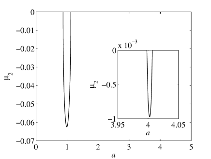
Figure 1: Imaginary part of the critical exponent $\mu$ as function of $a$ for $b=0.25$. Notice the main lobe centered around $a=1$. For the first lobe, the difference between the approximation (13) and the numerics is smaller than the thickness of the line. The second lobe, shown in the inset, is so much smaller than the first one that they can hardly be seen on the same scale.

Investigating $\mu_{2}$ numerically mathematica one finds that (for small positive values of $b$) it consists of a set of symmetrical lobes centered around $a=n^{2}$, where $n$ is a positive integer, the one centered around $a=1$ being substantially larger than the other ones (see Fig. 1). These lobes correspond to the unstable regions. Inspecting these lobes, it is transparent that the most unstable mode corresponds to $a\approx 1$.

One can also argue for the validity of Eq. (12) by analytical means. There is a class of partly-forgotten approximate formulas for $\mu$ as a function of $a$ and $b$ stemming from celestial mechanics (see Ref. critical_exponent for the main results). A convenient formula for our purpose is

$$\mu=\frac{1}{\pi}\arccos\left[\cos\left(\pi\sqrt{a}\right)+\frac{\pi b^{2}\sin\left(\pi\sqrt{a}\right)}{16\sqrt{a}\left(a-1\right)}+\mathcal{O}\left(b^{4}\right)\right],$$ (13)

which describes accurately the first lobe of $\mu_{2}$ for small values of $b$. In order for $\mu$ to have an imaginary part the argument of $\arccos$ must be larger than one (in absolute value). Naturally, identifying the most unstable mode amounts to finding the extremum value of

$$\cos\left(\pi\sqrt{a}\right)+\frac{\pi b^{2}\sin\left(\pi\sqrt{a}\right)}{16\sqrt{a}\left(a-1\right)}.$$

To leading order in $b$ this corresponds to $a=1$.

Finally, numerically solving Eq. (12), one readily obtains $2\pi/k$, which represents the spacing of adjacent maxima, herein called $\cal{S}$, as a function of the driving frequency $\omega$ of the transverse confinement $\omega_{r}$. Neglecting the $k^{4}$ term in Eq. (12), which is numerically small under typical experimental conditions, one has that

$$k = \omega\frac{m^{1/2}}{\omega_{r,0}^{1/2}\hbar^{1/2}}(2a_{s}\rho)^{-1/2}(1+2a_{s}\rho)^{3/4}$$ (14)

$$\times(4+6a_{s}\rho)^{-1/2},$$

where $\rho=N/2L$ is the density of the condensate.

It is important to note that the above formula for $k$ [Eq. (14)] has been obtained by assuming a homogeneous condensate with constant density $\rho=\rho_{0}$. This approximation yields a spacing between adjacent maxima of

$$S_{0}=\frac{2\pi}{k},$$ (15)

where $k$ is computed using Eq. (14) with $\rho=\rho_{0}$. However, the density of the condensate in the considered system is not homogeneous. To account for this inhomogeneity, as a first-order approximation, one uses the fact that, typically for the cases under consideration, the density of the condensate varies on a space scale much larger than that of the observed patterns and thus we can extend Eq. (14) with the density being space dependent: $\rho=\rho(x)$. In fact, the density of the condensate can be approximated in this slowly-varying limit by the so-called Thomas-Fermi (TF) approximation:

$$\rho(x)=3\frac{L^{2}-x^{2}}{4L^{3}},$$ (16)

when $-L<x<L$ and $\rho(x)=0$ otherwise. Therefore, it is possible to approximate the average spacing by taking a spatially averaged $\bar{k}$ for $k$ in Eq. (14) using $\rho(x)$ given by the TF approximation in Eq. (16):

$${\cal S}_{1}=\frac{2\pi}{\bar{k}},$$ (17)

where

$$\bar{k}=\frac{1}{2L}\int_{-L}^{L}k(x)dx.$$ (18)

Alternatively, one could average the spacing directly by using the expression

$${\cal S}_{2}=\frac{1}{2L}\int_{-L}^{L}\frac{2\pi}{k(x)}dx,$$ (19)

where, again, $k(x)$ is given by Eq. (14) with the Thomas-Fermi density $\rho(x)$ of Eq. (16).

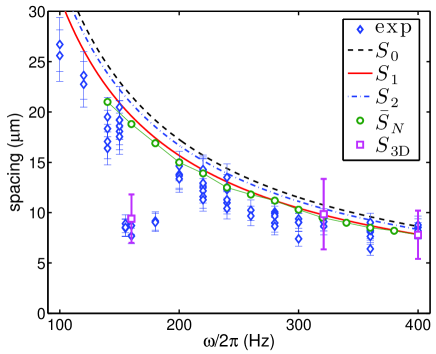
Figure 2: (Color online) Average spacing of adjacent maxima of the longitudinal patterns as a function of the transverse driving frequency. Blue diamond dots depict the experimental data of Ref. engels (the experimental error bar depicted here only takes into account the error bar in the pixel size of the recorded experimental image). Dashed black line, solid red line and blue dashed-dotted line correspond, respectively, to spacings computed using $S_{0}$, $S_{1}$ and $S_{2}$. Green empty circles correspond to spacings extracted from the 1D NPSE numerics by the averaged spacing method. Pink squares correspond to the spacings extracted from the full 3D numerics using the FFT method and its associated error bars (see text for details). Notice that for $\omega/2\pi$ close to 160.5 Hz the theoretical prediction is far from the experimental data. The radial breathing mode excited at these frequencies cannot be captured by the NPSE but is well captured by the 3D numerics.

The above expressions for the spacing $S$ provide the analytical prediction of the present study that can be readily compared quantitatively with the experimental results of Ref. engels . This comparison can be seen in Fig. 2, where the theoretical predictions for $S_{0}$, $S_{1}$ and $S_{2}$ defined above are adapted to the ⁸⁷Rb experiments of Ref. engels , with $\omega_{r,0}/(2\pi)=160.5$ Hz, the condensate length $2L=180~{}\mu$m and $N=5\times 10^{5}$ atoms cond_length . We observe a very good qualitative and a good quantitative agreement between the theoretical predictions and the experimental result, solidifying our expectation that Eq. (14) captures accurately and in a fully analytical way the observed phenomenology of the experiment of Ref. engels . Is it worth mentioning that $S_{1}$ and $S_{2}$ are closer to the experimental data since they account for the inhomogeneity of the cloud. Notice as well that our analytical prediction shows deviations from the experimental data at low frequencies, where the spatial periods of the Faraday waves are comparable with the length of the condensate. At larger frequencies we have good agreement between the theoretical curve and the experimental data, as the periods of the Faraday waves are substantially smaller than the spatial extent of the cloud. The main sources of slight disparity between the theoretical predictions and the experimental results can be traced in the transverse Gaussian (as opposed to Thomas-Fermi) profile and the fact that the analysis cannot directly incorporate the weak longitudinal trapping potential (see the discussion above). These will be further clarified below, through the comparison with the direct numerical simulation results of both the NPSE as well as the full 3D GP equation.

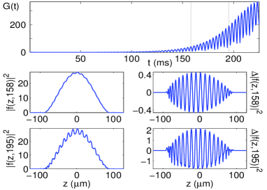
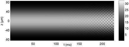
Figure 3: Faraday pattern formation for the 1D NPSE. The top panel depicts the growth rate $G$ ($L^{2}$ norm of the deviation from the initial density) of the pattern. The middle two rows display the Faraday patterns at the times indicated (see vertical lines in top panel) where the left subpanels show the density profile while the right subpanels show the deviation from the initial density profile. The bottom panel depicts the space-time evolution of the density. This case corresponds to the experiment in Ref. engels , namely, a cloud of $N=5\times 10^{5}$ ⁸⁷Rb atoms, trapped by $\{\omega_{r,0},\omega_{z}\}/(2\pi)=\{160.5,7\}$ Hz with a 20% modulation of the radial confinement at a frequency $\omega/(2\pi)=321$ Hz.

III Numerical Results

III.1 One-Dimensional Numerics on the NPSE

Having completed the linear stability analysis, let us now turn to full numerical simulation to investigate the instability onset and the emergence of the relevant Faraday patterns. We have simulated the NPSE (4) for the experimental conditions described in Ref. engels . Specifically, in Fig. 3, we show the formation of the Faraday pattern for a condensed cloud of $N=5\times 10^{5}$ ⁸⁷Rb atoms contained in a magnetic trap with frequencies $\{\omega_{r,0}/(2\pi),\omega_{z}/(2\pi)\}=\{160.5,7\}$ Hz where the radial trap frequency has a modulation of 20% ($\epsilon=0.2$, which is within the typical range of experimentally used modulations) and a frequency $\omega/(2\pi)=321$ Hz corresponding to the resonant oscillation frequency of the radial breathing mode (i.e., $\omega\approx 2\omega_{r,0}$) string1 ; perez2 . As it can be observed from the figure, the Faraday pattern grows exponentially until it is clearly visible in the density space-time evolution (bottom panel) after about 125 ms. It is reassuring that the NPSE is successful in capturing the Faraday pattern with the same wavelength of 10–11 $\mu$m as the experiment of Ref. engels . On the other hand, we have found that the NPSE cannot capture the right time for the development of the instability. The NPSE results take about 125 ms (i.e., about 40 periods of the modulation drive) for the Faraday pattern to be visible while, in the experiments of Ref. engels , some of the patterns are clearly visible after some 10 periods of the drive.

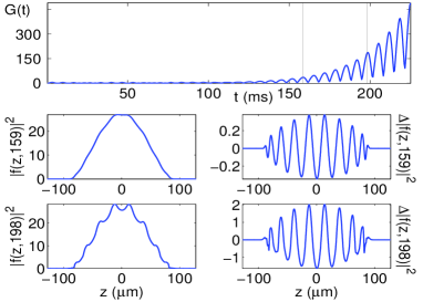
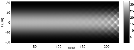
Figure 4: Same as in Fig. 3 for a (stronger) 40% modulation of the radial confinement at a (slower) driving frequency $\omega/(2\pi)=150$ Hz.

A possible explanation for the discrepancy of the Faraday pattern growth between NPSE and the experiments may lie in the size of the initial perturbation, that will eventually seed the Faraday pattern. We have used various amplitudes for the initial perturbation after we obtained the steady state solution to Eq. (4) by imaginary time relaxation. In the results presented in this work we used an initial perturbation with an amplitude randomly chosen in an interval 0.001 times the local density. We also tried larger perturbations, up to ten times larger, and the effect is to accelerate the appearance of the patterns (results not shown here), however we were unable to see distinguishable patterns earlier than 30–35 driving periods for the above setting. Another effect that needs to be taken into account is the amplitude of the modulation drive. While in the experiments of Ref. engels Faraday patterns, for the resonant frequency $\omega/(2\pi)=321$ Hz, quickly formed for even small drive amplitudes (less than 4%, i.e., $\epsilon<0.04$), our numerical results using the NPSE always needed a much larger drive amplitude ($\epsilon=0.2$ in the results of Fig. 3). Therefore, it is clear that the NPSE, although clearly able to capture the nature (wavelength) of the Faraday pattern, it is unable to predict the growth rate of the instability. The reason for this shortcoming stems from the fact that the transverse component of the wavefunction in Eq. (3) is considered to be at its ground state at all times. This is quite a strong assumption considering that the cloud presents impact oscillator-type dynamics for its radial width engels (cf. top panel of Fig. 6 below). This will be verified when we relax the radial wavefunction profile in the 3D simulations shown below.

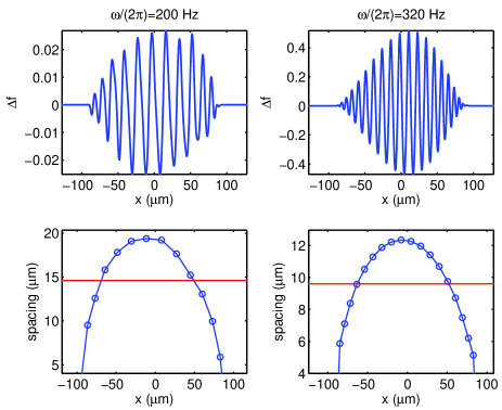
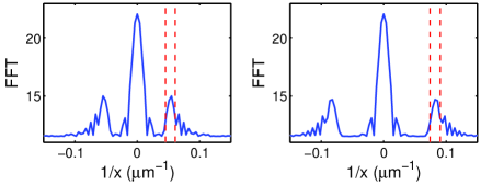
Figure 5: (Color online) Method of averaging spacings in the inhomogeneous cloud for the NPSE model. The left and right columns of plots correspond, respectively, to $\omega/(2\pi)=200$ Hz and $\omega/(2\pi)=320$ Hz. The top row of panels shows the density deviation $\Delta f$ from the initial density profile. The middle row of panels depicts with dots the measured spacing between maxima of $\Delta f$ inside the cloud. The averaged spacing is shown with the red horizontal line. The bottom row of panels shows the FFT of the density $|f|^{2}$. The vertical lines depict the estimated window of the frequencies contained in the Faraday pattern due to the non-homogeneity in the spacings (see middle row).

The results presented in Fig. 3 correspond to the most pattern-forming sensitive case since the drive of the radial frequency is tuned to resonate with the natural breathing frequency of the radial mode. For other driving frequencies, the growth of the Faraday pattern is less pronounced. This is demonstrated in Fig. 4, where we use the same parameter values as in Fig. 3 but changed the driving frequency to $\omega/(2\pi)=150$ Hz and we doubled its amplitude ($\epsilon=0.4$). For this out-of-resonance frequency, the Faraday pattern takes longer to form and even a drive with twice the amplitude takes longer to seed the pattern (the pattern is not visible until approximately 140ms). Nonetheless, it is interesting that this out-of-resonance case only takes about 20 periods to manifest itself.

To summarize the results of the 1D NPSE simulations and to compare them with our analytical prediction for the spacing of the ensuing Faraday patterns, we proceed to measure the averaged spacing in the simulations. The method relies on computing the spacing between maxima on the density deviation $\Delta f$ from the initial profile (see top row in Fig. 5). A couple of examples of the dependence of the spacing inside the cloud are depicted in Fig. 5 together with their average, from now on denoted as $\bar{S}_{N}$. It is clear from these examples that at the center of the cloud, where the density is larger, the spacing is larger than at the periphery of the cloud where the density is lower. The averaged spacing $\bar{S}_{N}$ was computed as a function of the driving frequency and it is depicted by the green empty circles in Fig. 2. As it is clear from Fig. 2, the spacing $S_{1}$ [computed using the analytical expression for the spacing given in Eq. (14) with a spatially averaged density on the TF approximation] and the averaged spacing $\bar{S}_{N}$ from the NPSE dynamics are in good agreement (and the relevant approximation of using Eq. (14) together with Eq. (16) to represent the effects of the longitudinal potential is a fairly accurate one). It is important to mention that the non-homogeneity of the spacings induces an inherent uncertainty in the quantification of the associated spacing for a particular Faraday pattern. The associated window of spacings contained in the Faraday pattern can also be seen from the fast Fourier transform (FFT) spectrum of the density. In the bottom panels of Fig. 5 we depict the FFT spectrum of the density for a couple of cases with their respective frequency windows (see below for further elaboration on this effect).

III.2 Three-Dimensional Numerics

In order to more accurately model the Faraday pattern formation, we used direct numerical simulations of the Gross-Pitaevskii equation (1). The numerics consist of integrating Eq. (1) in cylindrical coordinates. The choice of cylindrical symmetry instead of full 3D numerics is justified by the fact that the radial direction does not develop azimuthal instabilities as it can be observed in the experiments of Ref. engels (and it was also verified by additional tests runs of the full 3D equation on a coarser grid). The main challenge in numerically integrating Eq. (1) stems from the impact oscillator-type dynamics of the radial profile that is driven at resonance. These oscillations produce two numerically challenging effects: (a) they bring most of the atoms close to $r=0$ requiring an extremely fine grid, and (b) as the cloud accelerates during the impact oscillations, the wavefunction oscillates, in space, very rapidly (although the density does not) again requiring a very fine grid. Therefore, although (a) could be circumvented by a grid refinement around $r=0$, challenge (b) requires a fine $r$-grid where the cloud is traveling fastest and this happens on a large portion of the domain. Thus a fine grid needs to be implemented throughout the (radial) $r$-direction, and as a (numerical scheme stability) consequence a very small time step is also required. For the (longitudinal) $z$-direction, it suffices to have enough points to accurately capture the Faraday pattern whose wavelength is quite manageable. In the 3D simulations shown in Figs. 6 and 7 we were able to accurately integrate Eq. (1) for about 7 cycles of the drive with a grid of 2001$\times$401 points in the $(r,z)$-plane with a finite difference scheme in space with 4–5^th Runge Kutta in time with a time step of $0.00025$ (in adimensionalized units).

The initial condition used in the simulations (i.e., the ground state of the condensate) was obtained, as for the 1D case, by imaginary time relaxation.

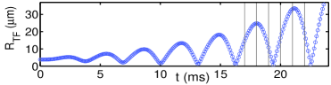
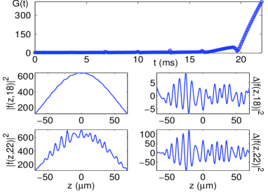
Figure 6: Faraday pattern from the $(r,z)$ 3D simulations. This case corresponds to the experiment in Ref. engels , namely, a cloud of $N=5\times 10^{5}$ ⁸⁷Rb atoms, trapped by $\{\omega_{r,0},\omega_{z}\}/(2\pi)=\{160.5,7\}$ Hz with a 20% modulation of the radial confinement at a driving frequency $\omega/(2\pi)=321$ Hz. The top panel depicts the transverse radius of the cloud displaying impact-oscillator behavior (thin vertical lines depict the times of the snapshots shown in Fig. 7). The second panel depicts the growth of the Faraday pattern while the bottom two rows depict the $r$-integrated density profiles (left subpanels) and their deviation from the initial profile (right subpanels).

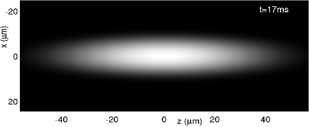
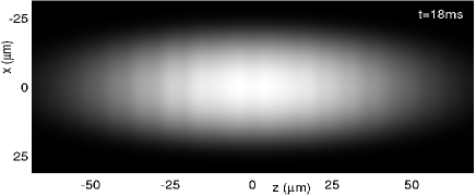
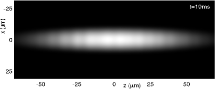
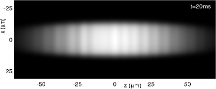
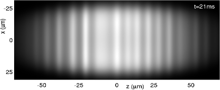
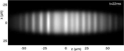
Figure 7: Development of the Faraday pattern in our 3D numerical simulations. Shown are the snapshots of the $y$-integrated profile density (i.e., the observable in the experiments) for the same data as in Fig. 6 at the times indicated.

Figures 6 and 7 depict the Faraday pattern arising from the $(r,z)$ Gross-Pitaevskii simulation for a cloud of $N=5\times 10^{5}$ ⁸⁷Rb atoms driven at resonance ($\omega/(2\pi)=321$ Hz) by a modulation amplitude of 20%, corresponding to the experiments of Ref. engels . Depicted in Fig. 7 is the $y$-integrated (top) view which is what is measured in the experiments. Clearly observable are the well separated fringes of the forming Faraday pattern with an approximate spacing of about 8.5 $\mu$m. Furthermore, in contrast with the NPSE simulations, the Faraday instability develops more rapidly (see second panel in Fig. 6) and it is clearly observable after only 6–7 periods of the drive. As mentioned above, the instability sets in much more rapidly in the full 3D system than in the 1D NPSE reduction, as expected based on the previous discussion. It is worth mentioning that in the 3D simulations we did not introduce a perturbation to the initial condition to seed the Faraday patterns since the inherent numerical noise was capable of starting the pattern.

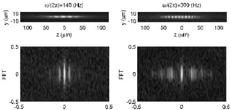
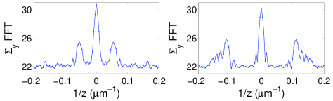
Figure 8: (Color online) FFT analysis for the data from the experiments of Ref. engels . Left and right column correspond, respectively, to a driving frequency of $\omega/(2\pi)=140$ Hz and $\omega/(2\pi)=300$ Hz. The top row depicts the images from the experiment. The second row depicts the corresponding FFTs and the third row the FFTs integrated over the $y$ direction.

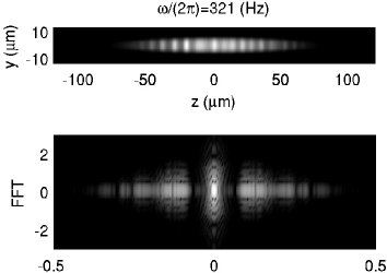
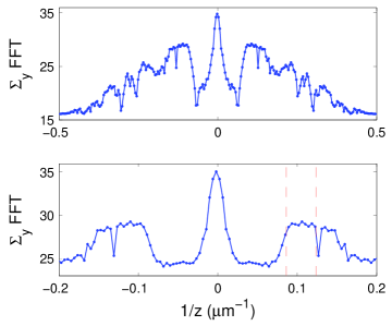
Figure 9: (Color online) FFT analysis from the 3D numerics for $\omega/(2\pi)=321$ Hz. The top two panels depict, respectively, the Faraday pattern and its FFT. The third panel depicts the FFT integrated over the $y$ direction. The bottom panel depicts the same as the third panel but the FFT is computed after adding a 5% noise to the density to simulate the experimental noise in the picture. The vertical lines in the last panel represent our estimated window of possible frequencies for the Faraday pattern (see error bars in the pink square points in Fig. 2).

To validate our full 3D numerics we have computed the average spacing (using the FFT method, see below) for three different cases of the driving frequency. The results are depicted by the pink squares in Fig. 2. As it is evidenced from the figure, the 3D numerical simulations accurately reproduce the spacing from the experiments in Ref. engels including the case when the external driving frequency is half of the resonant frequency (see left-most pink square point in Fig. 2).

In Ref. engels , the sudden drop in the spacing around $\omega/(2\pi)=160$ Hz, i.e., half of the resonant frequency, was attributed to excitation of the radial breathing mode. However, our numerics suggest that this is not the case and that this is due to the fact that we are driving a sub-harmonic that excites the resonance.

It is important to note that the data for the experiment in Ref. engels has a significant variability in the spacing values. This natural experimental variability has many potential sources. Here, we would like to focus on the error generated by the width of the frequency peak used to measure the spacing through the fast Fourier transform (FFT). In the experiments of Ref. engels (see blue diamond dots in Fig. 2), the spacing of the Faraday pattern was measured by computing the FFT of the integrated density image and extracting the spatial frequency of the dominant peak. The error bars depicted in Fig. 2 for the experimental data only take into account the error bar in the pixel size of the experimental snapshots (and not the variability due to the width of the FFT peak, see below).

In Fig. 8 we present a couple of examples (for $\omega/(2\pi)=140$ Hz and $\omega/(2\pi)=300$ Hz) of the Faraday patterns observed in the experiments of Ref. engels . Also in the figure, we depict the FFT of the data (second row) as well as its $y$-integrated counterpart (bottom row). As it is clear from the figure, there is a dominant spatial frequency that can be measured in order to extract the associated spacing of the Faraday pattern. Nonetheless, it is important to note that the dominant peak in the FFT spectrum has a width that indicates an interval of spacings that make up the original Faraday pattern. The width of this peak gives an indication of spatial variability of the pattern spacing: the wider the spectral peak the more spatial variability there exists in the pattern spacing. We have observed the same phenomenology when using our 3D numerical data. A typical example of the FFT analysis of our 3D numerical data is presented in Fig. 9. We have checked that our numerical data is able to reproduce the behavior of the FFT analysis of the experimental data. For a better comparison with experiments we added a 5% random noise to the numerically computed density so as to emulate the noise in the experiment (see bottom panel of Fig. 9). In order to extract the average spacing, $S_{\rm 3D}$, from the 3D numerics we computed the position of the dominant peak in the FFT (see pink square points in Fig. 2). As it is clear from the integrated FFT curves (see bottom two panels in Fig. 9), the Faraday pattern contains a dominant peak with a respective finite width. The width of the peak indicates the presence of a range of spatial frequencies (instead of a single one) and thus we can associate an error bar to the average spacing by taking the width of the dominant peak as the variability in spatial frequencies. This variability has been incorporated in the average spacing of 3D numerical data in Fig. 2 by means of the vertical error bars for the pink square points. In the same spirit, the actual error bar in the experiment should be slightly larger to also account for variability of the spatial frequency due to the width of the computed FFT peaks from the experimental data. Within this variability that, based on Figs. 8 and 9, clearly exists both in the experimental and the numerical (3D) data, we can conclude that our theoretical results are in very good agreement with both their experimental and their numerical counterparts.

IV Conclusions

In this communication, we have revisited the topic of Faraday waves and corresponding resonances in Bose-Einstein condensates. In particular, we have focused on the experimentally relevant case where the transverse confinement is periodically modulated in time. We have used the non-polynomial Schrödinger equation as a tool that permits to present in an explicit form this transverse modulation in an effective longitudinal equation describing the dynamics of the condensate wavefunction. Then, a subsequent modulational stability analysis permitted us to examine the stability of spatially uniform states in this transversely driven, yet effectively one-dimensional setting. This analysis, leading to a Mathieu equation, combined with the well-established theory of the latter equation allowed us to identify the dominant mode of the instability. This, in turn, led us to extract an explicit analytical formula that allows for this mode’s wavenumber (and hence its wavelength which is directly associated with the pattern periodicity and hence is an experimentally observable quantity) as a function of the driving frequency of the transverse confining potential. Direct comparison of the fully analytical result with the experimental observations confirmed the accuracy of our approach. These analytical and experimental results were also corroborated by numerical computations both within the framework of the one-dimensional NPSE equation, as well as for the case of the fully 3D Gross-Pitaevskii equation. The similarities of the two regarding the instability length scale and the differences of the two in connection to the instability growth rate have been accordingly highlighted. These computations have allowed us to validate the quality of our theoretical approximations and give a detailed comparison between theory, numerics and experiment.

There are numerous interesting possibilities that this experiment presents for future studies. One of them is to consider the predominantly two-dimensional case of pancake-shaped condensates, where, depending on the driving frequency, square or rhombic patterns may form. In that setting too, the effective wave equations of Ref. npse may allow to perform the modulational stability analysis and obtain a quantitative handle on the dominant unstable mode. On the other hand, modulations of all three spatial dimensions of the confining potential would be of interest in their own right. In the latter case, while reductions of the type used herein would not be relevant, nevertheless the dynamics may still be analytically describable upon appropriate assumptions, such as, e.g., the quadratic phase assumption of Ref. perez , by means of coupled, nonlinear ordinary differential equations such as Eqs. (12) of Ref. perez . Understanding these settings in more quantitative detail, both analytically, numerically and experimentally, is under current examination and will be reported in future publications.

References

- (1) M.C. Cross and P.C. Hohenberg, Rev. Mod. Phys. 65, 851 (1993).
- (2) M. Faraday, Philos. Trans. R. Soc. London 121, 299 (1831).
- (3) C.J. Pethick and H. Smith, Bose-Einstein condensation in dilute gases, Cambridge University Press (Cambridge, 2002).
- (4) L.P. Pitaevskii and S. Stringari, Bose-Einstein Condensation, Oxford University Press (Oxford, 2003).
- (5) J.J. García-Ripoll, V.M. Pérez-García and P. Torres, Phys. Rev. Lett. 83, 1715 (1999).
- (6) C. Tozzo, M. Krämer, and F. Dalfovo, Phys. Rev. A 72, 023613 (2005).
- (7) M. Krämer, C. Tozzo and F. Dalfovo, Phys. Rev. A 71, 061602(R) (2005)
- (8) C. Schori, T. Stöferle, H. Moritz, M. Köhl, and T. Esslinger Phys. Rev. Lett. 93, 240402 (2005).
- (9) M. Modugno, C. Tozzo, F. Dalfovo, Phys. Rev. A 74, 061601(R) (2006).
- (10) K. Staliunas, S. Longhi and G.J. de Valcárcel, Phys. Rev. Lett. 89, 210406 (2002).
- (11) See e.g. S. Inouye et al., Nature 392, 151 (1998).
- (12) P. Engels, C. Atherton and M.A. Hoefer, Phys. Rev. Lett. 98, 095301 (2007).
- (13) K. Staliunas, S. Longhi and G.J. de Valcárcel, Phys. Rev. A 70, 011601(R) (2004).
- (14) Yu. Kagan and L. A. Manakova, Phys. Lett. A 361, 401 (2007); Yu. Kagan and L. A. Manakova, Phys. Rev. A 76, 023601 (2007).
- (15) M. Fliesser, A. Csordás, P. Szépfalusy and R. Graham, Phys. Rev. A 56, R2533 (1997).
- (16) S. Stringari, Phys. Rev. A 58, 2385 (1998).
- (17) L. Salasnich, A. Parola and L. Reatto, Phys. Rev. A 65, 043614 (2002).
- (18) N. W. McLachlan, Theory and application of Mathieu functions, Oxford University Press, 1951.
- (19) S. Wolfram, The Mathematica book, Wolfram Media/Cambridge University Press, 1999.
- (20) Félix Tisserand, Traité de mécanique céleste, 1894, vol III (see the first chapter on how to derive equation (13)); G. W. Hill, Acta Mathematica VIII, 1886 (reprinted in Collected Mathematical Works, vol I, p. 255); E. L. Ince, Monthly Notices of the Royal Astronomical Society LXXV, 1915, p. 436; J. C. Adams, Collected Scientific Papers, vol I, p. 186, vol II, pp. 65, 86; E. T. Whittaker, Proceedings of the Edinburgh Mathematical Society XXXII, 1914, p. 75.
- (21) The length of the condensate is computed assuming a Thomas-Fermi density profile both radially and longitudinally. For the setup described in Ref. engels one obtains a length of 180 microns, i.e., m.
- (22) S. Stringari, Phys. Rev. Lett. 77, 2360 (1996).
- (23) V. M. Perez-Garcia, H. Michinel, J. I. Cirac, M. Lewenstein, and P. Zoller, Phys. Rev. Lett. 77, 5320 (1996).