Anomalous Diffusion with Absorbing Boundary

Abstract

In a very long Gaussian polymer on time scales shorter that the maximal relaxation time, the mean squared distance travelled by a tagged monomer grows as $\sim t^{1/2}$. We analyze such sub-diffusive behavior in the presence of one or two absorbing boundaries and demonstrate the differences between this process and the sub-diffusion described by the fractional Fokker-Planck equation. In particular, we show that the mean absorption time of diffuser between two absorbing boundaries is finite. Our results restrict the form of the effective dispersion equation that may describe such sub-diffusive processes.

I Introduction

The stochastic fluctuations of a broad range of physical systems fbmgle exhibit a behavior commonly denoted as anomalous diffusion. The random motion is characterized by the scaling of a mean squared coordinate, which (when averaged over many realizations) scales as $t^{\alpha}$ in time $t$. For “normal” diffusion $\alpha=1$, while the cases of $\alpha\neq 1$ are referred to as “anomalous,” with $\alpha<1$, corresponding to sub-diffusion, while $\alpha>1$ describes super-diffusion. The physical origin of anomalous behavior is usually the coupling of the particle (or some other coordinate) to many other degrees of freedom, such that its dynamics is the superposition of numerous other modes with widely distributed time scales. In principle, there is no reason to expect any “universality” in such anomalous processes, and any two situations described by the same exponent $\alpha$ may have very different characteristics. Nevertheless, certain general considerations have motivated approaches that encompass a large variety of cases: for a review see Ref. mkreview .

Many problems related to the behavior of random walkers can be formulated in terms of first passage of a walker, or its absorption at a boundaryfeller ; redner ; weiss . The presence of the absorbing boundary may help to discriminate between different types of anomalous random walkers. Indeed, in the following subsections we shall demonstrate how the study of absorption can be used to gain better understanding of the complexity of anomalous behavior. The behavior of a normal diffuser confined by absorbing boundaries is well understood; in particular, for large times $t$ the survival probability $S(t)$ of such a diffuser decays exponentially. Consequently, the probability density function (PDF) of the diffuser to be absorbed at a particular time $Q(t)=-dS(t)/dt$ also exhibits an exponential decay, leading to a finite mean absorption time. The corresponding result in the case of sub-diffusion is less clear. Only recently it was established fpinf (while building on previously known expressions rd ; mkreview ) that for one-dimensional (1D) sub-diffusion between two absorbing boundaries which is described by a particular (fractional) diffusion equation mkreview , the PDF of absorption $Q(t)$ decays as a small power of $t$, leading to an infinite mean absorption time. The fractional diffusion equation used in this analysis fpinf applies to continuous time random walks, which at each step have a waiting time distribution with a long tail.

A relatively simple and practically important case of sub-diffusion is the motion of a tagged monomer in a long polymer, whose anomalous dynamics was deduced and (numerically) observed by Kremer et al. KBG . A polymer consisting of a large number $N$ of monomers has processes happening on multiple length scales, ranging from the microscopic distance, such as separation between adjacent monomers, $a$, to the size of the polymer. (A measure of the latter is the radius of gyration $R_{g}$. In a good solvent $R_{g}\approx aN^{\nu}$ deGennes_book , with the exponent $\nu\approx 0.59$ in space dimension $d=3$. The “$\approx$” sign indicates omission of a dimensionless prefactor of order unity. In the absence of inter-monomer repulsion $\nu=1/2$ for any $d$.) To these length scales are associated times $\tau_{\rm micro}\approx a^{2}/D_{o}$, below which a selected monomer “does not feel” its surroundings, and $\tau_{N}\approx R_{g}^{2}/D_{\rm CM}\approx a^{2}N^{1+2\nu}/D_{o}$ for how long it takes the polymer to diffuse its own $R_{g}$. Here $D_{o}$ denotes the diffusion constant of a single monomer, while the diffusion constant of the entire polymer, or its center of mass (CM), is $D_{o}/N$. (In this discussion we disregard hydrodynamic interactions.) Very short and very long times correspond to normal diffusion with different diffusion constants. It has been shown in Refs.KBG that for intermediate times $\tau_{\rm micro}<t<\tau_{N}$, the polymer undergoes anomalous diffusion with mean squared distance $\approx a^{2-2\alpha}(D_{o}t)^{\alpha}$, where $\alpha=2\nu/(1+2\nu)$. Note, that sub-diffusion occurs even in the case of the ideal polymer with $\nu=1/2$.

In this work we analyze the sub-diffusive motion of a tagged monomer which is part of an ideal (Gaussian) 1D polymer. While the entire polymer performs diffusive (Monte Carlo) dynamics, we record the position of a single monomer at the mid-point of the chain. In the absence of absorption, this is a simple, analytically solvable problem, and the exact PDF of the monomer position is easily obtained. We could not extend these solutions in the presence of absorbing boundaries, and instead resorted to numerical studies. Indeed, with a single absorbing boundary, the PDF of the monomer position cannot be found using the standard method of images, which is the standard approach for normal diffusion and even some cases of sub-diffusion. We show that when such a particle is placed between two absorbing boundaries, it has a finite mean absorption time, which scales (as expected) with the distance between the absorbing boundaries. Thus, the tagged monomer presents a simple example of sub-diffusion whose survival probability differs drastically from that obtained by application of fractional diffusion.

To provide the basis of comparison with anomalous diffusion, in Sec. II we briefly review the behavior of a normal diffuser in the presence of absorbing boundaries. Our model of the tagged monomer, and the numerical procedure used, are presented in Sec. III. We also present some numerical results confirming the expected sub-diffusive motion of a single monomer. In Secs. IV and V we study the behavior of the tagged monomer in the presence of a single, and a pair of absorbing walls, respectively. We thereby demonstrate the similarities and distinctions between our anomalous diffuser and a normal random walk. Notably, we stress the differences between our case and the solution to the fractional diffusion equation. In the final Sec. VI, we discuss the possible applicability of our results to the the translocation of a polymer through a membrane pore, which was in fact one of the motivations for this study.

II Normal diffusion with absorbing boundaries

The simplest model of a Brownian particle is a random walk (RW) on a discrete lattice, in which both the position of particle $R$ and time (number of steps) $t$ are integers. Exact expressions for the PDF $p(R,t)$, and many other properties, are readily available hughes . A continuum version is the Langevin equation for the motion (diffusion) of a single particle in a solvent (in the high friction limit), moving under the influence of thermal noise kubo :

$$\zeta{\partial R\over\partial t}=\eta(t).$$ (1)

Here $\zeta$ is the friction coefficient, and the thermal noise satisfies $\langle\eta(t)\rangle=0$ (no bias) and $\langle\eta(t)\eta(t^{\prime})\rangle=2\zeta k_{B}T\delta(t-t^{\prime})$. (The angular brackets, $\langle\rangle$, indicate averages over different realizations of the thermal noise.) Starting at $R=0$ at $t=0$, the PDF of particle position at a later time is

$$P(R,t)={1\over\sqrt{2\pi}\sigma}\exp\left(-\frac{R^{2}}{2\sigma^{2}}\right),$$ (2)

where $\sigma^{2}=2D_{o}t$ depends on the diffusion constant $D_{o}=k_{B}T/\zeta$. From the Langevin equation, one can also directly construct the Fokker-Planck (diffusion) equation kubo ; risken for the PDF, as

$${\partial P(R,t)\over\partial t}=D_{o}{\partial^{2}P(R,t)\over\partial R^{2}}.$$ (3)

(Throughout this paper we consider one-dimensional motion; the generalization to higher dimensions is straightforward.)

Consider a diffusing particle starting at the origin and reaching position $R$ at time $t$ without ever touching an absorbing boundary at $R_{\rm a}>0$. The solution of both continuous and discrete versions of this problem have been described in detail by Chandrasekhar chandra . It can be shown that the PDF for the random walker must vanish on the absorbing boundary. Since the diffusion equation is linear, this boundary condition can be satisfied by superposing the PDF of a free particle (Eq. (2)), and one starting at a reflected image as $\tilde{P}(R,t)=P(R,t)-P(R-2R_{\rm a},t)$. The survival probability $S(t)=\int_{-\infty}^{R_{\rm a}}\tilde{P}(R,t)$ reduced by absorption redner , and for large times the absorption PDF decays as $Q(t)\propto t^{-3/2}$. This PDF has diverging mean, since the particle can drift infinitely far in the direction opposite the wall. It should be noted that the image method is specifically suited to random walkers performing independent unit steps; it fails for the sub-diffusive walkers considered in this paper, and also for long-range hops of super-diffusive motion zoia .

If the 1D diffusing particle is confined by two absorbing boundaries, one can still use superposition by the method of images to create a solution. However, in order to satisfy both boundary conditions, an infinite set of images is necessary. A more convenient answer is obtained by expanding the solution in terms of the eigenfunctions of the diffusion equation (3). For a particle enclosed by absorbing boundaries at $R_{\rm a1}=0$ and $R_{\rm a2}=L$, this gives

$$\tilde{P}(R,t)=\sum\limits_{n=1}^{\infty}A_{n}\sin\left({n\pi R\over L}\right)\exp\left[-\left(\frac{n\pi}{L}\right)^{2}D_{o}t\right],$$ (4)

where $\{A_{n}\}$ depend on the initial conditions. Note that at long times $\tilde{P}(R,t)\simeq A_{1}\sin(\pi R/L){\rm e}^{-(\pi/L)^{2}D_{o}t}$, i.e. the PDF has a simple sinusoidal shape with zeroes on the boundaries. The survival probability is $S(t)\propto{\rm e}^{-t/\tau}$, where the characteristic decay time $\tau=L^{2}/\pi^{2}D_{o}$ is of the order of time the particle needs to diffuse over the length of the interval. The PDF for absorption, $Q(t)$, also decays with the same time constant.

Anomalous diffusion can in principle have a myriad of distinct causes. An extensively studied case corresponds to the so-called continuous time random walks for which the waiting time between successive steps is taken from a broad distribution, with power law tails and a diverging mean. The interest in such processes originated in studies of diffusion in semi-conductorspfist , but they eventually became a prototype of anomalous diffusion. The fractional diffusion equation (which involves an integral operator) was developed to describe the evolution of the PDF for such walkers bala ; schneid , and explicit solutions are now available schneid ; hilfer ; metz ; mkreview . Unlike Eq. (2) the solution to these equations is not smooth, but has a cusp at the origin. Another interesting feature is the behavior of the absorption PDF for anomalous diffusers between two absorbing boundaries: it has been shown fpinf , by careful analysis of the solutions rd ; mkreview , that for large times, $Q(t)$ decays as $t^{-(1+\alpha)}$, leading, for $\alpha<1$, to a diverging mean absorption time!

III The model and numerical procedure

A monomer in a polymer undergoes anomalous diffusion even in the trivial case of a phantom chain with no interactions, for which $\nu={1/2}$ in any $d$. For this value of $\nu$, monomer fluctuations are governed by an exponent $\alpha={1/2}$, and thus exhibit sub-diffusion. Since many properties of phantom polymers can be calculated exactly, this presents an excellent model for the study of sub-diffusion. For simplicity, we shall restrict ourselves to the one-dimensional situation; generalization to higher dimensions is straightforward.

After coarse-graining, a sufficiently long flexible polymer can be represented by effective monomers connected to their nearest neighbors by harmonic potentials (Gaussian springs)deGennes_book ; Doi . Thus, the Hamiltonian for a chain of $N$-monomers is

$$H={K\over 2}\sum_{n=1}^{N-1}(R_{n+1}-R_{n})^{2}.$$ (5)

The distribution of the distance between two adjacent (along the chain) monomers at a temperature $T$ is governed by the Boltzmann factor $\exp[-\beta K(R_{n+1}-R_{n})^{2}/2]$, with $\beta=1/(k_{B}T)$ and $k_{B}$ is the Boltzmann constant. The mean squared separation between adjacent monomers is $a^{2}=k_{B}T/K$, while the mean squared radius of gyration is $R_{g}^{2}={1\over 6}N(1-1/N^{2})k_{B}T/K\approx{1\over 6}Nk_{B}T/K$.

Theoretical treatment of the polymer described above requires solution of $N$ coupled Langevin equations. However, the problem becomes particularly simple if we describe the configurations using Rouse modes Doi

$$U_{q}\equiv{1\over N}\sum_{n=1}^{N}R_{n}\cos(q(n-{1\over 2})),$$ (6)

where $q=p\pi/N$, and $p=0,1,\dots N-1$. In terms of $U_{q}$, Langevin equations decouple, and each Rouse mode can be viewed as an independent “particle” moving in a harmonic potential whose strength depends on $q$. The PDF of every $U_{q}$ is Gaussian. Conversely, the position of each monomer can be viewed a linear combination of $U_{q}$s (inverse of Eq. (6)). Since the linear combination of Gaussian variables is a Gaussian variable, we are assured that each monomer is described exactly by a Gaussian PDF, and the theoretical study is reduced to evaluation of the mean and variance of that distribution (see later). In the presence of absorption, such treatment is not possible.

We measured distances in dimensionless units, i.e. multiplied by $\sqrt{K/k_{B}T}$. In these units the the root mean square separation of adjacent monomers is $a=1$, and $R_{g}^{2}\approx N/6$. We used diffusive (Rouse) dynamics to evolve the system in time, i.e. the monomers were moved using standard Monte Carlo (MC) moves. An elementary MC move consists of randomly picking one monomer and attempting to increment its position by $\delta R$ chosen uniformly from the interval (-1,+1), in dimensionless units. The change in the Boltzmann weight factor controls the probabilistic decision of whether the move is accepted. $N$ elementary move attempts are defined as one MC time unit. The mean squared displacement of a monomer in a single move determines the diffusion constant $D_{o}$; with the above choice of step size we had $D_{o}=0.10$.

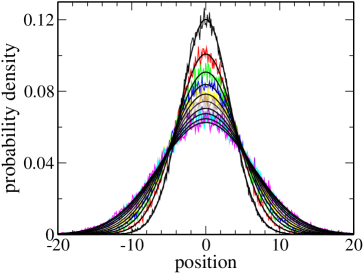
Figure 1: (Color online) PDF for the position of the central monomer in a Gaussian chain of 129 monomers at times $t=2000,4000,\cdots,20000$ (from narrowest to the widest graph). The distributions were obtained from 100,000 runs using bin size $\Delta R=0.1$. The continuous lines represent normalized Gaussian fits to the distributions.

For simulations we chose polymers of odd lengths $N=2^{\ell}+1$, with $\ell=1,2,\cdots,10$, i.e. $N=3,5,9,\cdots,1025$. While all the monomers moved during the simulation, we followed only the position of the central monomer numbered $c=2^{\ell-1}+1$. For each case, 100,000 independent simulations were performed to ensure reliable averages.

As an example, Fig. 1 depicts the PDF of the position of a central monomer ($c=65$) in a Gaussian polymer of $N=129$ monomers. At $t=0$ all monomers were located at the coordinate origin. As the configuration of the polymer evolved in time, the position of the 65th monomer was recorded. Repeating the process 100,000 times produced the distributions shown if Fig. 1. Note the excellent (single parameter) fit of the normalized Gaussian to the actual graphs. Indeed, as explained in the discussion following Eq. (6) the PDF of the monomer must be Gaussian at all times. It should be noted, that this shape is the same as in the case of the normal diffusion, and significantly differs from solutions of sub-diffusive fractional diffusion equations which contain a cusp at the origin (see, Ref. mkreview ).

While the shapes of the graphs in Fig. 1 are not anomalous, the time-dependence of their variance is. For times shorter than the longest relaxation time $\tau_{N}=R_{g}^{2}/2D_{\rm CM}=a^{2}N^{2}/12D_{o}$, which in the above case becomes $\tau_{129}=1.4\times 10^{4}$, the variance of the distribution grows as $t^{1/2}$, while for times longer than $\tau_{N}$ it is linear in $t$. This result can be demonstrated analytically, since the variance of the particle position can be expressed as a sum of variances of Rouse modes. (Analogous calculation for a fluctuating line (or surface) can be found in Ref. kardar_book .) Figure 2 depicts the dependence of the variance on $t$. While all the points are within a half-decade from the crossover point, one can clearly discern the two types of behavior: the slope of the straight line through the first 4 points is 0.52, very close to the expected 1/2, and gradually increases to the right of the graph.

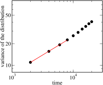
Figure 2: (Color online) Logarithmic plot of the variance of the probability distributions depicted at Fig. 1 as a function of time.

IV A single absorbing boundary

Let us now introduce absorption into the problem. We assume that at $t=0$ all monomers are located at $R=0$, and an absorbing boundary is placed at $R_{\rm a}=8$, i.e. when the central particle reaches this point it is absorbed and the diffusion process ends. It should be stressed that other monomers of the polymer do not feel the absorbing boundary; their sole function is to generate anomalous diffusion of the tagged particle.

We begin with a very short polymer with $N=3$, whose radius of gyration is significantly shorter than $R_{\rm a}$. More importantly, its maximal relaxation time $\tau_{3}\approx 8$ is significantly shorter than the time (about $10^{3}$) for the CM of the polymer to diffuse the distance from the origin to the absorbing boundary. Therefore, at the time-scales at which the particle can be absorbed, the motion of the tagged monomer is indistinguishable from that of the CM of the polymer. Consequently, the problem of absorption of the central monomer should be indistinguishable from that of a normal diffuser with diffusion constant $D_{o}/3$.

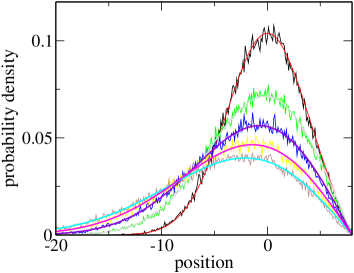
Figure 3: (Color online) PDF of the position of the central particle in a polymer with $N=3$ monomers with an absorbing wall at $R_{\rm a}=8$. The graphs correspond (narrow to broad) to $t=200,400,\cdots 1000$, and solid lines represent fits to the difference of two identical Gaussians centered at $R=0$ and $R=16$. The distributions are obtained from 100,000 runs, and the bin size is $\Delta R=0.1$.

Figure 3 depicts the observed PDF of the position of the central monomer of a polymer with $N=3$ at various times. The area under the graphs decreases with time due to absorption. The shapes are the same as expected for normal single particle diffusion: the solid lines are (single parameter) fits to a difference between two Gaussians centered at image points $R=0$ and $R=2R_{\rm a}$. The excellent fits demonstrate that normal diffusion well describes the absorption for such small $N$. Moreover, the variances of the Gaussians fits increase linearly with time, with a prefactor corresponding to $\sigma^{2}(t)=2D_{\rm CM}t$, in which $D_{\rm CM}$ was calculated independently.

This behavior changes radically when $N$ becomes large. Already for $N=129$ all resemblance to regular diffusion vanishes. The maximal relaxation time $\tau_{129}=1.4\times 10^{4}$ is of the same order as the time required for the CM of the polymer to diffuse the distance to the absorbing boundary (about $4\times 10^{4}$), and $R_{g}$ of the polymer is of the order of the distance to the absorbing boundary. The PDF depicted in Fig. 4 cannot be fitted by the difference between two Gaussians at image points. In particular, the PDF is not linear close to the boundary, but appears to vanish quadratically. Thus the qualitative behavior changes drastically on going from regular diffusion for small $N$ to anomalous diffusion at large $N$.

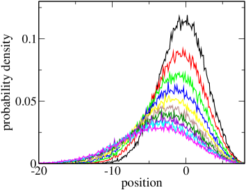
Figure 4: (Color online) PDF of the position of central particle in a polymer with $N=129$ monomers with an absorbing wall at $R_{\rm a}=8$. The graphs correspond (narrow to broad) to times $t=2000,4000,\cdots,20000$. The distributions were obtained from 100,000 runs using bin size $\Delta R=0.1$.

V Two absorbing boundaries

We next consider absorption of the central monomer by two boundaries located at $R_{\rm a}=\pm 8$, for $N$ ranging from 3 to 1025. Figure 5 depicts on a semilogarithmic scale the PDF of the absorption $Q(t)$ for several $N$. For small polymers the curves are indistinguishable from that of a normal random walker with diffusion constant $D_{\rm CM}=D_{o}/N$, which can be calculated from Eq. (4), with $\{A_{n}\}$ selected to correspond to the initial state ($P(R,0)=\delta(R)$). After integrating $\tilde{P}(R,t)$ over $R$ to obtain $S(t)$, we get $Q(t)=-dS/dt$. As explained in Sec. II, for large times $Q(t)$ decays exponentially with a time constant $\tau\approx R_{\rm a}^{2}/D_{\rm CM}=NR_{\rm a}^{2}/D_{o}$. The mean absorption time is of the same order of magnitude. The dependence of the mean time, and of the time constant for decay, is depicted by squares and circles, respectively in Fig. 6. Note that when $N$ becomes large enough, so that the longest relaxation time of the polymer exceeds the typical time it takes for a particle to travel the distance between the absorbing boundaries, $Q(t)$ becomes independent of $N$. Indeed all the graphs for $N=129,257,513,1025$ coincide with each other. The long time behavior remains an exponential decay, as can be seen from the straight lines on the semi-logarithmic plot. These curves thus depict true anomalous diffusion in the “infinite-$N$ limit,” and the corresponding exponential decay time constant scales as the time it takes to cover the interval by sub-diffusion, i.e. $\tau\approx R_{\rm a}^{4}/(a^{2}D_{o})$.

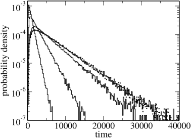
Figure 5: PDF of the absorption time (in Monte Carlo time units) of the central monomer in a Gaussian polymer of length $N$. The tagged monomer can be absorbed at one of two boundaries at $R_{\rm a}=\pm 8$. The plots (from left to right, solid lines) correspond to $N$=3, 9, 33, 129, and $N=513$ (dots), and the histogram was calculated from 100,000 independent runs, with bin size $\Delta t=200$. The graphs for $N=257$, 1025 (not shown), and for $N=129$, are virtually indistinguishable.

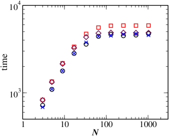
Figure 6: (Color online) The mean first passage (absorption) time (square), and the decay time-constant of the absorption PDF (circle), as a function of polymer size $N$, when all monomers were located at the origin at $t=0$. Diamonds and Xs show the same quantities when at time $t=0$ only the central monomer is at the origin, while the remaining monomers are in a typical equilibrium position. The data are obtained from 100,000 independent runs. The statistical error bars in the mean times (approximately 0.3%), and the estimated systematic errors in the decay time-constants (less than 5%) are much smaller than symbol sizes.

So far, we reported on simulations in which at time $t=0$, the entire polymer is located at the origin, i.e. $R_{n}=0$ for all $n$. This is a particularly convenient choice for analytical calculations, since all Rouse modes vanish at $t=0$ and their mean values (averaged over realizations of the noise) remain zero at all times. In any case, we know that the initial value of each Rouse mode will be forgotten after one relaxation time of that mode. One may consider a different case, where at $t=0$ the polymer assumes a randomly selected equilibrium configuration. Thus, in addition to averaging our results over different realizations, we also need to average over the starting configurations. This initial condition appears more natural since the time $t=0$ is not special. In any case, we find that the differences between the two procedures are rather small. For small $N$ we cannot expect much difference, because by the time the polymer reaches the absorbing boundary it is equilibrated in any case. The results for mean absorption time and decay time constant are depicted by diamonds and Xs, respectively, in Fig. 6. We see that the new procedure gives slightly shorter mean absorption times and essentially the same decay times. Figure 7 depicts the PDF of absorption times for $N=128$. It seems that at short times the random starting point diffuser moves slightly faster leading to shorter mean times, but for large times both cases are characterized by the same decay constant.

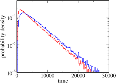
Figure 7: (Color online) PDF of the central monomer of a 129-monomer Gaussian polymer absorbed at boundaries a distance 8 from the initial position on both sides. The curve with the larger mean corresponds to the case when at $t=0$ all $R_{n}=0$, while the other plot corresponds to starting configuration where $R_{c}=0$ while the remaining monomers are equilibrated. This plot (histogram) was calculated from 100,000 independent samples; bin size $\Delta t=200$.

With its exponential decay the long time behavior of a particle between absorbing boundaries more resembles normal diffusion, although the time scales have to be determined using anomalous diffusion arguments. Nevertheless, the PDF of the unabsorbed monomer at long times does not resemble that of a normal diffuser. We studied the PDF of the positions of surviving particles in 100,000 independent runs for a polymer with $N=129$. Naturally, as the time increases the probability of not being absorbed decreases. (The decrease in probability also means that for large $t$ the PDF was derived from samples significantly smaller than 100,000, and consequently the statistical accuracy of the results decreased.) To enable a convenient comparison between the PDFs at various times we normalized them to 1. In the results depicted in Fig. 8, the PDFs of the particle position were recorded at different times, all of the order of mean absorption time. Superficially these results resemble regular diffusion. In analogy to Eq. (4), it appears as if at very long times only a slowest “eigenmode” survives and the PDF decays as $\Psi(R/R_{\rm a}){\rm e}^{-t/\tau}$, with an eigenvalue related to $\tau$. The eigenfunction $\Psi$, depicted in Fig. 8, appears to be universal, although specific to our form of sub-diffusion, while $\tau$ scales as $R_{\rm a}^{4}$ and is independent of $N$.

In the case of a regular diffusion (in the scaled variable $x=R/R_{\rm a}$) we have $\Psi(x)\propto\cos(\pi x/2)$, i.e. the function vanishes at the boundaries ($x=\pm 1$) with a finite slope. By contrast, the results depicted in Fig. 8 suggest a vanishing slope at the boundary. In fact, an attempt to fit the function by a few terms of the Fourier series $b_{0}+b_{1}\cos(\pi x)+\dots$ gives $b_{0}\approx b_{1}$ while the coefficients of higher Fourier components are by an order of magnitude smaller. In Ref. zoia the fractional Laplacian operator was examined in a bounded domain. Their particular implementation of boundary conditions enabled calculation of the eigenfunction $\Psi(x)$ for various values of the fractional order. In particular, the explicit expression for the case corresponding to sub-diffusion with $\alpha=1/2$ in our notation is given in Eq. (A4) of Ref. zoia with $\alpha=4$ in their notation. While this (normalized) function, depicted by a smooth solid line in Fig. 8, qualitatively resembles the numerical curves, it does not provide a quantitative fit. This makes the fractional Laplacian operator a somewhat unlikely candidate for describing the long-time behavior of our diffuser.

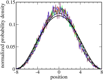
Figure 8: (Color online) Probability density of the position of the central monomer of a 129-monomer polymer, between absorbing walls located at $R_{\rm a}=\pm 8$. The curves are obtained at times $t=2000,4000,6000,8000,10000$, and are the result of 100,000 independent simulations collected in bins of size $\Delta R=0.1$. To remove the effect of absorption all curves have been normalized, such that their integral is unity. The $t=2000$ curve is relatively smooth, while that of $t=10000$ is very noisy because only in a small portion of runs the tagged particle was not absorbed, and consequently the sample size is small. Smooth lines represent two suggested eigenfunctions $\Psi(xR_{\rm a})/R_{\rm a}$: the dashed line corresponds to $\Psi(x)=(1+\cos(\pi x))/2$ (see text), while the solid line represents the normalized eigenfunction given by Eq. (A4) in Ref. zoia .

VI Discussion

In this work we concentrated on an extremely simple, and yet non-trivial model of sub-diffusion. The Gaussian nature allows analytic calculation of some properties, such as the probability distribution of freely moving particles; but the absorption properties were studied numerically. We believe that similar results should apply to self-avoiding polymers, although separation into independent Rouse modes is no longer possible, and probably not much can be done beyond simple scaling arguments. Within our simple model, we find that the process of absorption is quite different from other simplified sub-diffusive processes in the literature.

Anomalous diffusion of a monomer has several features resembling the translocation of a long polymer through a narrow pore in a membrane. This process has been extensively studied experimentally during the last decade kasian ; akeson ; mel . In the theoretical description of translocation, a single variable $s$ representing the monomer number at the pore muthu ; Lubensky ; park ; chern indicates how much of the polymer has passed to the other side. If the translocation process is very slow, the mean force acting on the monomer in the hole can be determined from a simple calculation of entropy, and the translocation problem is reduced to the escape of a ‘particle’ (the translocation coordinate) over a potential barrier. Such theories produce qualitative understanding of experimental results meller_review . However, if the process is not slow enough, compared to the relaxation times of Rouse modes, then its dynamics is more complicated. Successive steps of the reaction coordinate are then correlated in a manner closely resembling the correlations between steps of a tagged monomer in a polymer. In Ref. ckk , it was numerically verified that $s$ indeed undergoes anomalous diffusion in the 1D “space of monomer numbers.” It was further argued that the relaxation of the polymer constrains the translocation process and consequently determines the translocation time. Such behavior closely relates the translocation process to the anomalous diffusion of a single monomer.

In the last few years significant progress has been made in the theoretical modelling of the translocation process. On one hand, short time behavior has been modelled in great detail mathe , and on the other hand scaling consideration of the long time behavior have been extended to include hydrodynamic interactions storm ; tian . Recently Grosberg et al. GrosNech developed an intuitive scaling picture of polymer translocation under the influence of a force. (See also Ref. sakaue .) A variety of scaling regimes with force applied to the end-point or at the pore have been investigated numerically in some detail luo . Some recent studies panja ; dubb suggest that the translocation process maybe even slower than dictated by the relaxation of the Rouse modes. If so, this would weaken the analogy between the translocation and the anomalous diffusion of a monomer. (The accuracy of these claims is questioned in further work luocom .)

To the extent that one may draw an analogy between translocation and anomalous diffusion in the presence of absorbing boundaries, one may inquire whether the mean translocation time is finite. Reference lua argues that translocation may be described by a fractional diffusion equation, and consequently require an infinite mean time, as found in the solutions of such equation fpinf . A similar point is made in Ref. dubb , where a detailed study of the PDF of translocation times is fitted to a slowly decaying function for large times. However, direct (experimental and numerical) measurements appear to indicate well defined average translocation times. Our results offer a model where absorption times of an anomalous diffuser are finite. Clearly more detailed studies of translocation are needed to resolve this question.

In this work we studied in detail the sub-diffusion of a tagged monomer in a Gaussian polymer. In the absence of absorption all properties can be derived analytically. However, upon inclusion of absorbing walls, we had to resort to numerical simulations. While we can characterize all properties of the numerical results, we are still missing an equation that can describe the evolution of the PDF of the position of the tagged particle. In fact, the numerical results exclude several simple forms for such an equation.

- (1) B. B. Mandelbrot and J. W. van Ness, SIAM Rev. 1, 422 (1968); S. C. Lim and S. V. Muniandy, Phys. Rev. E 66, 021114 (2002); E. Lutz, Phys. Rev. E 64, 051106 (2001); A. N. Kolmogorov, Rep. Acad. Sci. USSR 26, 6 (1940); K. G. Wang, L. K. Dong, X. F. Wu, F. W. Zhu, and T. Ko, Physica A 203, 53 (1994); K. G. Wang and M. Tokuyama, Physica A 265, 341 (1999).
- (2) R. Metzler and J. Klafter, Phys. Rep. 339, 1 (2000); and J. Phys. A: Math. Gen. 37, R161 (2004).
- (3) W. Feller, An Introduction to Probability Theory and Its Applications, Wiley, New York (1968).
- (4) S. Redner, A Guide to First-Passage Processes (Cambridge Univ. Press, Cambrdige, 2001).
- (5) G. H. Weiss, Aspects and Applications of the Random Walk (North-Holland, Amsterdam, 1994).
- (6) S. B. Yuste, K. Lindenberg, Phys. Rev. E69, 033101 (2004); M. Gitterman, Phys. Rev. E62, 6065 (2000), and Phys. Rev. E69, 033102 (2004).
- (7) G. Rangarajan and M. Ding, Phys. Rev. E62, 120 (2000).
- (8) K. Kremer and K. Binder, J. Chem. Phys. 81, 6381 (1984); G.S. Grest and K. Kremer, Phys. Rev. A 33, 3628 (1986); I. Carmesin, K. Kremer, Macromolecules 21, 2819 (1988).
- (9) P.-G. de Gennes, Scaling Concepts in Polymer Physics, (Cornell Univ. Press, Ithaca, NY 1979).
- (10) B. D. Hughes, Random Walks and Random Environments, vol. 1 (Clarendon Press, Oxford, 1995).
- (11) R. Kubo, M. Toda and N. Hashitsume, Statistical Physics II, Solid State Sciences, vol. 31 (Berlin, Springer, 1985);
- (12) H. Risken, The Fokker-Planck Equation. Methods of Solution and Applications (Springer, Berlin, 1984).
- (13) S. Chandrasekhar, Rev. Mod. Phys. 15, 1 (1943).
- (14) A. Zoia, A. Rosso, and M. Kardar, Phys. Rev. E 76, 021116 (2007).
- (15) G. Phister and H. Scher, Phys. Rev. B 15, 2062 (1977), and Adv. Phys. 27, 747(1978); H. Scher and E. W. Montroll, Phys. Rev. B 12, 2455 (1975).
- (16) V. Balikrishna, Physica A 132, 569 (1985)
- (17) W. R. Schneider and W. Wyss, J. Math. Phys. 27, 2782 (1982).
- (18) R. Hilfer, Fractals 3, 211 (1995).
- (19) R. Metzler and J. Klafter, Europhys. Lett. 51, 492 (2000).
- (20) M. Doi and S. F. Edwards, The Theory of Polymer Dynamics, Clarendon Press, Oxford (1986).
- (21) M. Kardar, Statistical Physics of Fields, Cambridge University Press, Cambridge (2007), p. 197.
- (22) J. J. Kasianowicz, E. Brandin, D. Branton, and D. W. Deamer, Proc. Natl. Acad. Sci. U.S.A. 93, 13770 (1996).
- (23) M. Akeson, D. Branton, J. J. Kasianowicz, E. Brandin, and D. W. Deamer, Biophys. J. 77, 3227 (1999).
- (24) A. Meller, L. Nivon, E. Brandin, J. Golovchenko, and D. Branton, Proc. Natl. Acad. Sci. U.S.A. 97, 1079 (2000); A. Meller and D. Branton, Electrophoresis 23, 2583 (2002); A. Meller, L. Nivon, and D. Branton, Phys. Rev. Lett. 86, 3435 (2001).
- (25) M. Muthukumar, J. Chem. Phys. 111,10371 (1999).
- (26) D. K. Lubensky and D. R. Nelson, Biophysical Journal 77, 1824 (1999).
- (27) W. Sung and P. J. Park, Phys. Rev. Lett. 77, 783 (1996); P. J. Park and W. Sung, J. Chem. Phys. 108, 3013 (1998).
- (28) Sh.-Sh. Chern, A. E. Cárdenas, R. D. Coalson, J. Chem. Phys. 115, 7772 (2001).
- (29) A. Meller, J. Phys: Cond. Matter. 15, R581 (2003).
- (30) J.Chuang, Y. Kantor, and M. Kardar, Phys. Rev. E65, 011802 (2001); Y. Kantor, and M. Kardar, Phys. Rev. E69, 021806 (2004).
- (31) J. Mathe, A. Aksimentiev, D. R. Nelson, K. Schulten, and A. Meller, Proc. Natl. Acad. Sci. U.S.A. 102, 12377 (2005). A. Aksimentiev, J. B. Heng, G. Timp nad K. Schulten, Biophys. Journal 87, 2086 (2004).
- (32) A. J. Storm, C. Storm, J. Chen, H. Zandbergen, J. F. Joanny, and C. Dekker, Nano Lett. 5, 1193 (2005).
- (33) P. Tian and G. D. Smith, J. Chem. Phys. 119, 11475 (2003).
- (34) A. Yu. Grosberg, S. Nechaev, M. Tamm, O. Vasilyev, Phys. Rev. Lett. 96, 228105 (2006).
- (35) T. Sakaue, Phys. Rev. E 76, 021803 (2007).
- (36) K. Luo, I. Huopaniemi, T. Ala-Nissila, S.-Ch. Ying, J. Chem. Phys. 124, 114704 (2006); K. Luo, T. Ala-Nissila, S.-Ch. Ying, J. Chem. Phys. 124, 034714 (2006); I. Huopaniemi, K. Luo, T. Ala-Nissila, S.-Ch. Ying, J. Chem. Phys. 125 124901 (2006); I. Huopaniemi, K. Luo, T. Ala-Nissila, S.-Ch. Ying, Phys. Rev. E. 75, 061912 (2007).
- (37) J. Klein Wolterink, G. T. Barkema, and D. Panja, Phys. Rev. Lett. 96, 208301 (2006); D. Panja, G. T. Barkema and R. C. Ball, arXiv:cond-mat/0610671 and arXiv:cond-mat/0703404.
- (38) J. L. A. Dubbeldam, A. Milchev, V. G. Rostiashvili, and T. A. Vilgis, Phys. Rev. E 76, 010801 (R) (2007).
- (39) K. Luo, T. Ala-Nissila, S.-Ch. Ying, P. Pomorski and M. Kattunen, arXiv:0709.4615.
- (40) R. C. Lua, A. Y. Grosberg, Phys. Rev. E 72, 61918 (2005).