Tangles of superpositions and the convex-roof extension

Abstract

We discuss aspects of the convex-roof extension of multipartite entanglement measures, that is, $SL(2,{\rm\kern 2.40005pt\vrule width=0.39993pt,height=6.28612pt,depth=-0.3014pt\kern-3.00003ptC})$ invariant tangles. We highlight two key concepts that contain valuable information about the tangle of a density matrix: the zero-polytope is a convex set of density matrices with vanishing tangle whereas the convex characteristic curve readily provides a non-trivial lower bound for the convex roof and serves as a tool for constructing the convex roof outside the zero-polytope. Both concepts are derived from the tangle for superpositions of the eigenstates of the density matrix. We illustrate their application by considering examples of density matrices for two-qubit and three-qubit states of rank 2, thereby pointing out both the power and the limitations of the concepts.

I Introduction

One of the challenges in present quantum information theory is the quantification of multipartite entanglement both in pure and mixed states Plenio and Virmani (2007). Once a measure for pure multipartite states is given (a “tangle” – that is, a polynomial invariant, see below), the corresponding measure for mixed states can be obtained via the convex-roof extension Uhlmann (1998). Although its definition is straightforward, the practical evaluation of the convex-roof extension is a difficult mathematical problem. To date a general analytical method is known only for the concurrence of two-qubit mixed states Wootters (1998); Uhlmann (2000).

The convex roof is obtained by minimizing the average tangle of a given mixed state over all possible decompositions of that state into pure states. As all elements in a decomposition are superpositions of the eigenstates of the given density matrix, the minimal tangle will depend on the possible tangle values for those superpositions.

Recently, several authors have discussed how the entanglement of superpositions of some given pure states is related to the entanglement contained in those states Linden et al. (2006); Cavalcanti et al. (2007); Gour (2007); Niset and Cerf (2007); Song et al. (2007). Here, we are considering a different problem, namely how the entanglement of a mixed state depends on the entanglement of the superposition of its constituents. To this end, we introduce two concepts that facilitate the evaluation of mixed-state tangles for rank-2 states: the zero polytope and the convex characteristic curve. For a given mixed state $\rho$, the zero polytope is the convex set of those density matrices which have eigenstates in the range of $\rho$ and, at the same time, have vanishing tangle. On the other hand, the convex characteristic curve is the largest convex function (of a suitable parameter) that does not exceed the tangle of any pure state in the range of $\rho$ (for detailed explanation see below).

The outline of this article is as follows. First, we introduce some terminology (Section II) and then give precise definitions of the zero polytope and the characteristic curve (Section III). There, we also discuss implications for the convex roof of the tangle in rank-2 states as well as the possible extension of these concepts to ranks larger than two. In Section IV we illustrate the application to examples of rank-2 states of two and three qubits.

II Basic concepts

II.1 Pure-state entanglement measures

A function quantifying entanglement is required to be an entanglement monotone Vidal (2000). Its crucial property is that it be non-increasing (on average) under stochastic local operations and classical communication (SLOCC). Stochastic local equivalence of two $N$-qubit states is represented by convertibility under $SL(2,{\rm\kern 2.40005pt\vrule width=0.39993pt,height=6.28612pt,depth=-0.3014pt\kern-3.00003ptC})^{\otimes N}$ transformations Bennett et al. (2000); Dür et al. (2000), and a homogeneous function on $N$ qubits that is invariant under such operations is an entanglement monotone Verstraete et al. (2003).

Here we investigate entanglement measures related to the concurrence introduced by Wootters and co-workers Hill and Wootters (1997); Wootters (1998); Coffman et al. (2000).

The concurrence $C(\phi_{AB})$ measures the degree of bipartite entanglement shared between the parties $A$ and $B$ in a pure two-qubit state $\left|\phi_{AB}\right\rangle\in{\cal H}_{A}\otimes{\cal H}_{B}$. In terms of the coefficients $\{\phi_{00},\phi_{01},\phi_{10},\phi_{11}\}$ of $\left|\phi_{AB}\right\rangle$ with respect to an orthonormal basis of product states it is defined as

$$C(\phi_{AB})\ =\ 2|\phi_{00}\phi_{11}-\phi_{01}\phi_{10}|\ \ .$$ (1)

The concurrence is maximal for Bell states such as $(\left|00\right\rangle+\left|11\right\rangle)/\sqrt{2}$ while it vanishes for factorized states.

A measure for three-party entanglement has been introduced in Ref. Coffman et al. (2000). The 3-tangle $\tau_{3}(\psi)$ of a three-qubit state $\psi\in{\cal H}_{A}\otimes{\cal H}_{B}\otimes{\cal H}_{C}$ can be expressed by using the wavefunction coefficients $\{\psi_{000},\psi_{001},\ldots,\psi_{111}\}$ as

$$\tau_{3} = 4\ |d_{1}-2d_{2}+4d_{3}|$$

$$d_{1} = \psi^{2}_{000}\psi^{2}_{111}+\psi^{2}_{001}\psi^{2}_{110}+\psi^{2}_{010}\psi^{2}_{101}+\psi^{2}_{100}\psi^{2}_{011}$$

$$d_{2} = \psi_{000}\psi_{111}\psi_{011}\psi_{100}+\psi_{000}\psi_{111}\psi_{101}\psi_{010}$$

$$+\psi_{000}\psi_{111}\psi_{110}\psi_{001}+\psi_{011}\psi_{100}\psi_{101}\psi_{010}$$

$$+\psi_{011}\psi_{100}\psi_{110}\psi_{001}+\psi_{101}\psi_{010}\psi_{110}\psi_{001}$$

$$d_{3} = \psi_{000}\psi_{110}\psi_{101}\psi_{011}+\psi_{111}\psi_{001}\psi_{010}\psi_{100}\ \ .$$

For the GHZ state

$$\left|GHZ\right\rangle\ =\ \frac{1}{\sqrt{2}}\ (\left|000\right\rangle\ +\ \left|111\right\rangle)$$ (2)

the 3-tangle becomes maximal: $\tau_{3}(GHZ)=1$, and it vanishes for any factorized state. It is most remarkable that there is a class of entangled three-qubit states for which $\tau_{3}$ vanishes, i.e., these states are not SLOCC equivalent to any GHZ-type state Dür et al. (2000). This class is represented by the $\left|W\right\rangle$ state

$$\left|W\right\rangle\ =\ \frac{1}{\sqrt{3}}\ (\left|100\right\rangle\ +\ \left|010\right\rangle\ +\ \left|001\right\rangle)\ \ ,$$ (3)

and it is easy to check that $\tau_{3}(W)=0$.

Both concurrence and the 3-tangle are the unique two- and three-qubit versions of more general polynomial measures invariant under local $SL(2,{\rm\kern 2.40005pt\vrule width=0.39993pt,height=6.28612pt,depth=-0.3014pt\kern-3.00003ptC})$ transformations Verstraete et al. (2003); Leifer et al. (2004). These quantities are homogeneous of even degree in the coefficients of the wavefunction (with respect to a product basis) and play an important role as fundamental $SL(2,{\rm\kern 2.40005pt\vrule width=0.39993pt,height=6.28612pt,depth=-0.3014pt\kern-3.00003ptC})$ invariants in invariant theory Briand et al. (2003). Therefore they serve as class-selective measures of (multipartite) entanglement Osterloh and Siewert (2005, 2006). In what follows, we refer to such polynomial invariants as tangles.

II.2 Entanglement measures for mixed states – convex-roof extension

Given a continuous real function $g$ on the space of pure states $\Omega^{\mathbf{ex}}$, this function can be extended to the space of mixed states in the following way Bennett et al. (1996); Benatti et al. (1996); Uhlmann (2000). Let $\Omega$ be the convex (and compact) set of normalized density operators. A state $\rho\in\Omega$ can be written as a convex combination

$$\rho\ =\ \sum_{j}p_{j}\pi_{j},\ \ \ \ \ \pi_{j}:=\frac{\left|j\right\rangle\!\left\langle j\right|}{\langle j|j\rangle}$$ (4)

where the pure states $\pi\in\Omega^{\mathrm{ex}}$ are extremal points of $\Omega$. The real function $g^{\cup}:\Omega\to\mathbb{R}$ is a convex-roof extension of $g:\Omega^{\mathrm{ex}}\to\mathbb{R}$ if $g^{\cup}$ coincides with $g$ on $\Omega^{\mathrm{ex}}$ and

$$g^{\cup}(\rho)\ :=\ \min\sum p_{j}g(\pi_{j})\ \ .$$ (5)

where the minimum is taken over all decomposition of $\rho$. With this in mind it is formally straightforward to extend the definition of the concurrence to mixed two-qubit states $\rho$ with a decomposition $\rho=\sum p_{j}\pi_{j}^{AB}$ into pure two-qubit states $\pi_{j}^{AB}$ of the parties $A$ and $B$

$$C(\rho)\ =\ \min\sum p_{j}C(\pi_{j}^{AB})\ \ .$$ (6)

Correspondingly, we have the 3-tangle for mixed three-qubit states $\rho=\sum p_{j}\pi_{j}^{ABC}$

$$\tau_{3}(\rho)\ =\ \min\sum p_{j}\tau_{3}(\pi_{j}^{ABC})$$ (7)

where $\pi_{j}^{ABC}$ denote pure three-qubit states. A decomposition for which the minimum of the respective function is realized, is called an optimal decomposition.

III Entanglement of superpositions and implications for the convex roof

It is in general difficult to evaluate the convex-roof extension, i.e. the tangle of a given density matrix $\rho$. To this end, it is required to study the entanglement of pure states in the range of $\rho$, ${\cal R}_{\rho}$, as can be seen from Definition (5). Our starting point is the observation that the pure states $\left|\psi\right\rangle_{\rho}\in{\cal R}_{\rho}$ are superpositions of the eigenstates of $\rho$.

III.1 Density matrices with vanishing tangle: the zero-polytope

An important question is whether or not a tangle $\tau$ vanishes for a given $\rho$. That is, we ask whether there is a decomposition of $\rho$ into pure states $\{\left|\psi_{j}\right\rangle_{\rho}\}$ such that $\tau(\left|\psi_{j}\right\rangle_{\rho})=0$ for all $j=0,\ldots,r^{2}-1$ where $r$ is the rank of $\rho$. A polynomial $SL(2,{\rm\kern 2.40005pt\vrule width=0.39993pt,height=6.28612pt,depth=-0.3014pt\kern-3.00003ptC})$ invariant $\tau$ is a homogeneous function of the coefficients of $\left|\psi\right\rangle_{\rho}$. The homogeneous degree of $\tau$ (denoted by $h$) is an even positive integer. Writing $\left|\psi\right\rangle_{\rho}=\sum_{j=0}^{r-1}z_{j}\left|\psi_{j}\right\rangle$, this implies that $\tau(\left|\psi\right\rangle_{\rho})$ is a polynomial of degree $h$ in the complex variables $z_{0},\dots,z_{r-1}$. The situation is most easily understood by considering rank-2 density matrices. Let us assume there is at least one eigenstate $\left|\psi_{1}\right\rangle$ of $\rho$ such that $\tau(\psi_{1})\neq 0$ (otherwise we have trivially $\tau(\rho)=0$). Since normalization does not play any role for this question, we then write

$$\left|\psi\right\rangle_{\rho}=\left|\psi_{0}\right\rangle+z\left|\psi_{1}\right\rangle\ \ .$$ (8)

The tangle is then a polynomial of degree $h$ of a single complex variable $z$ and consequently has precisely $h$ zeros $\zeta_{1},\dots,\zeta_{h}$. If both states have zero tangle we have to add the solution $z=\infty$ to the $h-1$ finite solutions of $\tau(\left|\psi\right\rangle_{\rho})=0$. These zeros correspond to $h$ pure states

$$\left|Z_{1}\right\rangle_{\rho} = \left|\psi_{0}\right\rangle+\zeta_{1}\left|\psi_{1}\right\rangle$$

$$\vdots$$

$$\left|Z_{h}\right\rangle_{\rho} = \left|\psi_{0}\right\rangle+\zeta_{h}\left|\psi_{1}\right\rangle$$

satisfying $\tau(Z_{j})=0$ for all $j=1,\dots,h$. They span a polytope with $h$ corners that contains precisely those density matrices which can be decomposed into these states, i.e., all convex combinations of $\pi_{{}_{Z_{1}}},\dots,\pi_{{}_{Z_{h}}}$. All the density matrices in this polytope have zero tangle (and outside there is no other state with zero tangle) and therefore we call it the zero-polytope; its occurrence is generic for all polynomial $SL(2,{\rm\kern 2.40005pt\vrule width=0.39993pt,height=6.28612pt,depth=-0.3014pt\kern-3.00003ptC})$-invariant entanglement monotones. This includes the concurrence, 3-tangle and multipartite entanglement monotones constructed in Osterloh and Siewert (2005, 2006).

We will now discuss briefly how the concept of the zero-polytope can be extended to higher-rank density matrices. As the tangle of homogeneous degree $h$ evaluated on the pure state gives a polynomial of degree $h$ in the variables $z_{j}$, for $z_{2},\dots,z_{r-1}$ kept fixed, we return to the situation explained above, and the remaining polynomial has precisely $h$ zeros, $\zeta_{j}(z_{2},\dots,z_{r-1})$ with corresponding states

$$\left|Z_{j};z_{2},\dots,z_{r-1}\right\rangle=\left|\psi_{0}\right\rangle+\zeta_{j}(z_{2},\dots,z_{r-1})\left|\psi_{1}\right\rangle+\sum_{k=2}^{r-1}z_{j}\left|\psi_{j}\right\rangle\ .$$

Upon varying $z_{2},\dots,z_{r-1}$, each of these states will describe an $2(r-2)$ dimensional (real) manifold in the $r^{2}-2$ dimensional manifold of states $\left|\psi\right\rangle\left\langle\psi\right|$. The convex hull of the union of these $h$ manifolds contains exactly all density matrices in ${\cal R}_{\rho}$ with zero tangle.
Below we will discuss the zero-polytope for two explicit examples with rank $r=2$.

III.2 The convex characteristic curve

It is well-known Schrödinger (1936) that from the decomposition of a rank-$r$ density matrix $\rho=\sum_{j=0}^{r-1}p_{j}\left|\psi_{j}\right\rangle\!\left\langle\psi_{j}\right|$ into its eigenstates $\{\left|\psi_{j}\right\rangle\}$, any other decomposition $\rho=\sum_{l}\left|\chi_{l}\right\rangle\!\left\langle\chi_{l}\right|$ of length $m\geq r$ can be obtained with a unitary $m\times m$ matrix $U_{lj}$ via $\left|\chi_{l}\right\rangle\ =\ \sum_{j=0}^{m-1}U_{lj}\sqrt{p_{j}}\left|\psi_{j}\right\rangle$. Therefore, the tangle of all pure states $\left|\psi\right\rangle_{\rho}$

$$\left|\psi\right\rangle_{\rho}\ =\ \sum_{j=0}^{r-1}c_{j}\left|\psi_{j}\right\rangle\ \ ,\ \ \ \ \ \sum_{j}|c_{j}|^{2}=1$$

can be regarded as a finger print of the tangle for all density matrices in ${\cal R}_{\rho}$. This suggests to look for the minimum tangle of states $\left|\psi\right\rangle_{\rho}$; but rather than taking the global minimum, which is zero, we will look for local minima when the weights in the superposition are kept fixed. The degrees of freedom for this minimization are the relative phases in the superposition. In an appropriate geometric representation, these minima describe characteristic curves of the tangle as a function of the weights.

Let us discuss the simplest case first, that is, a rank-2 density matrix with its eigendecomposition

$$\rho=p_{0}\left|\psi_{0}\right\rangle\!\left\langle\psi_{0}\right|+p_{1}\left|\psi_{1}\right\rangle\!\left\langle\psi_{1}\right|$$ (9)

with $p_{j}\in{\rm\vrule width=0.39993pt,height=6.80275pt,depth=0.0pt\kern-0.39993ptR}$, $0\leq p_{j}\leq 1$ such that $p_{0}+p_{1}=1$.

All pure states in ${\cal R}_{\rho}$ can be written as

$$\left|\psi\right\rangle_{\rho}=\sqrt{q}\left|\psi_{0}\right\rangle+\sqrt{1-q}{\rm e}^{i\varphi}\left|\psi_{1}\right\rangle$$ (10)

where $q,\varphi\in{\rm\vrule width=0.39993pt,height=6.80275pt,depth=0.0pt\kern-0.39993ptR}$ and $0\leq q\leq 1$, $0\leq\varphi\leq 2\pi$. We may consider the tangle $\tau$ of such a state (for a given phase $\varphi$) as a function of $q$ in a $\tau-q$ diagram (cf. also Fig. 1). This function represents a “characteristic curve” for $\tau$ and is in general not convex.

Clearly, each point $(q,\tau(\psi(q,\varphi)))$ in the $\tau-q$ plane stands for the tangle of the pure state projector $\left|\psi(q,\varphi)\right\rangle_{\rho}\!\left\langle\psi(q,\varphi)\right|$. Now consider an alternative length-2 decomposition of $\rho$, $\rho=\tilde{p}_{0}\left|\phi_{0}\right\rangle_{\rho}\!\left\langle\phi_{0}\right|+\tilde{p}_{1}\left|\phi_{1}\right\rangle_{\rho}\!\left\langle\phi_{1}\right|$.

The states $\left|\phi_{0}\right\rangle_{\rho}$ and $\left|\phi_{1}\right\rangle_{\rho}$ have the we weights $q_{0}$, $q_{1}$ and the relative phases $\varphi_{0}$ and $\varphi_{1}$. As these states form a decomposition of $\rho$ their parameters obey $p_{0}=\tilde{p}_{0}q_{0}+\tilde{p}_{1}q_{1}$. Moreover, the phases need to be adjusted properly. Note that, for arbitrary phases, a density matrix $p_{0}\left|\psi_{0}\right\rangle_{\rho}\!\left\langle\psi_{0}\right|+p_{1}\left|\psi_{1}\right\rangle_{\rho}\!\left\langle\psi_{1}\right|+\alpha\left|\psi_{0}\right\rangle_{\rho}\!\left\langle\psi_{1}\right|+{\rm h.c.}$ is obtained which, in the eigenbasis, has the correct diagonal elements.

The average tangle of the decomposition $\rho=\tilde{p}_{0}\left|\phi_{0}\right\rangle_{\rho}\!\left\langle\phi_{0}\right|+\tilde{p}_{1}\left|\phi_{1}\right\rangle_{\rho}\!\left\langle\phi_{1}\right|$ is visualized in the $\tau-q$ plane by connecting the points $(q_{0},\tau(q_{0},\varphi_{0}))$ and $(q_{1},\tau(q_{1},\varphi_{1}))$ corresponding to the tangle of the states $\left|\phi_{0}\right\rangle_{\rho}$, $\left|\phi_{1}\right\rangle_{\rho}$ by a straight line.

Its value $\tilde{p}_{0}\tau(\phi_{0})+\tilde{p}_{1}\tau(\phi_{1})$ is assumed for the abscissa value $q\equiv p_{0}=\tilde{p}_{0}q_{0}+\tilde{p}_{1}q_{1}$. The generalization to decompositions of $\rho$ of length $>2$ is straightforward. Hence, a given decomposition of $\rho$ can be assigned a point in the $\tau-q$ plane with abscissa $p_{0}$ and ordinate equal to the average tangle $\tau$ that results from convexly combining the tangles of the

pure states in the decomposition.

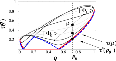
Figure 1: Characteristic curves $\tau(q,\varphi)$ in the $\tau-q$ plane (solid gray lines) for the superpositions in Eq. (10). The (blue) dashed line represents the minimum $\tilde{\tau}(q)$ from Eq. (11) and the solid (red) line its function convex hull $\tau^{\ast}(q)$, i.e., the convex characteristic curve (for details see text).
The point with label $\rho$ indicates the average tangle of a particular length-2 decomposition of the density matrix $\rho=\tilde{p}_{0}\left|\phi_{0}\right\rangle+\tilde{p}_{1}\left|\phi_{1}\right\rangle$. Moreover we illustrate the actual tangle of this density matrix $\tau(\rho)$ and its lower bound $\tau^{\ast}(p_{0})$ according to the convex characteristic curve.

The actual value of the tangle $\tau(\rho)$ is the minimum for all possible decompositions. In our geometric visualization this means to find the smallest possible $\tau(p_{0})$ that may result from a convex combination of at most $r^{2}$ pure states. In order to find this value of $\tau$ (or at least approximate it) one may try the following approach: first minimize the pure-state tangle $\tau(q,\varphi)$ for each argument $q$

$$\tilde{\tau}(q)\ =\ \min_{\varphi}{[\tau(\psi(q,\varphi))]}$$ (11)

and then try to find decompositions from these minimal values $\tilde{\tau}(q)$. That is, we need to investigate convex combinations of pure states and their corresponding tangle. However, we note that the function $\tilde{\tau}(q)$ is in general not convex.

Therefore we define $\tau^{\ast}(q)$ as the function convex hull of $\tilde{\tau}(q)$ (i.e., the largest convex function that does not exceed $\tau(q,\varphi)$) and call it the convex characteristic curve. It is not difficult to see that the convex characteristic curve provides a non-trivial lower bound for the tangle $\tau(\rho)$ of the initial rank-2 density matrix $\rho$. Any (normalized) vector $\left|\phi_{j}^{\mathrm{opt}}\right\rangle_{\rho}$ in an optimal decomposition of $\rho=\sum p_{j}^{\mathrm{opt}}\left|\phi_{j}^{\mathrm{opt}}\right\rangle_{\rho}\!\left\langle\phi_{j}^{\mathrm{opt}}\right|$ is characterized by some $q_{j}$ and a phase $\varphi_{j}$ in analogy with Eq. (10). A lower bound for the tangle of the pure state $\left|\phi_{j}^{\mathrm{opt}}\right\rangle_{\rho}\!\left\langle\phi_{j}^{\mathrm{opt}}\right|$ is given by the convex characteristic curve: $\tau(\phi_{j}^{\mathrm{opt}})\geq\tau^{\ast}(q_{j})$. Consequently, the tangle of $\rho$ is bounded from below by the convex combination $\sum p^{\mathrm{opt}}_{j}\tau^{\ast}(q_{j})$ of the points $\{(q_{j},\tau^{\ast}(q_{j}))\}$ on the convex characteristic curve. As the weight of $\left|\psi_{0}\right\rangle$ in $\rho$ equals $p_{0}$ we find

$$\tau(\rho)=\sum p_{j}^{\mathrm{opt}}\tau(\phi_{j}^{\mathrm{opt}})\geq\sum p_{j}^{\mathrm{opt}}\tau^{\ast}(q_{j})\geq\tau^{\ast}(p_{0})\ .$$ (12)

This is a tight estimate of $\tau(\rho)$. The equal sign in the first inequality in Eq. (12) holds if and only if there is an optimal decomposition such that all points corresponding to the states of this decomposition lie on the convex characteristic curve. For the equal sign in the second inequality in Eq. (12), either $\tau^{*}$ must be affine or all $q_{i}$ have to coincide.

If the rank of the given density matrix is larger than two, the convex characteristic curve can be generalized to a convex manifold. Suppose we have a family of rank-$r$ density matrices with its eigendecomposition

$$\rho\ =\ p_{0}\left|\psi_{0}\right\rangle\!\left\langle\psi_{0}\right|+\ldots+p_{r-1}\left|\psi_{r-1}\right\rangle\!\left\langle\psi_{r-1}\right|$$ (13)

and $\sum_{j=0}^{r-1}p_{j}=1$. Then we define

$$\tilde{\tau}(q_{0},\dots,q_{r-2}) = \min_{\vec{\varphi}}\tau[\psi(q_{0},\dots,q_{r-2};\varphi_{1},\dots,\varphi_{r-1})]$$ (14)

$$\left|\psi(q_{0},\dots,q_{r-2};\varphi_{1},\dots,\varphi_{r-1})\right\rangle = \sqrt{q_{0}}\;\left|\psi_{0}\right\rangle+\sum_{j=1}^{r-1}\sqrt{q_{j}}\;{\rm e}^{i\varphi_{j}}\left|\psi_{j}\right\rangle$$ (15)

with $q_{j}\in{\rm\vrule width=0.39993pt,height=6.80275pt,depth=0.0pt\kern-0.39993ptR}$ such that $\sum_{j=0}^{r-1}q_{j}=1$. The convex characteristic manifold $\tau^{\ast}(q_{0},\ldots,q_{r-2})$ is then defined as the function convex hull of $\tilde{\tau}(q_{0},\ldots,q_{r-2})$.

In analogy with the rank-2 case, the value of $\tau^{\ast}(p_{0},\ldots,p_{r-2})$ gives a strict lower bound for the tangle of the density matrix in Eq. (13). However, due to its higher dimensionality it is much more difficult than in the rank-2 case to completely characterize this manifold and use it for estimates. Even as a tool for a numerical or graphical method it will be rather hard to handle.

In order to illustrate the relevance of the convex characteristic curves/manifolds, but to also highlight caveats, we discuss two examples on specific rank-2 density matrices for two and three qubits.

IV Examples

In the following we illustrate the concepts introduced above in two examples: three-qubit mixtures of GHZ and W states Lohmayer et al. (2006), and a generic two-qubit example. While in the highly symmetric three-qubit case the convex characteristic curve leads directly to an analytic solution for the convex roof of a whole family of states, the two-qubit example shows that in general the convex characteristic curve will give a lower bound for the mixed-state tangle but not necessarily a tight one.

IV.1 Mixed three-qubit states with GHZ and W components

For three qubits, the GHZ state and the W state are given by Eqs. (2) and (3), respectively. We note that the 3-tangle of the GHZ state is maximal: $\tau_{3}(GHZ)=1$ while it vanishes for the W state $\tau_{3}(W)=0$ Coffman et al. (2000). Moreover, we have $\langle GHZ|W\rangle=0$.

In this example, we consider the family of mixed states

$$\rho(p)\ =\ p\ \pi_{\mathrm{GHZ}}\ +\ (1-p)\ \pi_{\mathrm{W}}\ \ ,$$ (16)

where $p$ is a real number and $0\leq p\leq 1$. Our goal is to find the 3-tangle $\tau_{3}(\rho(p))$ for all values of $p$.

According to our discussion above, all elements of the optimal decompositions of $\rho(p)$ are linear combinations of $\left|GHZ\right\rangle$ and $\left|W\right\rangle$

$$\left|Z(p,\varphi)\right\rangle\ =\ \sqrt{p}\left|GHZ\right\rangle\ -\ e^{i\varphi}\sqrt{1-p}\left|W\right\rangle\ \ .$$ (17)

Let us first find the corners of the zero-polytope. By using the formula for the 3-tangle Eq. (II.1) for the states $\left|Z(p,\varphi)\right\rangle$ we obtain

$$\tau_{3}(Z(p,\varphi))\ =\ \left|p^{2}-\frac{8\sqrt{6}}{9}\sqrt{p(1-p)^{3}}e^{3i\varphi}\right|\ =\ 0\ \ .$$ (18)

This equation is obeyed by the W state ($p=0$) as well as by the three states

$$\left|Z_{0}^{j}\right\rangle=\sqrt{p_{0}}\left|GHZ\right\rangle\ -\ e^{\frac{2\pi ij}{3}}\sqrt{1-p_{0}}\left|W\right\rangle$$ (19)

with $j=0,1,2$ and

$$p_{0}\ =\ \frac{4\sqrt[3]{2}}{3+4\sqrt[3]{2}}\ =\ 0.626851\ldots$$ (20)

These four states define the zero-polytope $S_{0}$ for the family $\rho(p)$ (which in this case is a simplex; see also Fig. 3). We note that all states inside $S_{0}$ have optimal decompositions of length four while the states on the surface of $S_{0}$ have three-vector optimal decompositions. It is worthwhile mentioning that we have found many more mixed states with vanishing 3-tangle than just those that belong to the family $\rho(p)$. Indeed, as explained above, $S_{0}$ contains all density matrices in ${\cal R}_{\rho}$ with zero 3-tangle.

Interestingly, it is possible to determine the complete convex roof for $\rho(p)$ as we will show now. To this end, we need to consider the corresponding convex characteristic curve.

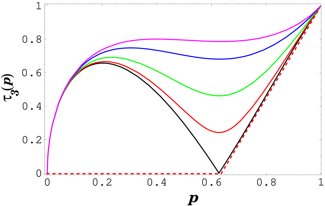
Figure 2: The 3-tangle of the states $\left|Z(p,\varphi)\right\rangle$ in Eq. (17) for various values of $\varphi=\gamma\cdot\frac{2\pi}{3}$ (from top to bottom: $\gamma=1/2,1/3,1/5,1/10,0$).

We have plotted $\tau_{3}(Z(p,\varphi))$ in Fig. 2 and its minimum (solid black line for $\varphi=0$)

$$\tilde{\tau}_{3}(p)\ = \ \min_{\varphi}\tau_{3}(Z(p,\varphi))$$ (21)

$$= \ \left|p^{2}-\frac{8\sqrt{6}}{9}\sqrt{p(1-p)^{3}}\right|\ \ .$$ (22)

The function $\tilde{\tau}_{3}(p)$ is not convex for $0\leq p\leq p_{0}$ and $0.825...\leq p\leq 1$. Its function convex hull, i.e., the convex characteristic curve for $\rho(p)$ in Eq. (16) is given by

$$\tau^{\ast}_{3}(p)=\left\{\begin{array}[]{ll}0\ \ ,&0\leq p\leq p_{0}\\ \tilde{\tau}_{3}(p)\ \ ,&p_{0}\leq p\leq p_{1}\\ 1-(1-p)\left(\frac{3}{2}+\frac{1}{18}\sqrt{465}\right)\ ,&p_{1}\leq p\leq 1\end{array}\right.$$ (23)

where

$$p_{1}\ =\ \frac{1}{2}\ +\ \frac{3}{310}\sqrt{465}\ =\ 0.70868\ldots$$ (24)

As we have explained in the preceding section $\tau^{\ast}(p)$ represents a lower bound for $\tau(\rho(p))$, and it coincides with the 3-tangle for those values $p$ for which the corresponding $\tau^{\ast}(p)$ is realized by at least one decomposition. For the states $\rho(p)$ it is not difficult to specify a decomposition with an average 3-tangle equal to $\tau^{\ast}(p)$ (see also Ref. Lohmayer et al. (2006)).

In the interval $p_{0}\leq p\leq p_{1}$ we have the “star-shaped” three-vector decomposition $\cal Z$

$$\rho(p)\ = \ \frac{1}{3}(\left|Z^{0}\right\rangle\!\left\langle Z^{0}\right|+\left|Z^{1}\right\rangle\!\left\langle Z^{1}\right|+\left|Z^{2}\right\rangle\!\left\langle Z^{2}\right|)$$ (25)

$$\left|Z^{0}\right\rangle\ = \ \sqrt{p}\left|GHZ\right\rangle\ -\ \sqrt{1-p}\left|W\right\rangle$$

$$\left|Z^{1}\right\rangle\ = \ \sqrt{p}\left|GHZ\right\rangle\ -\ e^{\frac{2\pi i}{3}}\sqrt{1-p}\left|W\right\rangle$$ (26)

$$\left|Z^{2}\right\rangle\ = \ \sqrt{p}\left|GHZ\right\rangle\ -\ e^{\frac{4\pi i}{3}}\sqrt{1-p}\left|W\right\rangle\ \ .$$

For $p\leq p_{0}$ a four-vector decomposition is optimal that combines the decomposition $\cal Z$ in Eq. (25) for $p_{0}$ with the W state:

$$\rho(p)\ =\ \frac{p}{p_{0}}\ \rho(p_{0})\ +\ \left(1-\frac{p}{p_{0}}\right)\ \pi_{\mathrm{W}}\ \ .$$ (27)

Finally, for $p_{0}\leq p\leq 1$, we need to combine the decomposition $\cal Z$ for $p_{1}$ with the GHZ state:

$$\rho(p)\ =\ \left(\frac{1-p}{1-p_{1}}\right)\ \rho(p_{1})\ +\ \left(\frac{p-p_{1}}{1-p_{1}}\right)\ \pi_{\mathrm{GHZ}}\ \ .$$ (28)

We stress that, as the convex characteristic curve $\tau^{\ast}_{3}(p)$ gives a strict lower bound for $\tau_{3}(\rho(p))$, the existence of decompositions attaining these values means that we have found the convex roof analytically. It is worth noticing that the above given optimal decomposition is unique.

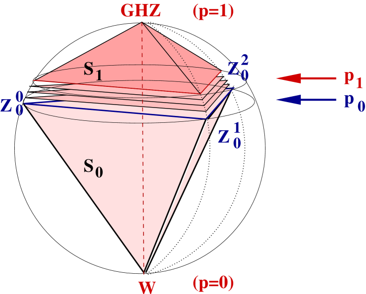
Figure 3: Bloch sphere for the two-dimensional space spanned by the GHZ state and the W state. The simplex $S_{0}$ contains all states with vanishing 3-tangle. The “leaves” between $p_{0}$ and $p_{1}$ represent sets of constant 3-tangle. In the simplex $S_{1}$, the 3-tangle is an affine function (for further explanation, see text).

The extension of the analytic convex roof to the entire simplices spanned by the decomposition vectors (see Fig 3) follows from the theorem that the vectors in an optimal decomposition are also optimal for the entire simplex they span (this applies also to states forming a subset of an optimal decomposition) Uhlmann (1998).

IV.2 Generic example for a rank-2 mixed two-qubit state

In the previous example we have seen that studying the convex characteristic curve may lead to a complete solution for the convex roof of a family of mixed states. In general, however, this may not be expected. The reason why the characteristic curve will typically fail to give the exact convex roof is because the phases $\varphi_{j}$ for which the minimum in Eqs. (11), (14) is reached, do not necessarily admit a decomposition of $\rho$.

Nevertheless one obtains valuable information about a given mixed state. In order to illustrate this, we describe a rather generic two-qubit case. Let us consider the states

$$\left|I\right\rangle\ = \ \frac{1}{\sqrt{5}}\ (2\left|00\right\rangle\ +\ \left|11\right\rangle)$$ (29)

$$\left|II\right\rangle\ = \ \frac{1}{\sqrt{6}}\ (\left|00\right\rangle+\left|01\right\rangle-2\left|11\right\rangle)$$ (30)

and their convex combinations

$$\rho_{2}(p)\ =\ p\ \pi_{I}\ +\ (1-p)\ \pi_{II}\ \ ,$$ (31)

We note that $\langle I|II\rangle=0$. This example can easily be treated analytically by using Wootters’ method Wootters (1998).

In particular, we find vanishing concurrence for $\tilde{p}_{0}=5/11$ (see Fig. 4).

Figure 4: Solid (blue) line: exact solution for the concurrence $C(\rho_{2}(p))$ according to Eqs. (29)–(31). For comparison: the convex characteristic curve of $\rho_{2}(p)$ (dashed red line; cf. also Fig. 5). The exact concurrence $C(\rho(p))$ has a zero for $\tilde{p}_{0}=5/11$.

Now let us first evaluate the zero-polytope (which is a line in the Bloch sphere in this case). The equation

$$C(\sqrt{p}\left|I\right\rangle+e^{i\varphi}\sqrt{1-p}\left|II\right\rangle)=0$$ (32)

has two real solutions for $p$: $\tilde{p}_{1}=5/29$ with $\varphi=\pi$ and $\tilde{p}_{2}=10/13$ with $\varphi=0$. ¿From this we can conclude immediately that there is exactly one value of $p$ for which the mixed-state concurrence of $\rho_{2}(p)$ vanishes: it is the intersection point of the zero-polytope with the line in the Bloch sphere that represents the family $\rho_{2}(p)$. Straightforward algebra shows that this intersection occurs at $\tilde{p}_{0}=5/11$.

We see that the zero-polytope indeed gives us exact information about a subset of the family $\rho_{2}(p)$ only (here: about a single element). Note however that this subset can even be empty in the most general case, when e.g. the wave function coefficients of (29) have a non-zero relative phase modulo $\pi$.

Figure 5: Concurrence for superpositions of states $\left|I\right\rangle$ and $\left|II\right\rangle$ (solid gray lines) and convex characteristic curve $C^{\ast}(p)$ (dashed red line). The convex characteristic curve coincides with the abscissa (i.e., $C^{\ast}(p)\equiv 0$) between the two zeros of Eq. (32), $\tilde{p}_{1}=5/29$ and $\tilde{p}_{2}=10/13$.

In Fig. 5 we show how the convex characteristic curve of $\rho_{2}(p)$ arises from the concurrence of superpositions of the states $\left|I\right\rangle$ and $\left|II\right\rangle$. Analytically, the convex characteristic curve reads:

$$C^{\ast}(p)=\left\{\begin{array}[]{ll}C_{-}(p)\ \ ,&0\leq p\leq\tilde{p}_{1}\\ 0\ \ ,&\tilde{p}_{1}\leq p\leq\tilde{p}_{2}\\ C_{+}(p)\ \ ,&\tilde{p}_{1}\leq p\leq 1\\ \end{array}\right.$$ (33)

where $C_{\pm}(p)=C(\sqrt{p}\left|I\right\rangle\pm\sqrt{1-p}\left|II\right\rangle)$. Clearly, $C^{\ast}(p)$ must vanish for all values of $p$ between the zeros according to Eq. (32). We observe (cf. Fig. 4) that $C^{\ast}(p)$ is indeed a lower bound to the exact concurrence. However, the latter is strongly underestimated by the convex characteristic curve for almost all $p$ values.

V Discussion

We have introduced two concepts that serve to facilitate the investigation of the convex roof of tangles for multipartite mixed qubit states. Both concepts are based on the tangle of pure-state superpositions, that is, of those pure states that lie in the range of the original density matrix.

The zero-polytope is formed by the convex set of density matrices with vanishing tangle in the range of the original mixed state under consideration. It can always be determined exactly. Then, the remaining task is the calculation of the convex roof for all remaining density matrices with non-zero tangle.

To this end, we have proposed the concept of the convex characteristic curve (or manifold). It leads to a non-trivial and possibly tight lower bound for the tangle of a given density matrix. In particular, it coincides with the convex roof if there is a decomposition of the original density matrix into pure states whose tangles lie on the convex characteristic curve.

In order to illustrate the power of these concepts we have discussed two simple examples – three-qubit mixed states with GHZ and W components Lohmayer et al. (2006), and a generic rank-2 two-qubit state. For the GHZ/W mixtures the convex characteristic curve shows analytically i) that the results of Ref. Lohmayer et al. (2006) indeed represent the convex roof for that family of states, and ii) provide an example where the convex characteristic curve provides the complete solution for a convex roof – namely, due to the fact that for each point of the convex characteristic curve there exists a decomposition that attains this lower bound. On the other hand, the two-qubit example displays that in a more general case, one may obtain non-trivial estimates for the convex roof. However, as in that case there hardly exists an optimal decomposition with all its elements on the convex characteristic curve, on must not expect that the obtained estimates for the convex roof are close to the exact value.

While, in principle, both concepts can be generalized to mixed states of arbitrary rank, their application is particularly adapted to the case of rank-2 states.

VI Acknowledgments

We would like to thank C. Eltschka and R. Lohmayer for stimulating discussions and helpful comments. This work was supported by the EU RTN grant HPRN-CT-2000-00144 and the Sonderforschungsbereich 631 of the German Research Foundation. J.S. receives support from the Heisenberg Programme of the German Research Foundation.

References

- Plenio and Virmani (2007) M. Plenio and S. Virmani, Quant. Inf. Comp. 7, 1 (2007).
- Uhlmann (1998) A. Uhlmann, Open Syst. Inf. Dyn. 5, 209 (1998), quant-ph/9704017.
- Wootters (1998) W. K. Wootters, Phys. Rev. Lett. 80, 2245 (1998).
- Uhlmann (2000) A. Uhlmann, Phys. Rev. A 62, 032307 (2000).
- Linden et al. (2006) N. Linden, S. Popescu, and J. A. Smolin, Phys.Rev.Lett 97, 100502 (2006).
- Cavalcanti et al. (2007) D. Cavalcanti, M. O. Terra Cunha, and A. Acin, Phys. Rev. A 76, 042329 (2007), quant-ph/0705.2521.
- Gour (2007) G. Gour (2007), arXiv:0707.1521.
- Niset and Cerf (2007) J. Niset and N. J. Cerf (2007), arXiv:0705.4650.
- Song et al. (2007) W. Song, N.-L. Liu, and Z.-B. Chen (2007), arXiv:0706.1598.
- Vidal (2000) G. Vidal, J.Mod.Opt. 47, 355 (2000).
- Bennett et al. (2000) C. H. Bennett, S. Popescu, D. Rohrlich, J. A. Smolin, and A. V. Thapliyal, Phys. Rev. A 63, 012307 (2000).
- Dür et al. (2000) W. Dür, G. Vidal, and J. I. Cirac, Phys. Rev. A 62, 062314 (2000).
- Verstraete et al. (2003) F. Verstraete, J. Dehaene, and B. D. Moor, Phys. Rev. A 68, 012103 (2003).
- Hill and Wootters (1997) S. Hill and W. K. Wootters, Phys. Rev. Lett. 78, 5022 (1997).
- Coffman et al. (2000) V. Coffman, J. Kundu, and W. K. Wootters, Phys. Rev. A 61, 052306 (2000).
- Leifer et al. (2004) M. S. Leifer, N. Linden, and A. Winter, Phys Rev A 69, 052304 (2004).
- Briand et al. (2003) E. Briand, J.-G. Luque, and J.-Y. Thibon, J. Phys. A 36, 9915 (2003).
- Osterloh and Siewert (2005) A. Osterloh and J. Siewert, Phys. Rev. A 72, 012337 (2005), quant-ph/0410102 on http://de.arxiv.org/.
- Osterloh and Siewert (2006) A. Osterloh and J. Siewert, Int. J. Quant. Inf. 4, 531 (2006), quant-ph/0506073 on http://de.arxiv.org/.
- Bennett et al. (1996) C. H. Bennett, D. DiVincenzo, J. A. Smolin, and W. K. Wootters, Phys. Rev. A 54, 3824 (1996).
- Benatti et al. (1996) F. Benatti, A. Narnhofer, and A. Uhlmann, Rep. Math. Phys. 38, 123 (1996).
- Schrödinger (1936) E. Schrödinger, Proc. Cambridge Phil. Soc. 32, 446 (1936).
- Lohmayer et al. (2006) R. Lohmayer, A. Osterloh, J. Siewert, and A. Uhlmann, Phys. Rev. Lett. 97, 260502 (2006).