The plasma picture of the fractional quantum Hall effect with internal SU() symmetries
Abstract
We consider trial wavefunctions exhibiting SU() symmetry which may be well-suited to grasp the physics of the fractional quantum Hall effect with internal degrees of freedom. Systems of relevance may be either spin-unpolarized states (), semiconductors bilayers () or graphene (). We find that some introduced states are unstable, undergoing phase separation or phase transition. This allows us to strongly reduce the set of candidate wavefunctions eligible for a particular filling factor. The stability criteria are obtained with the help of Laughlin’s plasma analogy, which we systematically generalize to the multicomponent SU() case. The validity of these criteria are corroborated by exact-diagonalization studies, for SU() and SU(). Furthermore, we study the pair-correlation functions of the ground state and elementary charged excitations within the multicomponent plasma picture.
pacs:
73.43.-f, 71.10.-w, 81.05.UwI Introduction
Soon after the discovery of the fractional quantum Hall effect (FQHE), Tsui Laughlin successfully described the underlying strongly-correlated electron liquid with the help of a simple trial wavefunction. Laughlin The reasons for the success of this approach were twofold: first, the calculated energy of this state is lower than that of charge-density waves or Wigner crystals,fukuyama which are natural candidates for the ground state within the partially filled lowest Landau level (LL) due to the quenched kinetic energy.Laughlin The second reason for its success is the fact that Laughlin’s wavefunction is in very sharp agreement with exact-diagonalization studies.EDlaughlin
A powerful tool in the understanding of Laughlin’s wavefunction is the quantum-classical analogy, in which its probability is interpreted as the (classical) Boltzmann weight of a two-dimensional (2D) one-component plasma (2DOCP).Laughlin Most strikingly, this analogy shows that Laughlin’s trial wavefunctions have no free parameter to be optimized by any variational calculation.
Laughlin’s original proposal was concerned with only one single species of fermions, namely spin-polarized electrons. In spite of its success, this is at first sight a very crude assumption in view of the relatively weak (effective) Zeeman effect when compared to the leading energy scale set by the Coulomb interaction , in terms of the magnetic length . Indeed the latter is almost two orders of magnitude larger than the bare spin splitting for typical magnetic fields of T. In order to account for an internal SU(2) spin symmetry, Halperin proposed a generalized trial wavefunction,Halperin which includes Laughlin’s as a special case. The latter may indeed be viewed as a Halperin wavefunction with a spontaneous ferromagnetic spin ordering.DasSarma
Halperin’s SU(2) wavefunctions have been a first step in the understanding of general multicomponent systems. In the case of bilayer quantum Hall systems, the same wavefunctions may be applied if one supposes a complete polarization of the physical spin and if one interprets the two layer indices as the two possible orientations of a pseudospin.DasSarma ; Moon However, the hypothesis of complete spin polarization is a priori as feably justified in bilayer as in monolayer quantum Hall systems, again due to a relatively weak Zeeman effect. A more appropriate approach is therefore one that takes into account the internal SU(4) spin-pseudospin symmetry. Such approaches have indeed been proposed in the description of ferromagnetic states when the LL filling factor , in terms of the electronic, , and the flux, , densities, respectively, is , or .ezawa ; arovas
Another example of a multicomponent quantum Hall system is graphene, where the internal SU(4) symmetry is due to the physical spin accompanied by a twofold valley degeneracy.GrapheneExp ; GrapheneTheo ; yang2 In contrast to the abovementioned bilayer quantum Hall systems, where the pseudospin symmetry is explicitely broken because of the difference between intra- and interlayer Coulomb interactions, the SU(4) symmetry is almost perfectly preserved in graphene from an interaction point of view – a possible (valley) symmetry breaking may be due to lattice effects, which are suppressed by the small parameter , where nm is the distance between nearest-neighbor carbon atoms in graphene, as compared to nm.Goerbig_Graphene ; AF ; Fuchs ; abanin ; Herbut In order to describe a possible, yet unobserved, FQHE in graphene, taking into account the appropriate form of the interaction potential, Nomura ; Goerbig_Graphene exact diagonalization studies have been performed in the framework of an internal SU(2) valley symmetry,Apalkov ; Toke as well as in a SU(4) composite-fermion approach.yang ; toke
More recently, two of us have proposed a generalization of Halperin’s wavefunctions to components, i.e. systems with an internal SU() symmetry, in order to describe a possible FQHE in -component systems, namely graphene with .Goerbig_SU4 Here, we investigate the stability of these wavefunctions from two complementary perspectives – first, we derive stability criteria within a generalized plasma picture. This analogy allows one to interpret the SU() Halperin wavefunctions in terms of correlated 2DOCP and to describe in a compact manner their ground-state properties as well as the elementary excitations with fractional charge. In a second step, we corroborate the validity of the generalized plasma picture with the help of exact-diagonalization studies.
After a brief review of Laughlin’s plasma analogy (Sec. II), we generalize the plasma picture to -component systems in Sec. III. In Sec. IV, we derive general stability criteria within the plasma analogy, on the basis of which we discuss the stability of specific SU(2) and SU(4) wavefunctions. We complete this paper with a discussion of ground-state properties, such as sum rules for the pair correlation functions (Sec. V), and fractional charges of quasiparticle/-hole excitations (Sec. VI).
II Laughlin’s Plasma Analogy
In order to describe a correlated electron liquid to account for the FQHE, Laughlin proposed the -particle trial wavefunctionLaughlin
| (1) |
where denotes the position of the -th electron in the complex plane. Here and in the following, we set the magnetic length , for notational convenience. The form of this trial wavefunction is solely determined by the analyticity condition for the lowest LL – i.e. all single-particle states are of the form , where is a positive integer – and by symmetry considerations. In order to have a translational and rotational invariant state and thus an incompressible state with no gapless Goldstone mode, the wavefunction may only depend on the relative distance of the -th and the -th particle. Furthermore, fermion statistics for electrons requires the exponent to be an odd integer, which is the only variational parameter of Laughlin’s wavefunction (1).
However, the parameter turns out to be fixed by the electon density, or else the filling factor, , as Laughlin showed with the help of a plasma analogy.Laughlin Indeed, one may interpret the modulus square of the wave function as the Boltzmann weight
| (2) |
of a classical system, namely a 2DOCP described by the classical HamiltonianLaughlin ; OCP ; Bhatta
| (3) |
where one has set somewhat arbitrarily the inverse ”temperature” . Notice that the true temperature does not intervene in the analysis because the system is placed at . The first term describes 2D interacting particles of charge , whereas the second term may be interpreted as a homogeneous background of charge (jellium). The minimization of the classical Hamiltonian corresponds, via the relation (2), to a maximal quantum probability of the original quantum system of electrons within the lowest LL. The classical ground state of the Hamiltonian (3), however, is obtained when the plasma particles of charge are fully neutralized by the background, i.e. when
| (4) |
It is evident from the last equation that the variational parameter must be positive – otherwise one would have to treat with unphysical negative densities. Notice that from the wavefunction point of view, is not physical because it violates the analyticity condition for wavefunctions in the lowest LL. This point, which may seem obvious, is worth being emphasized and being recalled in the following sections when the plasma picture is generalized to more components.
III Plasma Picture for SU() Halperin wavefunctions
Based on Halperin’s idea to write down a Laughlin-type wavefunction for a two-component quantum Hall system, in order to take into account the spin degree of freedom,Halperin two of us have proposed a SU() generalization for a -component system,Goerbig_SU4
| (5) | |||||
There are different types of electrons [denoted with superscript ] with inter- () and intra-component () quantum correlations, and is the complex position of -th electron of type . The lowest-LL analyticity condition imposes that all exponents, and , must be integers. Furthermore, must be odd in the case of fermions. Apart from , discussed by Halperin,Halperin wavefunctions may be physically significant in the case of bilayer quantum Hall systems and graphene. In the former example, the internal degrees of freedom do not only contain the physical SU(2) spin (), but also a layer index, which may be mimicked by an additional SU(2) isospin (). There are thus four internal states, , , , and . In the case of graphene, an isospin () must be introduced in order to account for the two-fold valley degeneracy. Wavefunctions similar to those in Eq. (III) have been proposed by Qiu et al. for multilayer quantum Hall systems,Qiu by Morf as potential candidates for the FQHE hierarchy states,morf and by Yang et al. in the study of a possible FQHE in graphene.yang
Again, the starting point of the plasma analogy is Eq. (2), and one associates the new Hamiltonian with a physical system. In the case , this system has been interpreted as a generalized plasma, which consists of different particle types (each of which corresponds to a different electron type in the original quantum system) plus a neutralizing background.Girvin_Correlation ; DasSarma With the identification (2), one obtains for the wavefunctions (III) the classical Hamiltonian
| (6) | |||||
Here the first term represents a sum over 2D interaction terms for -type particles of charge , whereas the second one takes into account interactions between particles of different type, and . However, this generalized plasma does not satisfy the charge superposition principleJackson unless , which is a rather special case.
Instead of one single plasma of types of particles, it seems therefore more appropriate to interpret this generalized plasma in terms of different 2DOCPs (one for each type of electrons) with correlations between them. For this purpose, we introduce the continuum limit, in which the density for particles of type (electrons or plasmatic particles) is . In order to distinguish the resulting Hamiltonian from the original discrete one, we supress the subscript in Eq. (3), and one obtains the energy functional
| (7) |
Here, is the symmetric exponent matrix, with and ,Goerbig_SU4 and is the surface occupied by the plasma. Similarly to the one-component case, the configurations with maximal probability [Eq. (2)] are obtained by minimizing with respect to all densities. The stationary points are found at
| (8) |
In order to have a minimum, the Hessian matrix
| (9) |
which is identical to the exponent matrix up to a positive constant, needs to be positive, i.e. have positive eigenvalues. One may interpret Eq. (8) as the stationary point of a 2DOCP of ()-type particles, whereas the positions of all other particles of type () are fixed and constitute a quasi-static impurity potential felt by the ()-type particles. For the 2DOCP of this type, the interactions between all other types of particles yields only an unimportant constant, with respect to the derivative. In this sense, one may indeed interpret the system as correlated 2DOCPs rather than a single plasma of different types of particles.
In the same manner as for a single 2DOCP, Eq. (8) is satisfied when each of the plasmas exhibits quasi-neutrality,Bhatta but now contributions from the impurities have to be taken into account,
| (10a) | |||
| (10h) | |||
Here, on the r.h.s. of Eq. (10a) represents the neutralizing background, as for a single 2DOCP [Eq. (4)]. The second term in Eq. (10a) represents the contributions from type-() particles due to inter-component correlations. One notices that Eq. (10h) is the matrix generalization of Eq. (4). This result was previously derived by counting the zeros of the wavefunction (III).Goerbig_SU4 Invertible matrices yield a unique solution with all densities being uniform, , as it is the case for U() Laughlin’s liquid. The case of non-invertible matrices will be discussed in the next section.
Unlike the U() case, fixing the total filling factor does not determine uniquely the exponent matrix. It has been pointed out in Ref. Goerbig_SU4, that several candidate wavefunctions may give rise to a FQHE at the same filling factor , especially in the case of larger internal symmetry groups. Moreover, even if one fixes all component filling factors , the wavefunction is not unambiguous. As an example, we consider the SU() Halperin wavefunctions (), with (i) , [(331) wavefunction], and (ii) , [(113) wavefunction]. Both wavefunctions describe a situation with and have been considered in the past within the study of a possible unpolarized state.Yoshioka Indeed, an even-denominator quantum Hall state has been observed at and , in the first excited LL.5_2 However, it is strongly unlikely that this state is spin-unpolarizedmorf2 ; pan ; halperin07 and more sophisticated theories, in terms of a Pfaffian state, need to be invoked to account for a spin-polarized state.theory5_2 As we will show below, stability conditions related to Eq. (9) allow one, in the case of unpolarized states, to discriminate between () and () wavefunctions, for .
IV Stability
In order to obtain a stable state, the stationary point obtained from Eq. (8) must be a minimum, i.e. the Hessian matrix in Eq. (9) must be positive. Otherwise, the plasmas would not be stable, or else in the state of lowest energy. Hence, a first stability condition imposes that all eigenvalues of must be positive.
There is indeed a limiting case for which one, or more, eigenvalue(s) is (are) zero. Because the potential is quadratic, the minimum point becomes now a line of minima, which correspond to different ground states. If at least one eigenvalue is zero, the exponent matrix is no longer invertible, and all densities may not be fully determined from Eq. (10h).
This point may alternatively be interpreted in terms of SU() ferromagnets – different states of equal energy may, e.g., occur at various combinations of two (or more) filling factors and , although the sum is fixed. In this case one may introduce a pseudo-spin operator , which can possibly take all values in between . The simplest example of such a case is the Laughlin wavefunction with an internal spin degree of freedom [a Halperin () wavefunction], which is, for odd , completely antisymmetric in its orbital part. For fermions, the spin wavefunction must therefore be completely symmetric and represents thus a SU() ferromagnet. If the total spin is oriented along the positive direction, all electrons reside in the upper spin branch (, ). In the absence of a Zeeman effect, this state has the same energy as the one with a total spin in the direction (, ), as well as any intermediate state with . In the general SU() case, the ferromagnetic properties are determined by the rank of the matrix . Indeed, if and one introduces common fixed filling factors for the relevant components, one may describe the resulting state by a SU() Halperin wavefunction with an invertible exponent matrix with additional pseudo-spin degrees of freedom for the components the density of which remain undetermined.Goerbig_SU4
As mentioned earlier, some exponent matrices can lead to negative density solutions for Eq. (10h). A second class of stability conditions needs to be imposed in order to prevent this unphysical situation, which may occur even in the case of a positive matrix .
In order to illustrate the two conditions, we discuss some specific examples for different . The case has already been presented above.
IV.1 The case
We first study Halperin’s wavefunction () for the SU() case, which is described by the exponent matrix
Even if all exponents are positive, as required by the lowest-LL analyticity condition, the eigenvalues and the filling factors are not necessarily so,
| (11a) | |||
| (11b) | |||
In order to obtain only positive eigenvalues (first stability condition), one needs to require
| (12) |
The case corresponds to a situation of a non-invertible matrix of rank . Because of Eq. (12), positive densities (filling factors) are found from Eq. (11b) only for
| (13) |
which we thus need to impose as a second class of stability conditions. One furthermore notices form Eqs. (12) and (13) that the only states with a non-invertible exponent matrix of rank are the ferromagnetic Laughlin states () discussed above.
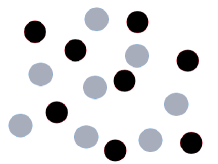
The final stability criterion Eq. (13) for SU() wavefunctions has a compelling physical interpretation: intra-component must always be stronger than inter-component correlations. Within the plasma picture, this may also be understood from Figs. 1, 2(a), and 2(b). For illustration, we consider the () wavefunction, where is left as a variable, which we treat in a rather artificial manner as a continuous variable in the following discussion. It is evident that only integer values may be taken into account for physical candidate wavefunctions.

(a)
|
(b)

|
Fig. 1 shows the plot of both component filling factors and the lower eigenvalue, . This graph can be split into three distinct parts I,II, and III.
-
•
Part I (). Each type-() particle carries a charge and is affected by those from the type-() plasma through a charge coupling of , which may be interpreted as constituting a quasi-static impurity distribution interacting with type-() particles. Alternatively, one may concentrate on type-() particles with charge , which see type-() particles as a distribution of charge impurities. Therefore both types of particles are more strongly repelled by those of their own species than by particles of different type. One thus obtains a stable homogeneous mixture of two plasmas, which is shown in Fig. 2(a).
-
•
Part II (). Although type-() particles are still more strongly repelled by those of their own species than by type-() particles (), this is not the case for type-() particles. Because their inter-species repulsion is now weaker than that which they experience from type-() particles (), they prefer to gather rather than to be mixed to type-() particles. This indicates a tendency to phase-separate, and the effect manifests itself in an unphysical negative filling factor . The divergence of the filling factors at the artificial value of in Fig. 1 is due to the vanishing of the eigenvalue . Above , the original minimum of the energy functional (7) evolves into a saddle point, and the first stability condition of non-negative eigenvalues is no longer satisfied. Indeed, one notices that the filling factors interchange their role – although the repulsion between type-() particles is stronger than that between type-() particles and one would therefore intuitively expect that , one finds for .
-
•
Part III (). Above , the inter-component repulsion is stronger than that between particles of like type. The phase separation between the two plasmas, which we have alluded to in the discussion of part II, is well-pronounced. Due to this strong inter-component repulsion, the interface between the two plasmas needs to be minimized, and this results in an inhomogeneous state of two spatially separated plasmas, as shown in Fig. 2(b). Should the partial densities not be fixed, i.e. particles could flip from to state, it is clear that the system would favor a distribution where only one type of particles would remain. The interface between the two plasmas disappears.

Fig. 3 shows the stability graph for the a wavefunction (here with ). In this case, the eigenvalues (11a) and the component filling factors (11b) become
| (14) |
respectively. Although the component filling factors remain positive for all choices of , the eigenvalue becomes negative for , where one would expect a phase separation between the two plasmas, as in the case of the () wavefunction [Fig. 2(a)]. The critical value corresponds to the Laughlin case with a SU(2) ferromagnetic spin wavefunction, discussed above. For the case , both trial wavefunctions, () and (), are valuable candidates for the description of a potential FQHE at if only the symmetry considerations for trial wavefunctions in the lowest LL are taken into account. However, the plasma analogy indicates clearly that only one of the two wavefunctions, namely (), yields a stable physical state. At half-filling, e.g., the only SU(2) Halperin wavefunction which might yield a stable FQHE state is (), whereas corresponds to an unstable plasma, which is not evident from wavefunction calculations alone.Yoshioka
IV.2 The case
We now consider generalized Halperin wavefunctions with an internal SU() symmetry. We restrict our studies to a particular subset of the latter, noted (), the corresponding exponent matrices of which may be written asGoerbig_SU4
| (15) |
If applied to graphene, those correlation coefficients imply that one treats all intervalley components () on the same footing and intravalley ones separately (, for and valley, respectively). This is an even more natural assumption in the case of bilayer quantum Hall systems in semiconductor heterostructures, where interlayer correlations (described by the exponents ) are weaker than intralayer ones ( and which couple the different spin orientations within the and layer, respectively). Moreover, some intracomponent correlations are fixed to the same value for explicit calculation of the eigenvalues and filling factors to be carried out. However, we will only settle here the conditions for all quantities to be positive (first and second stability arguments), and these conditions are satisfied if
| (16) |
The case where one of the two first inequalities, or the two last, turn into an equality corresponds to matrices of rank . For Eq. (16) becomes an equation set and, once again, the only stable state is of Laughlin-type () with SU()-ferromagnetic ordering. The stability criteria [Eq. (16)] yield a slightly more complex interpretation: not only do intracomponent correlations have to be stronger than some intercomponent ones but there are also conditions between intercomponent coefficients. This may be more easily understood within the () state, where is left as a variable, similarly to the SU(2) case discussed in Sec. IV A. Again, we have chosen this state purely for illustration reasons.
Fig. 4 plots all filling factors and the relative signed eigenvalue . As for the case , the graph is split into parts I,II and III.

-
•
Part I (). One notices that type-() and () particles act identically therefore one can virtually treat the problem as for the case . Type-() and () plasmas are stable separately, with respect to the previous section on SU() wavefunctions. Moreover, type-() particles carry a charge and are affected by type-() quasi-static impurities of charge. Similarly, type-() particles with charge interact with type-() plasma through a charge. Hence, one plasma suffers weaker repulsion from the other and type-() and () will mix in order to form a stable homogeneous state.
-
•
Part II (). The eigenvalue is now negative () as well as some filling factors. In the plasma picture, type-() particles are equally repelled by their own species and type-() quasi-static impurities, each carrying a charge. On the contrary, the type-() plasma still experiences more ”favourable” repulsion from type-() particles. One cannot conclude about the stability at this level and some care has to be taken of the inner composition of the type-() particles. Indeed, type-() particles cary a charge and interacts with type-() quasi-static impurities via a charge which is less than any other charge for this plasma. Similarly, type-() will be less repelled by type-() particles than by any other particles. Hence, type-() plasma will tend to phase separate, which is contradictory to the phase mixing tendency of type-() particles. As in the case, this yields unphysical negative densities for type-() particles.
-
•
Part III (). Above , all filling factors are positive but becomes more and more negative. For , the same argument as above can be developped: type-() plasma tend separate from type-(), whereas type-() tend to mix with type-(). Surprisingly, this is not related to a negative density, as in any other case previoulsy discussed. This may be due to the composite nature of type-() plasma. For , both plasma are more severely repelled by each other such that the phase separation is complete.
IV.3 Comparison with Exact-Diagonalization Studies
The stability discussed so far is only related to the particular form of the wavefunctions and it has somehow to be linked to the true ground-state of the quantum system with interacting electrons. We therefore investigate the stability of generalized Halperin wavefunctions within exact-diagonalization studies. The system is mapped onto a sphere in the center of which a magnetic monopole is fixed to ensure a magnetic field orthogonal to the surface. This magnetic monopole creates flux quanta threading the surface of the sphere. At a particular filling factor , the relation between the number of particles and that of flux quanta is
where
| (17) |
and the shift
| (18) |
is due to the finite-size geometry and depends on the particular wavefunction considered.
All calculations are performed within the lowest LL, with the help of Haldane’s pseudopotentials,Haldane , which determine the interaction between two electrons of type and with a relative angular momentum . Halperin’s wavefunctions represent the exact ground-state for a model interaction such that
| (21) | |||||
| (24) |
One of the simplest non-trivial cases occurs when all intra-(inter-)component correlations are the same, i.e. and . These states are fully unpolarized and the corresponding filling factor and shift are
| (25) |
respectively. We have already shown in Sec. IV A and Sec. IV B that, within the plasma picture, yields a stable and an unstable state, whereas represents a (stable) Laughlin state with SU() ferromagnetic order. This stability criterion may also be obtained directly from the interaction model corresponding to the -Halperin state: whenever this state is unstable, other zero-energy states with respect to the model interaction appear in the fully polarized sectors. These zero-energy states are quasihole excitations of the -Laughlin state the model interaction of which matches that of the Haperin state in that sector. This is a direct consequence of for unstable states, as may be seen from Eq. (25) with . Thus any Zeeman-type perturbation or any extra pseudopotentials beyond the model interaction dramatically change the polarization, as suggested by the plasma picture. For more generic Halperin wave functions, similar conclusions can be drawn when one of the is lower than .
When the polarization is regarded as fixed, the phase separation is clearly observed through the study of pair correlation function, which are discussed in Sec. V B. As mentionned before, unstable systems will rather exhibit the instability through unphysical correlation functions.Forrester
In addition to these general stability arguments, we investigate via exact diagonalization the , () and () wavefunctions studied by Yoshioka et al.Yoshioka The first state is realized for the particular model , all other potentials being zero, and . The second one is related to and . For electrons, and correspondingly and flux quanta, exact-diagonalization calculations yield an energy gap of for () as compared to for (). Hence, the () state has an energy gap which is almost two orders of magnitude smaller than the characteristic energy, which is set to one. One may therefore expect that the () state is much less stable than the () state, as indicated by the plasma analogy and the abovementioned argument. This is indeed the case as may be seen when other pseudopotentials are chosen non-zero in a perturbative manner. We choose, for this investigation, to vary continuously and from zero to one, in the case of the () state, and and for (). Our exact-diagonalization results show that the unpolarized state described by the abovementioned wavefunctions (there is an equal number of spin and ) is conserved only for the () case. Moreover, there is indeed an instability of the () state such that even a small perturbation in the pseudpotentials ( for example) completely polarizes the state, in agreement with the general polarization argument given above.
(a)
(b)
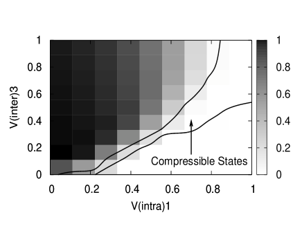
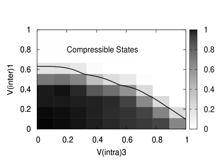
We now focus on the unpolarized sector although the system is no more in its ground-state in the () case. The unpolarized sector may be physically relevant for a system with constrained polarizations such as for a bilayer configuration with equal densities in both layers. Fig. 5 presents phase diagrams with compressible and incompressible states for () and () varying states. The overlap between the exact ground-state and the Halperin wavefunctions is represented by gradual shading. For the () case, it can be observed that there is a finite energy gap around the values of the exact model, and the overlap between the true ground state and the trial wavefunction remains large whenever the pseudopotentials and remain in this area. Further increase of the potentials leads to a gap collapse at relatively large values of the pseudopotentials. Hence, this state is stable even in the case of more realistic interactions beyond the model situation.
In the case of the () wavefunction, the gap collapses rapidly even at small values of (). A rather subtle perturbation would therefore completely change the system since a zero energy gap is incompatible with any FQHE. Outside the funnel-shaped area of compressible states, cf. Fig. 5(b), the overlap can be either quite small (, at larger values of and ) or quite large (, in the vicinity of the model situation). This indicates that the incompressible states are described by states with different symmetry. However, even though the system appears as stable up to relatively high , the gap remains small ( to ). Moreover we emphasize that, in the case of an unfixed polarization, the ground state is no longer in the unpolarized sector.
Notice that the phase diagram in Fig. 5(b) is not generic for all unstable wavefunctions, but may be attributed to the pathologic model interaction of . General considerations on stability should only treat the polarization and pair correlation functions arguments.
In the same manner as for the case , we compare the plasma picture with exact-diagonalization results for . For the special subset of matrices previously discussed, it has been checked numerically that unstable states are related to the existence of partially polarized zero-energy states with a lower number of flux quanta. As in the case , those states will be favored when any Zeeman-like perturbation is introduced. The phase transition predicted within the plasma picture is recovered. We checked this criterion for several particular wavefunctions, such as () and (), and it appears that wavefunctions with unstable corresponding plasma do polarize, partially or completely, in agreement with the classical stability discussed in Sec. IV B. For a given fixed polarization, phase separation is likely to be observed, as in the case.
V Ground State Properties
Although the plasma picture is a powerful tool for the study of intrinsic properties of Laughlin and generalized Halperin wavefunctions, as shown in the previous section, it gives in itself no indication of the physical state chosen by the true interaction Hamiltonian. The Hamiltonian (6) is obtained from a formal mapping of the wavefunctions to a corresponding plasma model, but it is not related to the original Hamiltonian of interacting particles in the lowest or partially filled higher LL. Indeed, incompressible quantum liquids, which display the FQHE, are not found at all possible filling factors for which one may write down a trial wavefunction. E.g. in the lowest LL, a Wigner crystal is energetically favorable at ,lam in the first excited LL a succession of FQHE states and Wigner and bubble crystalsgoerbigRIQHE gives rise to a reentrant integral quantum Hall effect,eisenstein and in even higher LLs stripe phasesFKS ; moessner yield a highly anisotropic longitudinal transport.expStripes Which of these competing phases is indeed chosen depends on the precise form of the true interaction of electrons in a fixed partially filled LL.
It is however possible to express the energy of Laughlin’s wavefunction in terms of the 3D Coulomb interaction potential and the pair correlation function
apart from a normalization constant,
| (26) |
The plasma picture may be of use here because the pair correlation functions for electrons and for plasmatic particles are the same, as may be seen from Eq. (2). The pair correlation function may be expanded asGirvin_Correlation
| (27) |
where the prime indicates a sum only over odd (due to Fermi statistics), and the expansion parameters vanish in the large- limit. These expansion parameters are constrained in several respects. First, the short-range behavior implies that for . Second, particular properties of the logarithmic potential in the plasma picture can be used to derive sum rules, which act as further constraints.Baus ; OCP ; GMP ; Kalinay
V.1 Sum rules for SU() pair correlation functions
For wavefunctions with SU() symmetry, there are pair correlation functions if all densities are well-defined, i.e. if is invertible. The correlation function between type-() and type-() electrons is denoted by , and one may generalize the expression (27) to the case of -component wavefunctions,
| (28) |
where the expansion coefficients vanish for large . Here, the prime indicates summation over odd only for the intra-species functions . Indeeed, Fermi statistics is no more relevant when considering distinguishable electrons of type and . As for the Laughlin () case, the short-range behavior implies that for .
Further sum rules may be derived within the picture of correlated plasmas introduced in the previous section. In order to derive those in the simplest manner, we decouple the different plasmas with the help of an orthogonal transformation on the densities,
| (29) |
which diagonalizes the exponent matrix, , in terms of the orthogonal matrix . The diagonalized Hamiltonian thus reads
| (30) | |||||
where is the -th eigenvalue of and . The Hamiltonian is a sum of independent Hamiltonians , each of which corresponds to a single 2DOCP. The correlation functions for these plasmas must therefore obey the usual sum rules for 2DOCPsBaus ; OCP ; Kalinay
| (31a) | |||||
| (31b) | |||||
| (31c) | |||||
| (31d) | |||||
for the different moments
Here, primes indicate quantities in the diagonal basis. Eq. (31a) is due to the charge neutrality of the system, Eq. (31b) reflects its perfect-screening property, and Eq. (31c) is a compressibility sum rule. The third moment [Eq. (31d)] has no apparent physical interpretation. Because the plasmas are decoupled in the diagonal basis, there are no correlations between different plasmas, i.e. for .
The pair correlation functions in the original basis may be obtained from the with the help of the inverse orthogonal transformation. It is useful to start from the definition of the structure factor in reciprocal space, which is related to the pair correlation function by Fourier transformation,
for the simplest case. It may also be expressed in terms of density operators,
| (32) |
where the quantities in brackets are averages with respect to the probability density function. In the case of , the structure factor has a matrix form,
and the associated pair correlation functions may be obtained from those in the diagonal basis with the help of ,
| (33) |
The sum rules (31a) to (31d) for the diagonal basis thus immediatly yield those for the correlated 2DOCP, due to Eq. (33). For instance, the zeroth- and the first-moment rules are
| (34a) | |||||
| (34b) | |||||
respectively. Eqs. (34a) and (34b) are generalizations of results, which have previously been obtained for .Girvin_Correlation ; Forrester Second- and third-moment rules may be derived in the same manner.
V.2 Exact-diagonalization results for pair correlation functions


The pair correlation functions of the ground-state may also be obtained from exact-diagonalization results. We first focus on the SU(2) case by considering the same () and () wavefunctions discussed above and studied by Yoshioka et al.Yoshioka As mentioned in Sec. IV C, the first state is realized for the particular model , all other potentials being zero, and . The second one is related to and . Fig. 6(a) shows the ground-state pair correlation functions for the state with electrons and flux quanta, and the results for the case ( and ) are displayed in Fig. 6(b). The correlation function of a pair of electrons is the relative density of type- electrons when a type- electron is fixed at the origin, . With this definition in mind, one can infer that the (331) state is rather well-behaved. Correlation functions vanish near the origin, as a result of repulsive interactions and Fermi statistics. The density peaks at finite distances indicate different layers of electrons (on average) with regular alternation of particles of type () and (). The large-distance limit of type- particles is related to a uniform density. Hence, the system discussed is composed of a uniform and homogeneous mix of electrons of both types. Unlike this first case, the state displays a vanishing intra-component function () at large distances. Electrons of both types thus tend to aggregate on a finite-size location. Moreover, the inter-component function () is maximum only at infinity which implies that the different types of electrons tend to spatially separate. This corroborates the plasma picture of phase-separated particles.


We now turn to the SU(4) case by considering the two stable generalized Halperin wave functions studied in Ref. Goerbig_SU4, , namely (3333,111) and (3333,033). The correlation functions are computed for electrons and flux quanta. While the partial filling factors of the (3333,111) state are fixed and all equal to , only the filling factor per layer is fixed for the (3333,033) ferromagnetic state. For a better comparison, we have set the partial filling factors to be the same as those of (3333,111). Thus in both cases, there are only two electrons per species leading to prominent finite size effect ( is out of computational reach). The (3333,111) state is the straightforward SU(4) generalization of (331) and is therefore similar to its SU(2) counterpart (bearing in mind the small system size we are considering). The (3333,033) state consists of two independent spin insensitive Laughlin states in each layer. Both intra-layer and intra-component correlation functions are therefore identical to their Laughlin counterpart (up to normalization factors). The inter-layer pairs are trivially constant in this non-correlated layer (3333,033) state.
Furthermore, we have confirmed numerically the validity of the sum rules (34a) and (34b) for the SU(2) and SU(4) states discussed above. Notice that in the state may be described alternatively by a SU(2) wavefunction, where the two components correspond to the two layer indices, regardless of the spin orientation. The relevant sum rules are therefore those of the SU(2) case, in which the exponent matrix in Eq. (34b) is invertible.
VI Charged Excitations
In this section, we study the charged excitations of SU() Halperin wavefunctions with the help of the plasma analogy. For , quasi-hole excitations of the Laughlin wavefunction may be written as
| (35) |
They consist of adding a zero of density, or a magnetic flux, in the electron liquid at the position .
Within the plasma picture, the extra Jastrow term adds a new potential term to the Hamiltonian (3),
| (36) |
which thus describes a 2DOCP with a fixed impurity at and charge . Because of the plasma’s perfect screening ability,Bhatta the particles are rearranged so that they screen the effect of the impurity in its vicinity. This requires particles in the plasma picture such that in the true electron liquid, the real charge of the excitation must be
| (37) |
in units of the electron charge. Hence one electron can screen excitations.
We now investigate SU() Halperin wavefunctions for which there exist different types of excitation. The quasi-hole wavefunction
| (38) |
creates here an excitation of ()-type electrons at the position , i.e. adds a magnetic flux in the ()-th component of the electron liquid. The modified Hamiltonian in the plasma picture contains a new potential of an impurity that only affects particles of type (),
Each of the correlated 2DOCP exhibits perfect screening ability, i.e. the plasma of type () must screen the impurity totally,
| (39) |
whereas plasmas of type (), with , screen a zero impurity
| (40) |
Here, is the quasiparticle charge, in units of the electron charge, carried by electrons of type () in the electron liquid for excitations in the () component. Eqs. (39) and (40) were previously derived for the case,DasSarma and one may write them in a concise matrix form as
| (41) |
The last equation is valid only if is invertible. Indeed, if this is not the case, some component densities remain unfixed, as described in the previous section, and one could only consider excitation of groups of particles with a definite density. For instance, the () Halperin wavefunction has a non-invertible exponent matrix; the densities and may fluctuate although their sum remains fixed, . Physical excitation must therefore not distinguish between the two components.
For the case, (3333,111) wavefunctionGoerbig_SU4 exhibit four excitation types each of which carries a charge, whereas for the (3333,033) wavefunction, only joined ()-() and ()-() excitations are to be considered, each of charge .
Tab. 1 shows examples of charged excitations for SU() wavefunctions.
| n | |||||||
|---|---|---|---|---|---|---|---|
| 3 | 3 | 0 | 2/3 | 1/3 | 0 | 0 | 1/3 |
| 3 | 3 | 1 | 1/2 | 3/8 | -1/8 | -1/8 | 3/8 |
| 1 | 1 | 3 | 1/2 | -1/8 | 3/8 | 3/8 | -1/8 |
| 3 | 3 | 2 | 2/5 | 3/5 | -2/5 | -2/5 | 3/5 |
| 2 | 2 | 3 | 2/5 | -2/5 | 3/5 | 3/5 | -2/5 |
| 3 | 3 | 3 | 1/3 | 1/3 | |||
The first example describes two independent Laughlin states and it is consistent that a type-() excitation should only affect type-() particles. The four next examples are related to the ”() and ()” problem. One should notice that there are inconsistencies for () and () states. Indeed, when an extra flux quantum is added to the type-() component, the number of flux quanta increases by one and the electron density remains the same. Therefore, the filling factor should decrease. However the total charge is conserved, so the sign of the quasi-hole charge should be the same as that of the electron, in order to compensate this ”electronic” lack. This is not the case for () and () states which must be thus considered as unphysical, in addition to the conclusions drawn in the previous sections. The last example in Tab. 1 is simply a Laughlin wavefunction split into two arbitrary sets. There is only one common excitation, as for the usual U() case.
Similarly, Tab. 2 shows some charged excited states for SU() wavefunctions.
| 3333,111 | 2/3 | 1/6 | 1/6 | 1/6 | 1/6 |
|---|---|---|---|---|---|
| 3555,222 | 2/5 | 1/5 | 1/15 | 1/15 | 1/15 |
| 3535,222 | 8/19 | 3/19 | 1/19 | 3/19 | 1/19 |
| 5555,222 | 4/11 | 1/11 | 1/11 | 1/11 | 1/11 |
All examples are associated with invertible matrices . No proof is given here, but we conjecture that unstable states yield some inconsistencies concerning the charged excitations, as for the case.
VII Conclusions
In conclusion, we have investigated the stability of Halperin wavefunctions for -component quantum Hall systems, with a particular emphasis on the cases and . The associated SU(2) and SU(4) internal symmetries happen to be the physically most relevant if one considers, e.g., bilayer quantum Hall systems and graphene in a strong magnetic field. The case occurs when the Zeeman effect is relatively small with respect to the leading interaction energy scales. In order to derive the stability criteria, we have generalized, in a systematic manner, Laughlin’s plasma analogy to multicomponent systems. The validity of the criteria is corroborated with the help of exact-diagonalization studies.
As for the conventional one-component quantum Hall system, the quantum-classical analogy yields a compelling physical interpretation of the trial wavefunctions, in terms of correlated 2DOCP. Besides the stability of the trial wavefunctions, it also allows one to understand relevant ground-state properties, such as the associated pair-correlation functions, and fractionally charged quasiparticle excitations.
Whether the discussed trial wavefunctions correctly describe the true ground state in physically relevant multicomponent systems, such as bilayer quantum Hall systems or graphene, depends on the precise form of the interaction potential. The plasma analogy with its rather artificial interaction may not give insight here, and variational or exact-diagonalization studies need to be performed to determine the correct ground state for a physical interaction potential. It has indeed been shown that in the case of Coulomb interaction, a possible FQHE state at is not described by a generalized SU() Halperin wavefunction.toke ; Goerbig_SU4 More complicated trial wavefunctions, such as composite-fermiontoke or even more exotic states, may describe FQHE states at this and possibly other filling factors in a more appropriate manner. However, in the U(1) one-component quantum Hall system, the inevitable starting point in the understanding of the FQHE is Laughlin’s wavefunction;Laughlin other wavefunctions may be viewed as sophisticated generalizations of it. In the same manner, the study of SU() Halperin wavefunctions and the plasma analogy yield important physical insight into multicomponent quantum Hall systems, and one may conjecture that they play a similar basic role for possible generalizations as Laughlin’s in the U(1) case.
Furthermore, it has been shown in the SU(2) case, that not all possible, though stable from our analysis, Halperin wavefunctions are valid candidates from a symmetry point of view. Indeed, most of the () wavefunctions are not eigenstates of the total spin operator, the Casimir operator of SU(2), as they should for spin-independent interaction Hamiltonians.prange The (331) wavefunction discussed here, is, e.g., not an eigenstate of the total spin. However, this problem may be cured by attaching the permanent of the matrix to the (331) wavefunction.prange ; HR The situation is more complicated in the SU(4) case, where there are more Casimir (spin-pseudospin) operators, and the wavefunctions should be eigenstates of these operators. More detailed theoretical investigations are required to settle the question whether some SU(4) wavefunctions may be corrected in a similar manner.
Acknowledgments
We acknowledge fruitful discussions with J.-N. Fuchs, P. Lederer, R. Morf, and S. H. Simon. This work has partially been funded by the Agence Nationale de la Recherche under Grant Nos. ANR-06-NANO-019-03 and ANR-07-JCJC-0003-01.
References
- (1) D. C. Tsui, H. L. Störmer, and A. C. Gossard, Phys. Rev. Lett. 48, 1559 (1982).
- (2) R. B. Laughlin, Phys. Rev. Lett. 50, 1395 (1983).
- (3) H. Fukuyama, P. M. Platzman, and P. W. Anderson, Phys. Rev. B 19, 5211 (1979).
- (4) F. D. M. Haldane and E. H. Rezayi, Phys. Rev. Lett. 54, 237 (1985); G. Fano, F. Ortolani, and E. Colombo, Phys. Rev. B 34, 2670 (1986).
- (5) B. I. Halperin, Helv. Phys. Acta 56, 75 (1983).
- (6) For a review see: S. M. Girvin and A. H. MacDonald, in Perspectives in Quantum Hall Effects, edited by S. Das Sarma and A. Pinczuk (John Wiley, New York, 1997).
- (7) K. Moon, H. Mori, K. Yang, S. M. Girvin, A. H. MacDonald, I. Zheng, D. Yoshioka et S.-C. Zhang, Phys. Rev. B 51, 5138 (1995).
- (8) Z. F. Ezawa, Phys. Rev. Lett. 82, 3512 (1999); Quantum Hall Effects: Field Theoretical Approach and Related Topics (World Scientific, 2000).
- (9) D. P. Arovas, A. Karlhede, and D. Lilliehöök, Phys. Rev. B 59, 13147 (1999).
- (10) K. S. Novoselov, A. K. Geim, S. V. Morosov, D. Jiang, M. I. Katsnelson, I. V. Grigorieva, S. V. Dubonos, and A. A. Firsov, Nature 438, 197 (2005); Y. Zhang, Y.-W. Tan, H. L. Stormer, and P. Kim, Nature 438, 201 (2005).
- (11) V. P. Gusynin and S. G. Sharapov, Phys. Rev. Lett. 95, 146801 (2005); Phys. Rev. B 73, 245411 (2006); N. M. R. Peres, F. Guinea, A. H. Castro Neto, Phys. Rev. B 73, 125411 (2006).
- (12) For a review of the quantum Hall effect in graphene, see K. Yang, Solid State Comm. 143, 27 (2007).
- (13) M. O. Goerbig, R. Moessner, and B. Douçot, Phys. Rev. B 74, 161407(R) (2006).
- (14) J. Alicea and M. P. A. Fisher, Phys. Rev. B 74, 075422 (2006).
- (15) J.-N. Fuchs and P. Lederer, Phys. Rev. Lett. 98, 016803 (2007).
- (16) D. A. Abanin, P. A. Lee, and L. S. Levitov, Phys. Rev. Lett. 98, 156801 (2007).
- (17) I. F. Herbut, Phys. Rev. B 75, 165411 (2007); Phys. Rev. B 76, 085432 (2007).
- (18) K. Nomura and A.H. MacDonald, Phys. Rev. Lett. 96, 256602 (2006).
- (19) V. M. Apalkov, and T. Chakraborty, Phs. Rev. Lett. 97, 126801 (2006).
- (20) C. Töke, P. Lammert, V. H. Crespi, and J. K. Jain, Phys. Rev. B 74, 235417 (2006).
- (21) K. Yang, S. Das Sarma, and A. H. MacDonald, Phys. Rev. B 74, 075423 (2006).
- (22) C. Töke and J. K. Jain, Phys. Rev. B 75, 245440 (2007).
- (23) M. O. Goerbig, and N. Regnault, Phys. Rev. B 75, 241405(R) (2007).
- (24) J. M. Caillol, D. Levesque, J. J. Weiss, and J. P. Hansen , J. Stat. Phys. 28, 325 (1982).
- (25) D. A. Gurnett, and A. Bhattacharjee, Introduction to Plasma Physics, (Cambridge University Press, 2005).
- (26) X. Qiu, R. Joynt, and A. H. MacDonald, Phys. Rev. B 40, 1943 (1989).
- (27) R. Morf, private communication.
- (28) S. M. Girvin, Phys. Rev. B 30, 558 (1984).
- (29) J. D. Jackson, Classical Electrodynamics, (Wiley Publication, 2005).
- (30) A. H. MacDonald, D. Yoshioka, and S. M. Girvin, Phys. Rev. B 39, 8044 (1989).
- (31) R. L. Willett, J. P. Eisenstein, H. L. Stormer, A. C. Gossard, and J. H. English, Phys. Rev. Lett. 59, 1776 (1987).
- (32) R. Morf, Phys. Rev. Lett. 80, 1505 (1998).
- (33) W. Pan, H. L. Stormer, D. C. Tsui, L. N. Pfeiffer, K. W. Baldwin, and K. W. West, Solid State Commun. 119, 641 (2001).
- (34) I. Dimov, B. I. Halperin, C. Nayak, arXiv:0710.1921.
- (35) G. Moore and N. Read, Nucl. Phys. B 360, 362 (1991).
- (36) F. D. M. Haldane, Phys. Rev. Lett. 51, 605 (1983).
- (37) P. J. Forrester, and B. Jancovici, J. Phys. Lettres 45,L-583 (1984)
- (38) P. K. Lam and S. M. Girvin, Phys. Rev. B 30, 473 (1984); 31, 613(E) (1985).
- (39) M. O. Goerbig, P. Lederer, and C. Morais Smith, Phys. Rev. B 68, 241302 (2003); ibid. 69, 115327 (2004).
- (40) J. P. Eisenstein, K. B. Cooper, L. N. Pfeiffer, and K. W. West, Phys. Rev. Lett. 88, 076801 (2002); J. S. Xia, W. Pan, C. L. Vicente, E. D. Adams, N. S. Sullivan, H. L. Stormer, L. N. Pfeiffer, K. W. Baldwin, and K. W. West, Phys. Rev. Lett. 93, 176809 (2004).
- (41) A. A. Koulakov, M. M. Fogler, and B. I. Shklovskii, Phys. Rev. Lett. 76, 499 (1996); M. M. Fogler, A. A. Koulakov, and B. I. Shklovskii, Phys. Rev. B 54, 1853 (1996).
- (42) R. Moessner and J. T. Chalker, Phys. Rev. B 54, 5006 (1996).
- (43) M. P. Lilly, K. B. Cooper, J. P. Eisenstein, L. N. Pfeiffer, and K. W. West, Phys. Rev. Lett. 82, 394 (1999); R. R. Du, D. C. Tsui, H. L. Stormer, L. N. Pfeiffer, K. W. Baldwin, and K. W. West, Solid State Commun. 109, 389 (1999).
- (44) M. Baus, and J. P. Hansen, Phys. Rep. 59, 1 (1980).
- (45) S. M. Girvin, A. H. MacDonald, and P. M. Platzman, Phys. Rev. B 33, 2481 (1986).
- (46) P. Kalinay, P. Markos̆, L. S̆amaj, and I. Travĕnec, J. Stat. Phys. 98, 639 (2000).
- (47) S. M. Girvin, in The Quantum Hall Effect, edited by R. E. Prange and S. M. Girvin (Springer-Verlag, New York, 1987).
- (48) F. D. M. Haldane and E. H. Rezayi, Phys. Rev. Lett. 60, 956 (1988).