Self-diffusion of Rod-like Viruses Through Smectic Layers

Abstract

We report the direct visualization at the scale of single particles of mass transport between smectic layers, also called permeation, in a suspension of rod-like viruses. Self-diffusion takes place preferentially in the direction normal to the smectic layers, and occurs by quasi-quantized steps of one rod length. The diffusion rate corresponds with the rate calculated from the diffusion in the nematic state with a lamellar periodic ordering potential that is obtained experimentally.

Since the pioneering work of Onsager on the entropy driven phase transition to a liquid crystalline state Onsager , the structure and the phase behavior of complex fluids containing anisotropic particles with hard core interactions has been a subject of considerable interest, both theoretically rodsTheo and experimentally rodsExp . Understanding of the particle mobility in the different liquid crystalline phases is more recent simulations . In experiments various methods have been applied to obtain the ensemble averaged self-diffusion coefficients in thermotropic NMRthermo and amphiphilic NMRlyo liquid crystals, block copolymer Fredrickson96 and colloidal systems FRAP . Only a few studies have been done where dynamical phenomena are probed at the scale of a single anisotropic particle: the Brownian motion of an isolated colloidal ellipsoid in confined geometry ellipsoid and the self-diffusion in a nematic phase formed by rod-like viruses EPLpavlik represent two recent examples. In the latter case, the diffusion parallel ($D_{\|}$) and perpendicular ($D_{\bot}$) to the average rod orientation (the director) has been measured, showing an increase of the ratio $D_{\|}/D_{\bot}$ with particle concentration. Knowledge of the dynamics at the single particle level is fundamental for understanding the physics of mesophases with spatial order like the smectic (lamellar) phase of rod-like particles. In this mesophase the particle density is periodic in one dimension parallel to the long axis of the rods, while the interparticle correlations perpendicular to this axis are short-ranged (fluid-like order). For parallel diffusion to take place, the rods need to jump between adjacent smectic layers, overcoming an energy barrier related to the smectic order parameter deGennes . This process of interlayer diffusion, or permeation, was first predicted by Helfrich Helfrich . In this Letter, we use video fluorescence microscopy to monitor the dynamics of individual labeled colloidal rods in the background of a smectic mesophase formed by identical but unlabeled rods. In this way we directly observe permeation of single rods in adjacent layers. As in the nematic phase, self-diffusion in a smectic phase is anisotropic: the diffusion through the smectic layers is shown here to be much faster than the diffusion within each liquid-like layer, i.e. $D_{\|}/D_{\bot}\gg 1$, in contrast to thermotropic systems. Moreover, since the individual rod positions within the layer are monitored, the potential barrier for permeation is straightly determined for the first time. The permeation can then be described in terms of Brownian particles diffusing in a one-dimensional periodic symmetric potential.

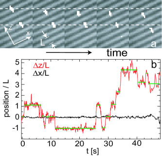
Figure 1: (a) Time sequence of an overlay of fluorescence and DIC images showing labeled particles jumping between adjacent smectic layers ($\Delta t=0.071s$ is the time between two frames). The layer spacing is $L\simeq 0.9~{}\mu m$. (b) Displacement of a given particle in the direction parallel (red) and perpendicular (black) to the director. The green lines indicate the residence time, i.e. the time for which one particle stays in a given layer.

The system of rods used in this work consists of filamentous bacteriophages fd, which are semi-rigid polyelectrolytes with a contour length of 0.88 $\mu m$, a diameter of 6.6 nm, and a persistence length of 2.2 $\mu m$ protocol . Suspensions of fd rods in aqueous solution form several lyotropic liquid crystalline phases, in particular the chiral nematic (cholesteric) phase and the smectic phase Revuefd . The existence of a smectic phase in suspensions of hard rods is an evidence of the high monodispersity and therefore of the model system character of such filamentous viruses SmPoly ; KRP-PRE2007 . The colloidal scale of the fd bacteriophage facilitates the imaging of individual rods by fluorescence microscopy, as well as smectic layers by differential interference contrast (DIC) microscopy Revuefd . Fig. 1(a) shows a sequence of images of a single region protocolVideo where both techniques are combined. A comparison of the images shows that some rods jump between two layers while others remain within a given layer. The trajectory of one of the rods is plotted in Fig. 1(b) in the direction parallel (z) and perpendicular (x) to the director. This figure summarizes the key observation of this Letter: the diffusion throughout the smectic layers takes place in quasi-quantized steps of one rod length i.e. the mass transport between the layers is a discontinuous process. Moreover, it shows that the diffusion within the smectic player is extremely slow note .

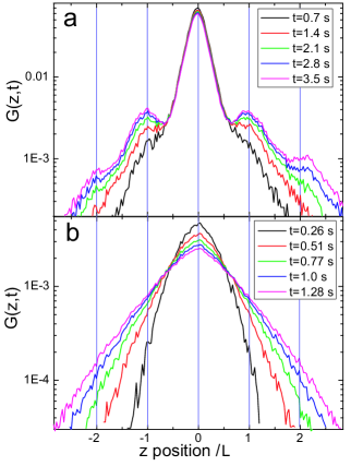
Figure 2: Probability density function in space at different times for two ionic strengths: 20 mM (a) and 110 mM (b). The functions are normalized to one, the z-axis is scaled by the smectic layer thickness $L$.

The “hopping-type” diffusion is mainly the consequence of the underlying ordering potential of the smectic phase and the vacancies available in adjacent layers. A phenomenological expression for permeation has been derived by coupling the displacement of a segment of a smectic layer $u$ to the compressibility modulus $\tilde{B}$ via the permeation parameter $\lambda_{b}$ deGennes :

$$\frac{\partial u}{\partial t}=\lambda_{b}\tilde{B}\frac{\partial^{2}u}{\partial z^{2}}.$$ (1)

On a single-particle level, the fundamental solution of this diffusion equation is the self-van Hove function VanHove , which is the probability for a displacement $z$ during a time $t$:

$$G(z,t)=\frac{1}{N}\sum_{i=1}^{N}\delta[z+z_{i}(0\frac{}{})-z_{i}(t)].$$ (2)

Since single particles are experimentally identified, the self-van Hove function can be directly obtained from the histogram of particle positions after a time $t$, as plotted in Fig. 2 for low (I = 20 mM) and high ionic (I = 110 mM) strengths. For a fluid made of Brownian particles, a smooth gaussian distribution that smears out over time is expected for the self-van Hove function. However at low ionic strength, $G(z,t)$ shows distinct peaks exactly at integer multiples of the particle length (and therefore of the layer thickness, see Fig. 2(a)) as expected from visual observation (Fig. 1). At high ionic strength the curves are smoother (Fig. 2(b)), but in all cases the experimental self-van Hove function is not gaussian at any time. This implies that the permeation parameter $\lambda_{b}$ in Eq. 1 is a function of position $z$, due to the energy landscape imposed by the smectic layers.

The energy landscape can be determined experimentally from the distribution of particle positions with respect to the middle of a layer parallel to the director. To this end, time windows are selected where the particle remains for ten frames or more within the same layer. The distribution of particles within a single layer is then obtained by addition of all particle positions relative to the average position of particles for all selected time windows. The resulting distributions are plotted in Fig. 3(a) for the two ionic strengths. To obtain the total particle distribution for the full smectic phase, the distributions of particles in a single layer (Fig. 3(a)) is added periodically to itself at all integer numbers of layer spacing $L$ (Fig. 1(a)). The smectic ordering potential is then deduced from the Boltzmann factor $P(z)\sim e^{-U_{layer}(z)/k_{B}T}$ for the probability of finding a particle at position $z$, as shown in Fig. 3(b). Both potentials can be best fitted with a sinusoidal $U_{layer}(z)=U_{0}\sin(2\pi z/L)$, giving an amplitude of $U_{0}=1.36\;k_{B}T$ at low ionic strength and $U_{0}=0.66\;k_{B}T$ at high ionic strength. The difference between the two amplitudes explains the fact that for I = 20 mM the self-van Hove function exhibits discrete peaks, while for I = 110 mM the potential barrier is small enough to exhibit a monotonic behavior of the probability density function. The reason for the more pronounced potential at low ionic strength might be that electrostatic interactions between rods are more long-ranged, i.e., particles are more strongly correlated so that it is more difficult to create a void between them. The fact that the potential can be fitted by a sinusoidal is remarkable by itself. Indeed, the use of such a potential is very common due to its simplicity SmTheo , but this ordering potential has never been directly observed until now. Moreover the height of the potential, i.e. the smectic order parameter, can be directly obtained.

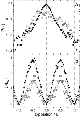
Figure 3: (a) Histogram of time averaged particle positions parallel to the director within the smectic layer at 20 mM ($\blacksquare$) and 110 mM ($\circ$). The histogram is normalized by the total number of positions. (b) Resulting effective mean ordering potential in the z-direction obtained by applying the Boltzmann factor. The solid lines are a fit to a sinusoidal potential.

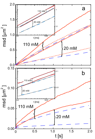
Figure 4: (a) Mean square displacement parallel to the director for the two indicated ionic strengths in the nematic phase (red line), in the smectic phase (blue dashed line), and in the nematic phase considering the oscillatory potential (red dotted line). (b) Mean square displacement perpendicular to the director (same convention as above). The insets show the same data in a log-log scale, yielding the degree of subdiffusion from the linear regression (black line).

The overall mean square displacement (MSD) of rods parallel and perpendicular to the director of the smectic and nematic phase is plotted in Fig. 4 for both ionic strengths. The time evolution of the MSD given by $\langle\Delta r^{2}(t)\rangle\sim t^{\gamma}$ provides the diffusion exponent $\gamma$: $\gamma<1$ is characteristic of a subdiffusive behavior, while $\gamma>1$ is referred to as superdiffusion. The parallel motion is close to be diffusive ($\gamma\simeq 1$) in both the nematic ($\gamma=0.97$) and smectic ($\gamma=0.94$) phases for I = 110 mM and in the nematic phase for I = 20 mM ($\gamma=0.95$). Only the parallel motion in the smectic phase for low ionic strength, i.e. where the discrete peaks in the self-van Hove function are observed, is significantly subdiffusive: $\gamma=0.81$. The perpendicular motion is in all cases strongly subdiffusive: for I = 110 mM, $\gamma$ reduces from 0.63 before to 0.56 after the nematic-smectic (N-Sm) transition and for I = 20 mM it reduces from 0.68 to 0.46. Anomalous subdiffusive behavior has often been observed in systems where diffusion takes place by steps, e.g. in case of release from a surrounding cage cage . This “cage escape” might be at the origin of the observed subdiffusive behavior for both parallel and perpendicular diffusion. For parallel diffusion the cage is formed by the energy barrier imposed by the smectic layers, as shown by smaller $\gamma$ for higher ordering potential. Perpendicular diffusion at high volume fractions is only possible through a reptation-like motion along the long axis to escape the local excluded volume, as observed for polymers for which typically $\gamma=0.5$ McLeish02 . This excluded volume is huge, even for thin rods at high orientational order, due to the large rod aspect ratio of $\approx 130$. In addition, perpendicular diffusion in the smectic phase is hindered due to the ordering potential, which couples this diffusion to the permeation and which thus explains the decrease of $\gamma$ from the nematic to the smectic phases. For subdiffusive systems, a non-Gaussian distribution of the probability density functions has been observed as in Fig. 2 cage , even though these two features are not a priori correlated. Note also that boundary effects might influence the probability density wall .

The anisotropy in the total diffusion, $D_{\|}/D_{\bot}$, which is about 20 in the nematic phase EPLpavlik , increases in the smectic phase as a result of the pronounced subdiffusivity of the perpendicular motion (decrease of $\gamma$). These observations show an opposite trend as compared to thermotropic liquid crystals simulations ; NMRthermo , where usually $D_{\|}/D_{\bot}$ evolves from being larger than one at temperatures close to the N-Sm transition temperature to being smaller than one at lower temperatures sm . Therefore the diffusion in the smectic phase can be effectively considered as a one-dimensional diffusion of a Brownian particle in a periodic potential in the high friction limit. A general expression for such a diffusion process is given by Festa78 :

$${D_{\|}}=\frac{D_{0}}{\langle e^{-U_{layer}(z)/k_{B}T}\rangle\langle e^{U_{layer}(z)/k_{B}T}\rangle}.$$ (3)

The brackets indicate averaging over one period of the ordering potential. The diffusion coefficient in the smectic phase can then be calculated taking $D_{0}$ as the diffusion coefficient in the nematic phase close to the N-Sm transition, and using $U_{layer}$ as obtained from the fit of the potentials plotted in Fig. 3: the diffusion coefficient decreases by a factor 0.84 at I = 110 mM and by a factor 0.44 at I = 20 mM. Indeed the MSD in the smectic phase is obtained from the MSD in the nematic phase, using these factors for both ionic strengths (see Fig. 4), although at I = 20 mM some deviation appears due to the subdiffusivity in the MSD. Thus, we have shown how the mobility of rods decreases after the N-Sm transition, contrary to the isotropic-nematic transition where the global mobility increases due to entropic gain Onsager ; EPLpavlik . It seems therefore to indicate that fd virus suspensions do not behave as a system of rigid hard rods for high concentration in agreement with a recent work KRP-PRE2007 . Moreover, the very slow diffusion within the layers suggests that the smectic phase of semi-flexible colloidal rods consists of layers of glass-like, rather than fluid-like, particles.

In conclusion, we have for the first time visualized the process of permeation in the smectic phase at the scale of single particles for a system of charged rods. This allowed us to give a full and coherent description of the diffusion process without any assumptions on the system. The diffusion is strongly anisotropic in the direction normal to the smectic layers and quasi-discontinuous due to the presence of the layers. The parallel diffusion rate complies with the rate in the nematic phase, taking into account the ordering potential, which is obtained directly from our measurements.

We thank Jan Dhont for fruitful discussions. This project was supported by the European network of excellence SoftComp. MPL acknowledges also the SFB TR6 for financial support.

References

- (1) L. Onsager, Ann. N.Y. Acad. Sci. 51, 627 (1949).
- (2) D. Frenkel et al., Nature 332, 822 (1988); G.J. Vroege, H.N.W. Lekkerkerker, Rep. Prog. Phys. 55, 1241 (1992).
- (3) X. Wen et al., Phys. Rev. Lett. 63, 2760 (1989); H. Maeda and Y. Maeda, Phys. Rev. Lett. 90, 018303 (2003); Z. Dogic and S. Fraden, Curr. Opin. Colloid Interface Sci., 11, 47 (2006).
- (4) S. Hess et al., Molec. Phys. 74, 765 (1991); H. Löwen, Phys. Rev. E 59, 1989 (1999); R.L.B. Selinger, Phys. Rev. E 65, 051702 (2002); M.A. Bates, G.R. Luckhurst, J. Chem. Phys. 120, 394 (2004); M. Cifelli et al., J. Chem. Phys. 125, 164912 (2006).
- (5) G.J. Krüger, Phys. Rep. 82, 229 (1982); S.V. Dvinskikh et al., Phys. Rev. E 65, 061701 (2002); J. Xu et al, Phys. Rev. E 72, 051703 (2005).
- (6) R. Blinc et al., Phys. Rev. Lett. 25, 1327 (1970); S. Gaemers and A. Bax, J. Am. Chem. Soc 123, 12343 (2001); P.L. Hubbard et al., Langmuir, 21, 4340 (2005); Y. Gambin et al., Phys. Rev. Lett. 94, 110602 (2005).
- (7) G.H. Fredrickson and F.S. Bates, Annu. Rev. Mater. Sci. 26, 501 (1996).
- (8) Z. Bu et al., Macromolecules 27, 6871 (1994); M.P.B. van Bruggen et al., Phys. Rev. E 58, 7668 (1998); R. Cush and P.S. Russo, Macromolecules 35, 8659 (2002).
- (9) Y. Han et al., Science, 314, 626 (2006).
- (10) M.P. Lettinga et al., Europhys. Lett. 71, 692 (2005).
- (11) P.G. de Gennes and J. Prost, The Physics of Liquid Crystals (Clarendon, Oxford, 1993).
- (12) W. Helfrich, Phys. Rev. Lett. 23, 372 (1969).
- (13) fd was grown using the XL1-Blue strain of E. Coli as the host bacteria and purified following standard biological protocols Revuefd . To vary the ionic strength, viruses have been dialyzed against a 20 mM TRIS-HCl buffer at pH = 8.2 with an adjusted amount of NaCl. About one fd out of 104 has been labeled with the dye Alexa-488 (Invitrogen).
- (14) Z. Dogic and S. Fraden, in Soft Matter, edited by G. Gompper and M. Schick (Wiley-VCH, Weinheim, 2006), Vol. 2.
- (15) M.A. Bates and D. Frenkel, J. Chem. Phys. 109, 6193 (1998).
- (16) K.R. Purdy and S. Fraden, Phys. Rev. E 76, 011705 (2007).
- (17) The time resolution of the used CCD camera (Hamamatsu C9100) was between 10 and 120 ms, depending on the region of interest.
- (18) To quantify this hopping-type diffusion, the jumps have been identified with a home-written algorithm based on the criterion that the first N positions in time should deviate in one direction from the previous average, and that the distance between two jumps should be close to the particle length.
- (19) J.P. Hansen and I.R. McDonald, Theory of Simple Liquids (Academic Press, London, 1986).
- (20) B. Mulder, Phys. Rev. A 35, 3095 (1987); A. Stroobants et al., Phys. Rev. Lett. 57, 1452 (1986).
- (21) E. R. Weeks and D. A Weitz, Phys. Rev. Lett. 89, 095704 (2002); ibid. Chemical Physics 284, 361 (2002).
- (22) T. C. B. McLeish, Advances in Physics 51, 1379 (2002).
- (23) Although data acquisitions were always taken in the middle of the sample which is rather thin (about ), the diffusion has been observed to slow down close to the cell walls.
- (24) The interpretation of such behaviors is ambiguous due to the different temperature dependence of the viscosity parallel and perpendicular to the director.
- (25) R. Festa and E. Galleani d’Agliano, Physica, 90a, 229 (1978).