Critical behavior of diluted magnetic semiconductors: the apparent violation and the eventual restoration of the Harris criterion for all regimes of disorder

Abstract

Using large-scale Monte Carlo calculations, we consider strongly disordered Heisenberg models on a cubic lattice with missing sites (as in diluted magnetic semiconductors such as $\textrm{Ga}_{1-x}\textrm{Mn}_{x}\textrm{As}$). For disorder ranging from weak to strong levels of dilution, we identify Curie temperatures and calculate the critical exponents $\nu$, $\gamma$, $\eta$, and $\beta$ finding, per the Harris criterion, good agreement with critical indices for the pure Heisenberg model where there is no disorder component. Moreover, we find that thermodynamic quantities (e.g. the second moment of the magnetization per spin) self average at the ferromagnetic transition temperature with relative fluctuations tending to zero with increasing system size. We directly calculate effective critical exponents for $T>T_{c}$, yielding values which may differ significantly from the critical indices for the pure system, especially in the presence of strong disorder. Ultimately, the difference is only apparent, and eventually disappears when $T$ is very close to $T_{c}$.

I Introduction

Technologically relevant magnetic materials such as diluted magnetic semiconductors (DMS) are characteristically strongly disordered due to the low concentration of random magnetic moments (e.g. $\textrm{Ga}_{1-x}\textrm{Mn}_{x}As$ where 5% - 12 % of the Ga sites are occupied by substituent Mn ions). DMS materials such as $\textrm{Ga}_{1-x}\textrm{Mn}_{x}\textrm{As}$ have been modeled theoretically using a classical Heisenberg model on an fcc lattice where the Hamiltonian is $\mathcal{H}=\sum_{i,j}J_{ij}\mathbf{S}_{i}\cdot\mathbf{S}_{j}$ with $J(r_{ij})$ being a carrier (hole) mediated random indirect exchange coupling between moments separated by a distance $r_{ij}$ given by $J(r)=J_{0}e^{-r/l}r^{-4}[\sin(2k_{\mathrm{F}}r)-2k_{\mathrm{F}}r\cos(2k_{\mathrm{F}}r)]$. $k_{\mathrm{F}}=(\frac{3}{2}\pi^{2}n_{c})^{1/3}$ is the Fermi wave number, $n_{c}$ is the hole density, and $l$ is the damping scale.

While individual parameters such as the ferromagnetic transition temperature $T_{c}$ have been calculated in theoretical studies DJP1 ; DJP2 , the critical behavior of strongly disordered Heisenberg models on a three dimensional lattice has not been understood in detail in the context of a direct numerical calculation. At the ferromagnetic transition, thermodynamic quantities scale as power laws in the reduced temperature $t=(T-T_{c})/T_{c}$ with, e.g., the magnetization varying as $m\propto t^{\beta}$, the correlation length scaling as $\xi\propto t^{-\nu}$, and $\chi\propto t^{-\gamma}$ for the magnetic susceptibility; hence critical exponents such as $\beta$, $\nu$, and $\gamma$ (up to prefactors specific to the model under consideration) completely specify the critical behavior near $T_{c}$ where $t\ll 1$.

Our task is to determine the extent to which the critical behavior of the three dimensional Heisenberg model is influenced by disorder (in the form of randomly removed magnetic moments), and we have found the most singular contributions to critical behavior to be unaffected by disorder whether only a few magnetic moments are removed or the majority of magnetic impurities are missing in cases of strong disorder. A theoretical result (derived from a renormalization group calculation) known as the Harris criterion Harris holds that the sign of the specific heat exponent $\alpha$ determines whether the critical exponents are altered. Specifically, although modifications in the universality class are expected for $\alpha>0$, the Harris criterion predicts that disorder will not affect the critical exponents when $\alpha<0$. The hyper-scaling identity $\alpha=2-d\nu$ implies that the condition for stable critical behavior is $\nu>2/d$, $d=3$ being the dimensionality of our system. In particular, since $\nu=0.714>0.67$ for the Heisenberg model Peli , the Harris result precludes disorder induced shifts in the critical exponents. With careful finite size scaling analysis, we have indeed confirmed that critical behavior in the disordered models conforms to the 3D Heisenberg universality class. An important finding of our detailed numerical study is, however, the fact that the effective critical exponents of the strongly disordered model may very well manifest an apparent violation of the Harris criterion (i.e. a deviation from the corresponding pure Heisenberg model values) away from the critical temperature, thus possibly considerably complicating the interpretation of experimental data.”

The results of our numerical calculations are consistent with experiment where the local critical behavior of thermodynamic quantities such as the magnetic susceptibility $\chi$ (e.g. the slope $\gamma_{\mathrm{eff}}=d\log(\chi)/d\log(t)$ of the log-log plot in the case of the magnetic susceptibility) differ from the critical indices of the pure case with $c=1.0$ for intermediate values of the reduced temperature. Ultimately, the effective critical exponents converge for sufficiently small $t$ to the critical behavior of the model with no disorder. Similarly, we examine finite size systems, and we would obtain results for critical behavior which differ from those of the pure model if we extrapolate to the bulk limit in naïve manner. However, by taking into account corrections to scaling, we compensate for finite size effects and obtain critical exponents identical to those of the pure Heisenberg model.

Using large-scale Monte Carlo simulations, we calculate critical exponents for the disordered Heisenberg model on a 3D lattice. Hence, we show that the universality class remains unaltered from regimes where the model is weakly disordered and only a few magnetic moments are removed to cases such as $c=0.4$ (the site percolation threshold for the simple cubic lattice is $c=0.3116$ where on average fewer than half of the magnetic ions participate in a ferromagnetically ordered phase).

Another component of the Harris criterion is the prediction that thermodynamic variables such as the magnetization $m$ and magnetic susceptibility $\chi$ do (do not ) self-average at $T_{c}$ in the bulk limit when $\nu>(<)2/3$. The extent of self-averaging may be quantified via the parameter $g_{2}=([\langle m^{2}\rangle^{2}]-[\langle m^{2}\rangle]^{2})/[\langle m^{2}\rangle]^{2}$ g2 , the relative variance of $[\langle m^{2}\rangle]$ with respect to disorder where $m$ is the magnetization, angular brackets indicate thermal averages, and square brackets refer to disorder averaging. For the Heisenberg model, we find self-averaging to be intact with $g_{2}$ ultimately decreasing after reaching a maximum for moderate sized systems containing on the order of a few hundred magnetic impurities.

In Section II, we discuss details of our numerical techniques for determining critical behavior of the disordered Heisenberg model. Subtleties include the need for a careful calculation of the Curie Temperature $T_{c}$, and taking into account corrections to scaling which would otherwise lead to the conclusion that disorder has affected the critical behavior of the Heisenberg model; we find that the universality class is not influenced by disorder, being identical to that of the pure model.

In Section III, we give results in tabular form for the critical exponents obtained in our calculation. Explicit numerical values are given for the critical indices $\nu$, $\beta$, $\gamma$, and $\eta$ for disorder ranging from very weak (e.g. $c=0.95$) to quite strong (i.e. $c=0.4$). In each case, we also provide the corresponding critical exponent (calculated by us) for the pure model, which is consistent with the best and most recent values given in the literature.

In Section IV, we provide the apparent critical exponents which differ from those of the pure model, and would be obtained for system sizes that are not sufficiently large. Similarly, if one is not close enough to $T_{c}$ in experiment (generally, the reduced temperature $t=(T-T_{c})/T_{C}$ should be less than $10^{-3}$ to obtain the critical exponents of the pure Heisenberg model in systems with disorder), spurious apparent critical indices will be measured. This apparent violation of the Harris criterion, even very slightly away from the critical temperature, is an important cautionary remark following directly from our Monte Carlo studies of the disordered model.

Finally, in the Appendix (Section V), we provide the Monte Carlo numerical results for thermodynamic variables such as the magnetization $m$ and magnetic susceptibility $\chi$. Also included are the corresponding theoretical results taking into account leading singular terms, as well as the first correction to scaling. There is very good agreement between the Monte Carlo data and the results of the theoretical model (i.e. generally at least one part in $10^{3}$ or better).

II Methods and Techniques in the Numerical Analysis

Singularities in variables such as the specific heat and magnetic susceptibility are smoothened as $t\rightarrow 0$ and the correlation length $\xi$ becomes comparable to the system size $L$. However, we can determine critical exponents by exploiting finite size scaling at $T_{c}$; the magnetization scales at $m\propto L^{-\beta/L}$, the thermal derivative $d\xi/dT$ of the correlation length $\xi$ varies as $d\xi/dT\propto L^{1/\nu}$, and the magnetic susceptibility $\chi$ diverges with increasing system size $L$ with the singular dependence $\chi=cL^{3}([\langle m^{2}\rangle]-[\langle m\rangle]^{2})\propto L^{\gamma/\nu}$. The critical exponents $\nu$, $\beta/\nu$, and $\gamma/\nu$ are obtained by calculating the appropriate thermodynamic quantities for many different system sizes and carefully extrapolating to the thermodynamic limit. Having calculated $\nu$, $\gamma$, and $\beta$, one may obtain additional critical exponents such with the aid of hyperscaling relations. As an example, the exponent $\eta$, given in terms of $\gamma$ and $\nu$ by $\eta=2-\gamma/\nu$, is useful because it is a more sensitive parameter than $\gamma$ alone in gauging the universality class of a specific model.

To obtain critical exponents accurately, it is essential that calculations be performed as close as possible to $T_{c}$ Chen since the temperature range where finite size scaling holds becomes narrower with increasing system size $L$. To obtain the ferromagnetic transition temperature $T_{c}$ as precisely as possible, we numerically calculate the normalized correlation length $\xi/L$ following reference Kim . For temperatures below $T_{c}$, $\xi/L$ ultimately increases with increasing $L$, while above the Curie temperature $\xi/L$ eventually decreases. We find $T_{c}$ by insisting that $\xi/L$ tend to a constant value for very large system sizes (i.e. containing at least on the order of $10^{7}$ spins) where finite size effects are negligible. In this manner, we obtain $T_{c}$ to within one part in $10^{4}$. Alternatively, we may examine the Binder cumulant $U_{4}=1-[\langle m\rangle^{4}]/3[\langle m^{2}\rangle]^{2}$.

Another approach for locating the ferromagnetic transition temperature which we have used and obtained the same Curie temperature results is to examine moderate size systems where finite size effects are a more important systematic effect, and to use the Binder cumulant $U_{4}$ in conjunction with the normalized correlation length $\xi/L$ to accurately calculate $T_{c}$. Finite size effects preclude a precise determination of $T_{c}$ with either technique alone; the intersections will actually scale as $T_{c}+A_{U}L^{-1/\nu}$ for the Binder cumulants and $T_{c}+A_{\xi}L^{-1/\nu}$ for the normalized correlation length, respectively. Nevertheless, by examining two different system size pairs, one may cancel the leading order corrections from finite size scaling. In this manner, we have calculate Curie temperatures to within one part in $10^{4}$ for each impurity concentration we have examined. $T_{c}$ results are shown in Fig. 1 for disorder strengths ranging from the pure cased ($c=1.0$) to the site percolation threshold ($c=0.3116$) appropriate to the 3D simple cubic lattice; the Monte Carlo statistical error is much smaller than the size of the symbols in the graph. The specific $T_{c}$ values used in the Monte Carlo calculations of singular thermodynamic quantities appear in Table 1; the reciprocals $K_{c}=T_{c}^{-1}$ are given as well.

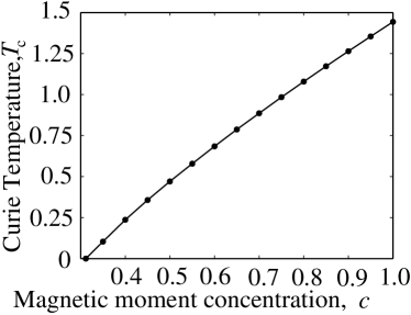
Figure 1: Curie temperatures calculated from Monte Carlo (filled circles) for a range of disorder strengths from the pure case $c=1$ to the site percolation threshold where $c=0.3116$.

concentration	$T_{c}$ (units of $J_{0}/k_{\mathrm{B}}$)	$K_{c}$ (units of $k_{\mathrm{B}}/J_{0}$)
$c=1.0$	1.4430	0.6930
$c=0.95$	1.3543	0.7384
$c=0.90$	1.2641	0.7911
$c=0.80$	1.0787	0.92705
$c=0.70$	0.88590	1.1288
$c=0.60$	0.6840	1.462
$c=0.50$	0.4701	2.127
$c=0.40$	0.2361	4.235

Table 1: $T_{c}$ values (with the uncertainty in the last digit for each concentration $c$ given). The $T_{c}$ results are given in units of $J_{0}/k_{\mathrm{B}}$, whereas the inverse temperatures $K_{c}$ are expressed in terms of $k_{\mathrm{B}}/J_{0}$.

The calculation of critical exponents involves the exploitation of finite size scaling trends easily obscured by statistical fluctuations stemming from the random character of the disorder, and hence it is necessary to average over many realizations of disorder, $10^{5}$ for $c<0.9$, and at least $4\times 10^{4}$ for weak disorder where $c=0.9$ and $c=0.95$, as well as the pure case where $c=1.0$. The large-scale Monte Carlos calculations have a significant parallel element, and we have benefited from the use of the HPCC (High Performance Computing Cluster) at the University of Maryland, cumulatively using approximately a CPU decade to complete the calculations we report on here.

To circumvent critical slowing down plaguing local update techniques such as the Metropolis method, our Monte-Carlo calculations employ cluster updates to flip large sets of correlated spins. Specifically, we use alternating Wolff cluster Wolff and Swendsen-Wang sweeps Swend , the latter being included because the Swendsen-Wang steps ultimately flip every spin, including isolated clusters of moments inaccessible to Wolff cluster moves. The cluster moves operate by flipping groups of thermodynamically correlated spins, and are effective even in the vicinity of $T_{c}$ where the diverging correlation length $\xi$ would otherwise be associated with a much larger Monte-Carlo autocorrelation time, as certainly would be encountered with the use of the Metropolis method.

To reduce the severity of finite size effects, we examine cubic systems of size $L$ with periodic boundary conditions. We use 1000 hybrid sweeps per disorder realization, and equilibration effects are eliminated by discarding the first quarter of the Monte Carlo sweeps. Monte Carlo calculations require stochastic input, and we use a Mersenne Twister algorithm to minimize correlations among random numbers and to ensure the period of the sequence far exceeds the number of random numbers used over the span of the Monte Carlo simulations.

Thermal derivatives such as $d\xi/dT$ need not be calculated via numerical differentiation; it is more convenient instead to use $d\langle g\rangle/dT=(\langle qE\rangle-\langle q\rangle\langle E\rangle)/(k_{\textrm{B}}T)$ obtained by direct differentiation of $\langle q\rangle=\sum_{\mathrm{conf}}q_{\mathrm{conf}}\exp(-E_{\mathrm{conf}}/k_{\mathrm{B}}T)/Z$, where the sum is over all possible system configurations, $Z$ is the partition function, $E$ is the internal energy, and $q$ is a generic thermodynamic variable such as the magnetization.

By examining the parameter $g_{2}$, which provides a measure of typical fluctuations from one realization of disorder to the next, we find clear evidence of self-averaging at the critical temperature $T_{c}$. Results for $g_{2}$ for a range of disorder strengths are shown in Fig. 2. The $\log$-$\log$ $g_{2}$ curves are non-monotonic, increasing for small values of $L$ and attaining a maximum (typically for systems containing on the order of 700 spins) before decreasing and ultimately becoming linear for sufficiently small system sizes. An asymptotic power law decay in $L$ of $g_{2}$ for large system sizes is consistent with a monotonic decreases of $g_{2}$, a hallmark of self-averaging in the bulk limit.

A more subtle question is whether disorder has an effect on the critical behavior of the Heisenberg model. Asymptotic finite size scaling behavior such as $m\propto L^{-\beta/\nu}$, $\chi\propto\chi_{0}L^{\gamma/\nu}$, and $d\xi/dT\propto L^{1/\nu}$ imply the corresponding $\log-\log$ plots will become linear for large enough $L$ with the slope yielding the critical exponent of interest. However, although singular thermodynamic quantities such as the magnetization $m$ and the susceptibility $\chi$ vary asymptotically as $\chi=\chi_{0}L^{\gamma/\nu}$ and $m=m_{0}L^{-\beta/\nu}$, respectively, site disorder is a source of important corrections to leading order scaling, which must be taken into account to obtain accurate expressions for critical exponents such as $\gamma/\nu$ and $\beta/\nu$. Hence, in addition to the amplitude and exponent of the most singular contributions to $\chi$ and $m$, we perform nonlinear least squares fitting to take into account the next-to leading order exponent and amplitude relative to that of the leading term with

$$\chi(L)=\chi_{0}(L^{\gamma/\nu}+B_{\gamma}L^{\epsilon_{\gamma}});$$ (1)

$$m(L)=m_{0}(L^{-\beta/\nu}+B_{\beta}L^{\epsilon_{\beta}});$$ (2)

$$\frac{d\xi}{dT}(L)=A_{\nu}^{0}(L^{1/\nu}+B_{\nu}L^{\epsilon_{\nu}}),$$ (3)

where the coefficients $B$ are the relative amplitude of the first correction to primary scaling, and the exponents labeled $\epsilon$ are next to leading order exponents.

We calculate critical exponents and amplitudes by minimizing the sum of the squares of the relative differences, e.g. for the magnetic susceptibility exponent $\gamma$, with $\sigma=\tfrac{1}{N}\left[\displaystyle{\sum_{i=1}^{N}}\left(\tfrac{\gamma_{L_{i}}^{\mathrm{MC}}-\gamma_{L_{i}}^{\mathrm{LSF}}}{\gamma_{L_{i}}^{\mathrm{MC}}}\right)^{2}\right]^{1/2}$, where $\gamma_{L_{i}}$ is calculated numerically with Monte Carlo simulations and $\gamma_{L_{i}}^{\mathrm{LSF}}$ is given in Eq. 1 for the system size $L_{i}$. To carry out the nonlinear least squares fitting, we use a stochastic algorithm with an annealing stage (i.e. the Metropolis Criterion is used with the quantity $\sigma$ treated as an “energy” and the “temperature” reduced at a linear rate in the number of Monte Carlo sweeps over the exponents and amplitudes) to minimize $\sigma$ by randomly perturbing exponents and amplitudes; after the annealing phase, the Monte Carlo moves in the exponent and amplitude space are accepted only if the sum of the squares of differences is thereby reduced. To navigate the shallow “energy” landscape corresponding to $\sigma$, the average magnitude of the random shifts is augmented (decreased) by a factor $(1+\epsilon)$ if a move is accepted (rejected) with $\epsilon\sim 10^{-5}$. In addition, we check for convergence of the critical exponents and amplitudes by successively doubling the time span of the annealing until the results cease to change.

In experiment, the reduced temperature $t$ is more readily tuned than the system size. To show how the effective critical behavior may vary appreciably for, we calculate the magnetic susceptibility $\chi$ for $t>0$, but in the bulk limit as would be appropriate for comparison experiment. For finite $t$, it is sufficient to examine system sizes, such that $L\gg\xi$ since the correlation length will be finite for temperatures above $T_{c}$. We find the condition $\xi/L<0.06$ is sufficient to reduce finite size to a negligible level. In addition, by calculating $\chi$ for a number of different system sizes, we may correct for finite size effects; we have explicitly verified that a relation of the form $A+Be^{-\kappa L/xi}$ is a very good approximation to the dependence of thermodynamic variable on system size when $L$ is at least on the order of a few correlation lengths, a condition we use to further improve our approximation to bulk behavior, or to relax somewhat the condition $\xi/L<0.06$ by examining somewhat smaller systems and subsequently removing residual finite size effects.

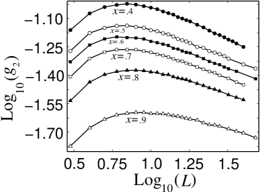
Figure 2: The graph contains $\log$-$\log$ traces of the self-averaging parameter $g_{2}=[\langle m^{2}\rangle^{2}]-[\langle m^{2}\rangle]^{2}$ for the second moment of the magnetization for very weak ($c=0.95$) to quite strong disorder ($c=0.40$); symbols are from Monte-Carlo calculations, and the solid line is a guide to the eye.

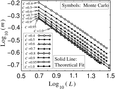
Figure 3: The image shows $\log$-$\log$ plots of the magnetization $m$ versus system size $L$ for the pure Heisenberg model where $c=1.0$, and disorder ranging from quite weak ($c=0.95$) to very strong ($c=0.40$). The symbols are results from Monte Carlo calculations, and the solid lines are theoretical fits.

Figure 4: The graph contains $\log$-$\log$ plots of the magnetic susceptibility $\xi$ versus $L$ for the pure Heisenberg model with $c=1.0$, and disorder ranging from quite weak ($c=0.95$) to very strong ($c=0.40$). The symbols are results from Monte Carlo calculations, and the solid lines are theoretical fits.

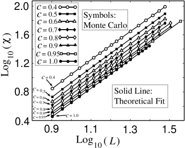
Figure 5: Shown are $\log$-$\log$ traces of the thermal derivative of the correlation length $d\xi/dT$ versus $L$ for the pure Heisenberg model ($c=1.0$), and magnetic moment concentrations ranging from very weak ($c=0.95$) to quite strong disorder ($c=0.40$). Symbols are Monte Carlo data, and the solid lines are theoretical fits.

concentration $c$	$\beta_{\mathrm{pure}}/\nu_{\mathrm{pure}}$	$\beta/\nu$	$m_{0}$	$\epsilon_{\beta}$	$B_{\beta}$
$c=1.0$	0.516	0.5159	1.083	-2.365	-0.233
$c=0.95$	0.516	0.5150	1.096	-2.242	-0.2269
$c=0.90$	0.516	0.5143	1.114	-1.975	-0.2001
$c=0.80$	0.516	0.5080	1.142	-2.038	-0.2538
$c=0.7$	0.516	0.5106	1.221	-1.648	-0.2651
$c=0.6$	0.516	0.5248	1.386	-1.305	-0.3164
$c=0.5$	0.516	0.5233	1.485	-1.373	-0.3779
$c=0.4$	0.516	0.5011	1.498	-1.919	-0.5600

Table 2: Critical exponent ratios $\beta/\nu$ for the magnetization with the amplitude $m_{0}$ of the leading order term, the exponent $\epsilon_{\beta}$ of the first correction to primary scaling, and the relative amplitude $B_{\beta}$ of the next-to leading order term.

concentration $c$	$\gamma_{\mathrm{pure}}/\nu_{\mathrm{pure}}$	$\gamma$	$\chi_{0}$	$\epsilon_{\gamma}$	$B_{\gamma}$
$c=1.0$	1.955	1.957	0.05206	0.9468	-0.5276
$c=0.95$	1.955	1.963	0.05426	0.2783	-1.309
$c=0.90$	1.955	1.954	0.0598	0.4372	-1.054
$c=0.80$	1.955	1.935	0.0724	0.9121	-0.6482
$c=0.70$	1.955	1.973	0.07037	-0.7585	-7.574
$c=0.60$	1.955	1.977	0.08014	0.2133	-1.957
$c=0.50$	1.955	1.993	0.08915	-0.8402	-15.86
$c=0.40$	1.955	1.945	0.1317	-0.7112	-15.91

Table 3: Critical exponent ratios $\gamma/\nu$ for the magnetization with the amplitude $\chi_{0}$ of the leading order term, the exponent $\epsilon_{\gamma}$ of the first correction to primary scaling, and the relative amplitude $B_{\gamma}$ of the next-to leading order term.

concentration $c$	$\eta_{\mathrm{pure}}$	$\eta$
$c=1.0$	0.038	0.043
$c=0.95$	0.038	0.037
$c=0.90$	0.038	0.046
$c=0.80$	0.038	0.065
$c=0.70$	0.038	0.027
$c=0.60$	0.038	0.023
$c=0.50$	0.038	0.007
$c=0.40$	0.038	0.046

Table 4: Critical exponents $\eta$ for disorder ranging from the pure case ($c=1.0$) to strong disorder where $c=0.4$.

concentration $c$	$\nu_{\mathrm{pure}}$	$\nu$	$A_{\nu}^{0}$	$\epsilon_{\nu}$	$r_{\nu}$
$c=1.0$	0.714	0.7149	0.2862	-1.428	2.798
$c=0.95$	0.714	0.7291	0.2500	-1.2543	1.760
$c=0.9$	0.714	0.7335	0.2045	0.4941	0.2366
$c=0.80$	0.714	0.7412	0.1322	0.7347	0.3706
$c=0.70$	0.714	0.7428	0.07814	0.7675	0.5878
$c=0.60$	0.714	0.7018	0.02545	0.9572	1.923
$c=0.50$	0.714	0.7188	0.01330	0.8838	1.759
$c=0.40$	0.714	0.6997	0.00261	0.6612	4.485

Table 5: Correlation length critical exponents $\nu$ for $d\xi/dT$ with the amplitude $A_{\nu}^{0}$ of the leading order term, the exponent $\epsilon_{\nu}$ of the first correction to scaling, and the relative amplitude $r_{\nu}$ of the first correction term.

III Critical Behavior of the Disordered Heisenberg Model

The $\log$-$\log$ plots in Fig. 3 show the magnetization with symbols representing Monte Carlo results, and the continuous curves are obtained from the corresponding nonlinear least squares fits. The excellent agreement of the Monte Carlo data and theoretical fits may also be seen in the Appendix, where the simulation data and theoretical results are given to five significant figures. Similarly, the magnetic susceptibilities appear in Fig. 4, where symbols represent the Monte Carlo results and solid lines obtained from theoretical fits closely match the Monte Carlo data. Finally, the correlation length thermal derivatives $d\xi/dT$ are graphed in Fig. 5, and there is again good agreement between Monte Carlo results (symbols) and the solid lines obtained from theoretical results.

Exponents and critical amplitudes are given for $\beta/\nu$ in Table 2, $\gamma/\nu$ (corresponding to the susceptibility) in Table 3, $\eta$ in Table 4, and $\nu$ in Table 5. The exponent $\eta$ is calculated from $\gamma$ and $\nu$ with $\eta=2\gamma/\nu$. The parameter $\eta$ is a sensitive parameter and, accordingly, there is greater variance in the results. However, the $\eta$ values listed in Table 4 each have the same positive sign irrespective of the strength of the site disorder. The leading order exponents are consistent with those of the pure Heisenberg Universality class with deviations due only to statistical Monte Carlo error, not systematic effects related to the disorder strength. Hence, since each of the exponents $\beta$, $\nu$, $\gamma$, and $\eta$ are stable with respect to the introduction of site defects, we conclude for the Heisenberg model that critical behavior is unchanged even in the presence of very strong disorder.

IV Effective Critical Behavior and Apparent Violation of the Harris Criterion

Although ultimately we find that the critical behavior of the pure Heisenberg model emerges as the dominant part of the singular components of thermodynamic variables such as the magnetization $m$ and magnetic susceptibility $\chi$, finite size effects may obscure the genuine critical behavior for systems of small to moderate size where bulk critical behavior has not taken hold. Fig. 6, Fig. 7, and Fig. 8 show the apparent critical indices which would be obtained as the slope $d\log(\chi)/d\log(t)=\tfrac{t}{\chi}\tfrac{d\chi}{dt}$ of the log-log graph, a quantity which may differ significantly for the first several decades of the system size $L$ before eventually converging to the critical indices of the pure Heisenberg model, indicated with horizontal gray lines. Qualitatively similar behavior has been seen in renormalization group (RG) calculations Dudka as well as in experiment Fahnle ; Kaul1 ; Kaul2 ; Kaul3 ; Babu ; Perumal with the reduced temperature $t$ varied instead of the system size $L$. The insets of Fig. 6, Fig. 7, and Fig. 8 display $\beta/\nu$, $\gamma/\nu$, and $\nu$ obtained from the nonlinear least squares fits. Again, throughout the broad disorder spectrum considered, even for very strongly strongly disordered systems (e.g. for the case $c=0.4$), the critical indices we calculate are compatible with those of the pure system where there is no disorder.

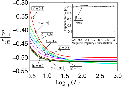
Figure 6: (color online) Effective $\beta/\nu$ curves are shown in a semi-logarithmic graph for various impurity concentrations $c$ for several decades of $L$. The inset shows the calculated $\beta/\nu$ values versus the impurity concentration. The horizontal gray lines in both the primary graph and the inset correspond to $\beta/\nu$ for the pure system.

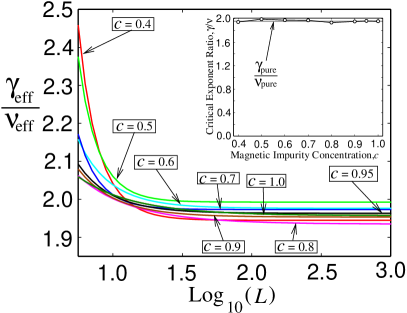
Figure 7: (color online) Effective $\gamma/\nu$ curves are graphed in a semi-logarithmic plot for various impurity concentrations $c$ for several decades of system sizes, with the inset showing $\gamma/\nu$ versus the impurity concentration $c$. The horizontal gray lines in the main figure and graph inset indicate $\gamma_{\mathrm{pure}}/\nu_{\mathrm{pure}}$ for the case where there is no disorder.

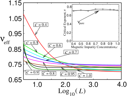
Figure 8: (color online) Effective $\nu$ curves are plotted in a semi-logarithmic fashion for a range of magnetic moment concentrations $c$ for a few decades of $L$; the inset is a graph of the calculated exponent $\nu$ versus $c$. Again, the horizontal gray lines correspond to $\nu_{\mathrm{pure}}$ for the case $c=1$.

To make direct contact with experiment and show explicitly the apparent change in critical behavior may be set up by strong disorder, we show finite $t$ results where the effective critical exponent $\gamma_{\mathrm{eff}}$ corresponding to the magnetic susceptibility has been calculated; results are shown in panel (a) and panel (b) of Fig. 9. For $t>0$, the susceptibility $\chi$ will scale as $\chi=\chi_{0}(t^{-\gamma}+Bt^{y_{1}}+Ct^{y_{2}}+Dt^{y_{3}}+\ldots)$ where $\gamma$ is the genuine critical exponent for $\chi$, and the terms with exponents such as $y_{1}$, $y_{2}$ for the first two subleading terms are corrections to scaling which may have a significant effect if $t$ is sufficiently large or in the presence of strong enough disorder.

In the critical regime where subleading terms may be neglected, one may compute, e.g. for $\chi$, $\gamma=-\tfrac{t}{\chi}d\chi/dt$. However, further from $T_{c}$ where corrections to singular critical behavior are more important, one obtains an “effective” exponent $\gamma(t)$ given by

$$\gamma(t)\equiv\frac{-t}{\chi}\frac{d\chi}{dt}=\gamma\left(\frac{1+By_{1}t^{y_{1}+\gamma}+Cy_{2}t^{y_{2}+\gamma}+\ldots}{1+Bt^{y_{1}+\gamma}+Ct^{y_{2}+\gamma}+\ldots}\right);$$ (4)

$\gamma(t)$ will eventually tend to the leading order exponent $\gamma$ as $t\rightarrow 0$, though one may have to measure $\chi$ at very low values of $t$ if there is a strong disorder component.

The graphs shown in Fig. 9 show results from two distinct calculations of $\gamma(t)$. In panel (a) of Fig. 9, the Monte Carlo data is drawn from a study where fewer disorder realizations are examined (though still at least $5\times 10^{3}$ configurations of disorder are analyzed) in favor of obtaining a larger data set; Monte Carlo results are shown as symbols with theoretical curves obtained from nonlinear least square fitting shown on the same graph. Similarly, for the set of calculations involving fewer data points but more intensive disorder averaging, Monte Carlo data is graphed as symbols in panel (b) of Fig. 9, while again solid lines are theoretical curves gleaned from least squares fitting.

In both cases, although $\gamma(t)$ for the pure $(c=1)$ case rises steadily with decreasing $t$, the curves for each of the disordered systems are nonmonotonic; the initial rise with decreasing $t$ is followed by a peak and subsequent decline to the asymptotic value of $\gamma$ only for very small values of the reduced temperature on the order of $t\sim 10^{-3}$.

We reiterate that the critical exponents we calculate are consistent with $\nu>2/3$ where disorder is irrelevant to the universality class in the Renormalization Group (RG) sense This inequality has been placed on a rigorous footing in theoretical work Chayes under a broad range of conditions, and has also been established for correlated disorder Weinrib . We also emphasize that while the genuine Heisenberg model critical exponents satisfy the hyperscaling relations, the apparent critical exponents obtained away from the critical behavior are not consistent with the hyperscaling formulas, an indication of their problematic nature.

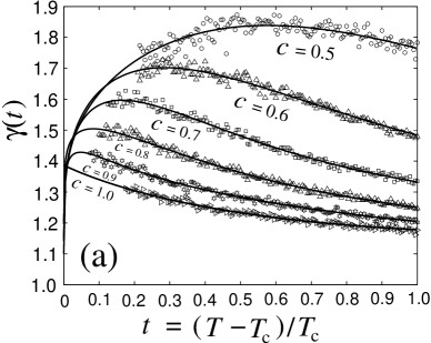
Figure 9: Panel (a) shows the effective magnetic susceptibility exponent $\gamma(t)$ versus the reduced temperature $t$. The solid curves are analytical results from the least square fitting, and the symbols represent Monte Carlo data. In panel (b), solid curves are again obtained from least squares fitting, and the symbols are Monte Carlo data.

V Conclusions

In conclusion, within a large-scale Monte Carlo study, we have examined Heisenberg models on three dimensional lattices with randomly deleted magnetic moments as a source of disorder, finding self-averaging to be intact as predicted by the Harris criterion. Moreover, our finite size scaling studies show leading order critical behavior not to be influenced by the presence of random defects, with critical exponents identical to those of the pure Heisenberg model universality class even for very strong disorder in the vicinity of the site percolation threshold where long-range ferromagnetic order is lost altogether for $T<0$. However, while the leading order exponents are not sensitive to disorder, the presence of site defects sets up corrections to primary scaling which skew the effective exponents for finite system sizes $L$, a characteristic which might naïvely be regarded as evidence for the violation of the Harris criterion. A qualitatively similar apparent violation of the Harris criterion is seen in experiment where thermodynamic quantities such as the magnetic susceptibility are measured with respect to the reduced temperature $t$, and we have also calculate the same quantities in the bulk limit for $t>0$, finding the same apparent violation of the Harris criterion. We conclude by asserting the asymptotic validity of the Harris criterion sufficiently close to the critical temperature in the strongly disordered Heisenberg model appropriate for diluted magnetic semiconductors, at the same time pointing out that slightly away from the critical temperature, the effective exponents may very well reflect an apparent (and incorrect) violation unless extremely careful measures are taken to include finite-size scaling and corrections to scaling in the analyses

VI Appendix: Thermodynamic Quantities from Monte Carlo and Analytical Fits

The appendix contains a sequence of tables explicitly giving thermodynamic quantities calculated in Monte Carlo simulations with the theoretical fits obtained by stochastically enhanced least squares fitting. The theoretical results are in very close agreement with the corresponding Monte Carlo data.

$n$	$m^{x=1.0}_{\mathrm{num}}$	$m^{x=1.0}_{\mathrm{fit}}$	$\chi^{x=1.0}_{\mathrm{num}}$	$\chi^{x=1.0}_{\mathrm{fit}}$	$\frac{d\xi}{dT}^{x=1.0}_{\mathrm{num}}$	$\frac{d\xi}{dT}^{x=1.0}_{\mathrm{fit}}$
$5$	0.46661	0.46662
$6$	0.42624	0.42620
$7$	0.39444	0.39445
$8$	0.36869	0.36871	2.8510	2.8512	5.2874	5.2882
$9$	0.34730	0.34731	3.6186	3.6181	6.2244	6.2216
$10$	0.32915	0.32917	4.4759	4.4740	7.2043	7.1992
$11$	0.31357	0.31355	5.4184	5.4148	8.2064	8.2178
$12$	0.29991	0.29991	6.4509	6.4481	9.2678	9.2749
$13$	0.28786	0.28787	7.5750	7.5712	10.372	10.369
$14$	0.27717	0.27714	8.7794	8.7790	11.495	11.497
$15$	0.26754	0.26751	10.075	10.074	12.677	12.658
$16$	0.25880	0.25879	11.460	11.456	13.853	13.851
$17$	0.25084	0.25086	12.924	12.924	15.065	15.074
$18$	0.24358	0.24360	14.480	14.480	16.331	16.326
$19$	0.23690	0.23693	16.120	16.121	17.618	17.607
$20$	0.23077	0.23076	17.844	17.848	18.906	18.915
$22$	0.21972	0.21972	21.547	21.560	21.586	21.609
$23$	0.214763	0.21475	23.559	23.545	22.996	22.994
$24$	0.21013	0.21010	25.609	25.614	24.391	24.403
$25$	0.20573	0.20573	27.774	27.769	25.859	25.836

Table 6: Thermodynamic quantities from Monte Carlo simulations and theoretical fits for the pure system, where $c=1.0$.

$n$	$m^{x=0.95}_{\mathrm{num}}$	$m^{x=0.95}_{\mathrm{fit}}$	$\chi^{x=0.95}_{\mathrm{num}}$	$\chi^{x=0.95}_{\mathrm{fit}}$	$\frac{d\xi}{dT}^{x=0.95}_{\mathrm{num}}$	$\frac{d\xi}{dT}^{x=0.95}_{\mathrm{fit}}$
$5$	0.47156	0.47162
$6$	0.43115	0.43101
$7$	0.39900	0.39908
$8$	-.37323	0.37317	3.0920	3.0911	4.3618	4.3626
$9$	0.35155	0.35161	3.9221	3.9241	5.1192	5.1173
$10$	0.33341	0.33332	4.8492	4.8521	5.9058	5.9050
$11$	0.31749	0.31756	5.8821	5.8747	6.7220	6.7234
$12$	0.30387	0.30380	6.9917	6.9915	7.5733	7.5706
$13$	0.29147	0.29165	8.2009	8.2022	8.4337	8.4448
$14$	0.28075	0.28082	9.4934	9.5065
$15$	0.27108	0.27109	10.912	10.904	10.278	10.269
$16$	0.26227	0.26228	12.396	12.395	11.216	11.217
$17$	0.25435	0.25427	13.983	13.978	12.173	12.188
$18$	0.24699	0.24693	15.666	15.655	13.197	13.179
$20$	0.23401	0.23395	19.286	19.284	15.242	15.225
$22$	0.22290	0.22279	23.237	23.281	17.323	17.349
$24$	0.21295	0.21306	27.658	27.646	19.546	19.545
$26$	0.20443	0.20448	32.391	32.376	21.816	21.811
$36$			61.475	61.475

Table 7: Monte-Carlo results and theoretical fits for thermodynamic quantities for a weakly disordered Heisenberg model with $c=0.95$.

$n$	$m^{x=0.9}_{\mathrm{num}}$	$m^{x=0.9}_{\mathrm{fit}}$	$\chi^{x=0.9}_{\mathrm{num}}$	$\chi^{x=0.9}_{\mathrm{fit}}$	$\frac{d\xi}{dT}^{x=0.9}_{\mathrm{num}}$	$\frac{d\xi}{dT}^{x=0.9}_{\mathrm{fit}}$
$5$	0.47733	0.47747
$6$	0.43701	0.43671
$7$	0.40455	0.40463
$8$	0.37850	0.37856	3.3201	3.3184	2.4417	2.4127
$9$	0.35689	0.35685	4.2089	4.2092	2.8128	2.8098
$10$	0.33837	0.33842	5.1921	5.2010	3.2218	3.2212
$11$	0.32250	0.32253	6.2947	6.2933	3.6437	3.6461
$12$	0.30863	0.30863	7.4897	7.4857	4.0835	4.0835
$13$	0.29638	0.29636	8.7799	8.7776	4.5272	4.5330
$14$	0.28531	0.28541	10.1715	10.1687	4.9940	4.9938
$15$	0.27551	0.27558	11.670	11.659	5.4648	5.4655
$16$	0.26670	0.26667	13.245	13.247	5.9519	5.9475
$17$	0.25862	0.25856	14.928	14.933	6.4421	6.4396
$18$	0.25126	0.25113	16.714	16.718	6.9451	6.9412
$20$	0.23784	0.23799	20.604	20.579	7.9753	7.9719
$22$	0.22676	0.22668	24.797	24.828	9.0375	9.0373
$24$	0.21689	0.21681	29.428	29.464	10.136	10.135
$26$	0.20809	0.20811	34.484	34.484	11.253	11.264
$28$	0.20038	0.20036	39.888	39.906	12.411	12.422
$32$	0.18796	0.18712	51.840	51.863	14.835	14.821

Table 8: Monte Carlo data and corresponding theoretical fits for the magnetization, magnetic susceptibility, and $d\xi/dT$ for mildly disordered Heisenberg models ($c=0.9$).

$n$	$m^{x=0.8}_{\mathrm{num}}$	$m^{x=0.8}_{\mathrm{fit}}$	$\chi^{x=0.8}_{\mathrm{num}}$	$\chi^{x=0.8}_{\mathrm{fit}}$	$\frac{d\xi}{dT}^{x=0.8}_{\mathrm{num}}$	$\frac{d\xi}{dT}^{x=0.8}_{\mathrm{fit}}$
$5$	0.49310	0.49316
$6$	0.45209	0.45195
$7$	0.41946	0.41937
$8$	0.39240	0.39282	3.7346	3.7337	2.4117	2.4127
$9$	0.37079	0.37065	4.7334	4.7340	2.8128	2.8098
$10$	0.35190	0.35180	5.8429	5.8480	3.2218	3.2212
$11$	0.33547	0.33552	7.0858	7.0751	3.6437	3.6461
$12$	0.32145	0.32127	8.4009	8.4145	4.0835	4.0835
$13$	0.30867	0.30867	9.8800	9.8655	4.5272	4.5330
$14$	0.29742	0.29743	11.417	11.427	4.9940	4.9938
$15$	0.28726	0.28731	13.090	13.100	6.4421	6.4396
$16$	0.27804	0.27815	14.888	14.882	5.9519	5.9475
$17$	0.26980	0.26981	16.799	16.774	6.4421	6.4396
$18$	0.26212	0.26216	18.776	18.775	6.9451	6.9412
$20$	0.24868	0.24861	23.101	23.103	7.9753	7.9719
$22$	0.23693	0.23694	27.865	27.862	9.0375	9.0373
$24$	0.22681	0.22676	33.003	33.050	10.136	10.135
$26$	0.21781	0.21777	38.657	38.664	11.253	11.264
$28$	0.20973	0.20977	44.733	44.702	12.411	12.422
$32$	0.19605	0.19607	58.050	58.043	14.835	14.821

Table 9: Monte Carlo results with theoretical fits for key thermodynamic quantities in the case of moderate disorder, where $c=0.8$.

$n$	$m^{x=0.7}_{\mathrm{num}}$	$m^{x=0.7}_{\mathrm{fit}}$	$\chi^{x=0.7}_{\mathrm{num}}$	$\chi^{x=0.7}_{\mathrm{fit}}$	$\frac{d\xi}{dT}^{x=0.7}_{\mathrm{num}}$	$\frac{d\xi}{dT}^{x=0.7}_{\mathrm{fit}}$
$5$	0.51371	0.51391
$6$	0.47241	0.47211
$7$	0.4389	0.43889
$8$	0.41201	0.41168	4.1464	4.1492	1.5110	1.5109
$9$	0.38852	0.38890	5.2738	5.2730	1.7535	1.7530
$10$	0.36941	0.36945	6.5313	6.5225	2.0032	2.0033
$11$	0.35261	0.35261	7.8917	7.8978	2.2611	2.2611
$12$	0.33768	0.33785	9.4050	9.3988	2.5235	2.5262
$13$	0.32469	0.32477	11.033	11.026	2.7974	2.7980
$14$	0.31308	0.31308	12.779	12.778	3.0780	3.0763
$15$	0.30259	0.30254	14.642	14.655	3.3598	3.3608
$16$	0.29296	0.29299	16.661	16.658	3.6553	3.6512
$17$	0.28451	0.28428	18.756	18.786	3.9476	9.9472
$18$	0.27625	0.27629	21.043	21.039	4.2492	4.2487
$20$	0.26210	0.26211	25.936	25.919	4.8674	4.8675
$22$	0.24997	0.24989	31.328	31.298	5.5083	5.5059
$24$	0.23933	0.23921	37.109	37.173	6.1555	6.1630
$26$	0.22973	0.22977	43.532	43.544	6.8363	6.8376
$28$	0.22125	0.22135	50.435	50.410	7.5259	7.5290
$30$	0.21377	0.21379	57.808	57.770	8.2433	8.2364

Table 10: Monte Carlo results and theoretical fits for thermodynamic quantities corresponding to critical exponents $\beta$, $\gamma$, and $\nu$ for a range of system sizes $L$ for moderate disorder $c=0.7$.

$n$	$m^{x=0.6}_{\mathrm{num}}$	$m^{x=0.6}_{\mathrm{fit}}$	$\chi^{x=0.6}_{\mathrm{num}}$	$\chi^{x=0.6}_{\mathrm{fit}}$	$\frac{d\xi}{dT}^{x=0.6}_{\mathrm{num}}$	$\frac{d\xi}{dT}^{x=0.6}_{\mathrm{fit}}$
$5$	0.54158	0.54165
$6$	0.49865	0.49869
$7$	0.464646	0.464353
$8$	0.43616	0.43612	4.6385	4.6408	0.85119	0.85087
$9$	0.41211	0.41237	5.9258	5.9152	0.98288	98364
$10$	0.39194	0.39205	7.3248	7.3370	1.1209	1.1206
$11$	0.37460	0.37440	8.9036	8.9058	1.2616	1.2614
$12$	0.35895	0.35889	10.622	10.621	1.4060	1.4060
$13$	0.34494	0.34512	12.513	12.483	1.5528	1.5541
$14$	0.33278	33279	14.457	14.491	1.7085	1.7056
$15$	0.32167	0.32166	16.652	16.644	1.8594	1.8604
$16$	0.31144	0.31156	18.917	18.942	2.0172	2.0183
$17$	0.30233	0.30240	21.374	21.386	2.1776	2.1792
$18$	0.293935	0.293852	24.026	23.975	2.3468	2.3430
$20$	0.278766	0.27880	29.614	29.586	2.6786	2.6790
$22$	0.26589	0.26579	35.780	35.775	3.0249	3.0257
$24$	0.25447	0.25442	42.481	421.540	3.3835	3.3825
$26$	0.24429	0.24435	49.879	49.833	3.7460	3.7490
$28$	0.23538	0.23537	57.848	57.792	4.1222	4.1246
$30$	0.22724	0.22729	66.285	66.278	4.5131	4.5091

Table 11: Monte Carlo and corresponding theoretical fits for $m$, $\xi$, and $d\xi/dT$ for moderate disorder with $c=0.6$.

$n$	$m^{x=0.5}_{\mathrm{num}}$	$m^{x=0.5}_{\mathrm{fit}}$	$\chi^{x=0.5}_{\mathrm{num}}$	$\chi^{x=0.5}_{\mathrm{fit}}$	$\frac{d\xi}{dT}^{x=0.5}_{\mathrm{num}}$	$\frac{d\xi}{dT}^{x=0.5}_{\mathrm{fit}}$
$5$	0.57792	0.57819
$6$	0.53377	0.53361
$7$	0.49814	0.49769
$8$	0.46811	0.46798	5.3682	5.3740	0.38645	0.38685
$9$	0.44278	0.44290	6.8930	6.8840	0.44592	0.44569
$10$	0.42123	0.42136	8.5446	8.5634	0.50648	0.50621
$11$	0.40260	0.40262	10.433	10.413	0.56934	0.56834
$12$	0.38581	0.38612	12.436	12.433	0.63200	0.63198
$13$	0.37120	0.37145	14.682	14.625	0.69651	0.69706
$14$	0.35809	0.38612	17.011	16.989	0.76389	0.76352
$15$	0.34653	0.34641	19.477	19.524	0.82997	0.83131
$16$	0.33573	0.33561	22.203	22.231	0.89980	0.90038
$17$	0.32568	0.32573	25.120	25.111	0.97058	0.97067
$18$	0.31677	0.31666	28.156	28.162	1.0406	1.0422
$20$	0.28662	0.28659	34.610	34.781	1.1904	1.1885
$22$	0.28662	0.28659	42.166	42.089	1.3404	1.3392
$24$	0.27434	0.27438	50.003	50.085	1.4937	1.4940
$26$	0.263647	0.263579	58.783	58.769	1.6535	1.6528
$28$	0.25390	0.25393	68.260	68.142	1.8176	1.8152
$30$	0.24509	0.24525	78.284	78.203	1.9782	1.9812

Table 12: Thermodynamic quantities from Monte Carlo simulations and corresponding theoretical fits for strong disorder with half of the magnetic moments missing, $c=0.5$.

$n$	$m^{x=0.4}_{\mathrm{num}}$	$m^{x=0.4}_{\mathrm{fit}}$	$\chi^{x=0.4}_{\mathrm{num}}$	$\chi^{x=0.4}_{\mathrm{fit}}$	$\frac{d\xi}{dT}^{x=0.4}_{\mathrm{num}}$	$\frac{d\xi}{dT}^{x=0.4}_{\mathrm{fit}}$
$5$	0.63025	0.63036
$6$	0.58355	0.58327
$7$	0.54462	0.54481
$8$	0.51280	0.51278	7.0363	7.0359	0.097086	0.09711
$9$	0.48570	0.48564	9.0001	9.0083	0.11011	0.11018
$10$	0.46236	0.46230	11.189	11.188	0.12359	0.12358
$11$	0.44190	0.44195	13.601	13.577	0.13720	0.13728
$12$	0.42378	0.42403	16.158	16.173	0.15144	0.15128
$14$	0.39391	0.39381	22.029	21.989	0.18022	0.18016
$15$	0.38075	0.38091	25.166	25.208	0.19493	0.19501
$16$	0.36932	0.36918	28.596	28.634	0.20974	0.21014
$17$	0.35837	0.35846	32.245	32.265	0.22537	0.22554
$18$	0.34866	0.34861	36.164	36.103	0.24193	0.24119
$20$	0.33109	0.33112	44.376	44.394	0.27323	0.27325
$22$	0.31595	0.31600	53.543	53.501	0.30523	0.30627
$24$	0.30289	0.30277	63.347	63.423	0.33949	0.34023
$26$	0.29122	0.29106	73.934	74.155	0.37480	0.37508
$28$	0.28050	0.28060	85.867	85.693	0.41256	0.41079
$30$	0.27112	0.27119	98.147	98.036	0.44716	0.44733

Table 13: Monte Carlo data and theoretical fits for the magnetization, susceptibility, and $d\xi/dT$ for the case $c=0.4$ of very strong disorder in the vicinity of the site percolation threshold, $c=0.3116$.

Table 14 and Table 15 contain the self-averaging parameter $g_{2}$ for various systems sizes for site disorder ranging from the weak regime (where $c=0.95$), to the strongly disordered $c=0.40$ case in the vicinity of the percolation threshold. A consistent feature in the dependence of $g_{2}$ on system size is an initial rise, and maximum attained for moderate sized systems with on the order of 700 spins. After reaching a peak, the $g_{2}$ self-averaging parameter begins a steady decrease consistent with intact self-averaging. However, the non-monotonic behavior is another manifestation of significant corrections to leading order scaling.

$n$	$g_{2}^{x=0.95}$	$g_{2}^{x=0.90}$	$g_{2}^{x=0.80}$	$g_{2}^{x=0.70}$
$4$	0.011629	0.021031	0.036693	0.048896
$5$	0.012967	0.023353	0.040195	0.052853
$6$	0.013691	0.024601	0.041686	0.054397
$7$	0.013910	0.025078	0.042294	0.054408
$8$	0.014214	0.025350	0.042353	0.054383
$9$	0.014231	0.025331	0.042114	0.053457
$10$	0.014260	0.024991	0.041469	0.052606
$11$	0.014404	0.025016	0.041237	0.051461
$12$	0.014242	0.024941	0.040218	0.050677
$13$	0.014139	0.024665	0.040141	0.049733
$14$	0.013823	0.024351	0.039113	0.048602
$15$	0.014003	0.024223	0.038562	0.047621
$16$	0.013857	0.023888	0.038132	0.047256
$17$	0.013882	0.023619	0.037801	0.046230
$18$	0.013685	0.023398	0.037099	0.045487
$20$	0.013441	0.023101	0.036060	0.044077
$22$	0.013139	0.022324	0.035145	0.042900
$24$	0.013017	0.021689	0.034176	0.041727
$26$	0.012982	0.021758	0.033564	0.041068
$28$		0.021433	0.032892	0.039746
$30$				0.039227
$32$		0.020729	0.031422	0.038045
$34$			0.037439
$36$	0.012127	0.020170	0.030430

Table 14: Values of the self-averaging parameter $g_{2}$ for weak to moderate disorder strengths.

$n$	$g_{2}^{x=0.6}$	$g_{2}^{x=0.5}$	$g_{2}^{x=0.40}$
$4$	0.057541	0.066634	0.091366
$5$	0.061999	0.070882	0.093814
$6$	0.063578	0.072695	0.095018
$7$	0.062970	0.072895	0.094071
$8$	0.062751	0.071787	0.092343
$9$	0.061942	0.070998	0.090638
$10$	0.060216	0.068958	0.089034
$11$	0.059253	0.068091	0.086531
$12$	0.058137	0.066394	0.084828
$13$	0.057270	0.065569	0.083349
$14$	0.055345	0.063845	0.080870
$15$	0.054770	0.061972	0.079409
$16$	0.053529	0.061077	0.077896
$17$	0.052644	0.060114	0.076659
$18$	0.052211	0.058970	0.073666
$20$	0.050329	0.056281	0.071286
$22$	0.048794	0.055587	0.068609
$24$	0.047155	0.053513	0.066323
$26$	0.046044	0.052511	0.064995
$28$	0.045294	0.051496	0.063222
$30$	0.044054	0.050261	0.061438
$32$	0.043114	0.048754	0.060254
$34$			0.058666
$36$	0.041824	0.056226

Table 15: Values of the self-averaging parameter $g_{2}$ for moderate to strong levels of disorder.

- (1) D. J. Priour and S. Das Sarma, Phys. Rev. Lett. 62, 127201 (2006).
- (2) D. J. PRiour and S. Das Sarma, Phys. Rev. B 73, 165203, (2006).
- (3) A. B. Harris and T. C. Lubensky Phys. Rev. Lett. 33, 1540 (1974).
- (4) Andrea Pelissetto and Ettore Vicari, Phys. Rept. 368, 549 (2002).
- (5) Amnon Aharony and A. B. Harris, Phys. Rev. Lett. 77, 3700 (1996).
- (6) Kun Chen, Alan M. Ferrenberg, and D. P. Landau, Phys. Rev. B 48, 3249 (1993).
- (7) J. K. Kim, Phys. Rev. D 50, 4663, (1994).
- (8) Ulli Wolff, Phys. Rev. Lett. 62, 361 (1989).
- (9) R. H. Swendsen and J. S. Wang, Phys. Rev. Lett. 58, 86 (1987).
- (10) M. Dudka, R. Folk, Yu. Holovatch, and D. Ivaneiko, J. Magn. Magn. Mater. 256, 243-251 (2003).
- (11) M. Fähnle, G. Herzer, H. Kronmüller, R. Meyer, M. Saile, and T. Egami, J. Magn Mater 38,240 (1983).
- (12) S. N. Kaul, J. Magn. Magn. Mater. 53, 5 (1985).
- (13) S. N. Kaul, Phys. Rev. B 38, 9178 (1988).
- (14) S. N. Kaul, Ch. V. Mohan, Phys. Rev. B 50, 6157 (1994).
- (15) P. D. Babu, S. N. Kaul, J. Phys.: Cond. Matt. 9, 7189 (1997).
- (16) A. Perumal, V. Srinivas, K. S. Kim, S. C. Yu, V. V. Rao, R. A. Dunlap, J. Magn. Magn. Mater. 233, 280 (2001).
- (17) J. T. Chayes, L. Chayes, Daniel S. Fisher, and T. Spencer, Phys. Rev. Lett. 57, 2999 (1986).
- (18) Abel Weinrib and B. I. Halperin, Phys. Rev. B 27, 413 (1983).