RNA Secondary Structures: Complex Statics and Glassy Dynamics

Abstract

Models for RNA secondary structures (the topology of folded RNA) without pseudo knots are disordered systems with a complex state-space below a critical temperature. Hence, a complex dynamical (glassy) behavior can be expected, when performing Monte Carlo simulation. Interestingly, in contrast to most other complex systems, the ground states and the density of states can be computed in polynomial time exactly using transfer matrix methods. Hence, RNA secondary structure is an ideal model to study the relation between static/thermodynamic properties and dynamics of algorithms. Also they constitute an ideal benchmark system for new Monte Carlo methods.

Here we considered three different recent Monte Carlo approaches: entropic sampling using flat histograms, optimized-weights ensembles, and ParQ, which estimates the density of states from transition matrices. These methods were examined by comparing the obtained density of states with the exact results. We relate the complexity seen in the dynamics of the Monte Carlo algorithms to static properties of the phase space by studying the correlations between tunneling times, sampling errors, amount of meta-stable states and degree of ultrametricity at finite temperature.

1 Introduction

One fundamental question concerning disordered systems is whether and how static properties like the occurrence of phase transitions, low-energy meta-stable states and ultrametricity of the energy landscape are related to dynamical properties like glassiness, existence of aging phenomena and computational hardness [1, 2, 3, 4]. Since almost all interesting systems cannot be treated analytically, one has to resort to numerical approaches. Unfortunately, those systems which exhibit glassy behavior are usually also difficult to study numerically in equilibrium, because the glassiness itself prevents reaching the equilibrium during Monte Carlo (MC) simulations for even moderate systems sizes. Hence, usually it is very difficult to study the above mentioned relation.

Here, we study a model [5] of RNA secondary structures, which describe the biological and physical properties of RNA already very well [6]. The simple model investigated here already has been proven to be very useful to understand low-temperature properties of RNA see e.g.  Refs.[5, 7, 8, 9, 10, 11] and most recently [12].

Interestingly, besides its usefulness for molecular biophysics, this model is of fundamental interest to understand the relation between static and dynamic properties of disordered systems:

• The model exhibits quenched disorder and has a complex low-energy landscape, where an interesting dynamical behavior can be expected.

• The model exhibits a static phase transition at finite temperature between a “homogeneous” high-temperature phase and a “complex” low-temperature phase. The latter phase exhibits an ultrametric phase-space structure [5].

• The static behavior of the model can be analyzed exactly using partition-function calculations for each single realization of the disorder. The computation time grows only polynomially with system size. This approach also allows to generate secondary-structure configurations in equilibrium without rejection and exhibiting zero correlations between different configurations.

Only a few models which combines all three properties in one are known. For example two-dimensional $\pm J$ Ising spin glasses and fully frustrated models can be solved exactly by transfer matrix methods [13] or by the program of Saul and Kardar in polynomial time [14]. On the other hand, no rejection-free equilibrium sampling method is known. Furthermore, two-dimensional spin glasses only have a phase transition at zero temperature [15]. Better comparable to the RNA secaondary structures is a model of directed polymers in random media [16], where direct sampling using transfer matrices of the partition function could be used and a non-trivial phase transition was detected.

On the algorithmic side, in the nineties of the last century a lot of technical advances in computer technology had been made. This allows for computational investigations of larger physical systems with smaller errorbars. Hence, finite-size-scaling methods, which usually need simulation over some orders of magnitude in system size, become more accurate.

In parallel to the technical advances a number of new Monte Carlo (MC) algorithms, which go beyond standard Metropolis sampling [17], had been developed. Very popular are algorithms for calculating the density of states (DOS) $g(E)$ of a physical system, because with the knowledge of this quantity the canonical partition function $Z(T)$ is known for all temperatures and the problem is solved in principle.

A wide class of such algorithms are so called generalized ensemble algorithms. Entropic sampling [18], multicanonical sampling [19] and most recently Wang-Landau sampling [20, 21] are only a few examples. All these algorithms are based on the idea of importance sampling, where the probability of interest is modified in such a way, that “rare events” become more probable and the system may overcome typical barriers. Trebst et al. [22] introduced an iterative algorithm to optimize the round-trip time. Similar algorithms are also available for simulated and parallel tempering [23, 24, 25]. Another method, ParQ [26], is based on approximating the infinite temperature transition matrix from a non-equilibrium simulation.

In this article we will study the relationship of static and dynamic properties of RNA secondary structures. We relate the complexity seen in the dynamics of the three mentioned Monte Carlo approaches to static properties of the phase space by studying the correlations between tunneling times, sampling errors, amount of meta-stable states and ultrametricity. Note that this kind of dynamics does not allow for sampling real biological processes such as kinetic folding paths (see for example [27]).

The article is organized as follows. After a brief introduction to the model and exact transfer matrix approach in Sec. 2 we review the general idea of estimating the infinite temperature transition matrix, which is independent of the particular method to access the configuration space. Then we will specify the three methods, we used and discuss their advantages and disadvantages. In Sec. 4 we will consider convergence properties of the MC approaches and relate the algorithmic complexity of the MC approaches to structural complexity of the phase space. In particular we will focus on a possible reason for the failure of the ParQ algorithm in our case.

2 RNA Secondary Structure

RNAs are a biological macromolecules consisting of linear chains built from four types of bases: adenine (A), cytosine (C), guanine (G) and uracil (U). Each molecule is characterized by its fixed sequence of bases, the so called primary structure, in the same way as for DNA. In contrast to DNA, RNAs are single stranded molecules and therefore may build hydrogen bonds within the same chain (RNA “folding”). The relevant description of RNAs is the secondary structure i.e. the set of pairs of bases connected each by hydrogen bonds. Finally, the tertiary structure describes to the spacial structure of the folded molecule and is considered less important for an RNA’s behavior than the secondary structure [6]. Note that this is in contrast to proteins, where the tertiary structure is most important.

Let us denote the alphabet of all possible bases as $\Sigma=\left\{A,C,G,U\right\}$ and a RNA sequence of length $L$ by $\mathcal{R}=r_{1}\,r_{2}\,\cdots\,r_{L}$, where $r_{i}\in\Sigma$. A secondary structure of $\mathcal{R}$ is a set $\mathcal{S}$ of pairs $(i,j)$, where $i,j\in\left\{1,\dots,L\right\}$ and with the convention $i<j$. $N=|\mathcal{S}|$ denotes the number of pairs. In the following, we frequently just write “structure”, when we refer to secondary structures.

Because any base can be paired only with one other base, each base number can appear at in at most one pair of $\mathcal{S}$. There are in principle three possible cases for two pairs $(i,j)$ and $(k,l)$, namely

1. $i<j<k<l$

2. $i<k<l<j$

3. $i<k<j<l$ (pseudo knots) .

Figure 1: Three different cases of orders of the pairs $(i,j)$ and $(k,l)$ illustrated in the arc representation of RNA secondary structure: (a) $i<j<k<l$, where the bonds are completely separated. (b) $i<k<l<j$, where $(i,j)$ includes $(k,l)$. (c) $i<k<j<l$, the case of pseudo knots.

These three cases are illustrated in Fig. 1, where the sequence is represented by a horizontal axis and arcs between positions describe pairs. Here we follow the notion of pseudo knots being more an element of the tertiary structure [6] and neglect them, i.e. only cases (a) and (b) of Fig. 1 can appear in the structures.

Due to the bending rigidity of the RNA molecule it is impossible that two bases $r_{i}$ and $r_{j}$ close to each other in the primary structure can be paired, therefore we require a minimum distance, i.e. $j-i\geq h_{\textrm{min}}$, here we use $h_{\textrm{min}}=2$.

Chemically, the base pairs adenine - uracil are formed by two and cytosine - guanine are formed by three hydrogen bonds. Pairs of bases that may form bonds are said to be complementary (A-U and C-G). We used a simple energy model, which assigns an energy to each possible pair of bases $a,b\in\Sigma$

$$e(a,b)=\cases{-e_{p}&if $a$, $b$ are complementary\\ \infty&otherwise ,}$$ (1)

$e_{p}>0$ is a tunable parameter and set to $1$ in this study. The energy of the structure $\mathcal{S}$ for sequence ${\mathcal{R}}$ is defined by

$$E(\mathcal{R},\mathcal{S})=\sum_{(i,j)\in\mathcal{S}}\,e(r_{i},r_{j}).$$ (2)

2.1 Exact calculations of the partition function and density of states

The study of RNA secondary structures without pseudo knots falls into the class of problems, that can be treated exactly by transfer matrix methods (or dynamic programming) because it can be formulated recursively [28, 29, 30].

The first quantity of interest here is the canonical partition function. There are $L^{2}/2-L/2$ possible subsequences $r_{i}\,\cdots r_{j}$ ($i<j$) with corresponding partition functions $Z_{i,j}$. The partition function of $Z_{i,j+1}$ depends on all $Z_{k,l}$ ($i\leq k<l\leq j$) and the subsequence $r_{i}\,\cdots r_{j}\,r_{j+1}$ only. One has to sum over the different cases for the last position $j+1$. There are at most $j-i-h_{\textrm{min}}$ candidate pairs that connect the base at the position ${j+1}$ with any other base at position $k$ in the subsequence. Due to the definition of the energy model positions with $j-k\leq h_{\textrm{min}}$ and non-complementary bases are excluded. Since pseudo knots are also excluded, the hypothetically inserted pair $(k,j+1)$ induces two independent subsystems $r_{i}\cdots r_{k-1}$ and $r_{k+1}\cdots r_{j}$. Hence the partition function $Z_{i,j+1}$ is given by

$$Z_{i,j+1}=Z_{i,j}+\sum_{k=i}^{j-h_{\textrm{min}}}\,Z_{i,k-1}\,\mathrm{e}^{-\beta e(r_{k},r_{j+1})}\,Z_{k+1,j}$$ (3)

With $\beta=1/T$, $k_{B}=1$ and according to our energy model the factors $\mathrm{e}^{-\beta e(r_{k},r_{j+1})}$ are given by

$$\mathrm{e}^{-\beta e(r_{k},r_{j+1})}=\cases{\mathrm{e}^{\beta}&if $r_{k}$ and $r_{j+1}$ are complementary\\ 0&otherwise\\ }$$

Starting with the boundary conditions $Z_{i,i}=1$ and $Z_{i,i-1}=1$, one can calculate $Z_{i,j}$ for increasing values of $j-i$, finally arriving at $Z_{1,L}$ which yields the full partition function. Since the number of possible sequences grows quadratic in the sequence length and Eq. 3 can be computed in linear time, the overall time complexity is of order $L^{3}$ and the required memory grows like $L^{2}$.

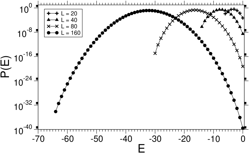
Figure 2: Normalized DOS of different randomly generated RNA sequences. Lines are guides to the eyes only.

The dynamic programming algorithm for the partition function can be easily generalized to exact DOS calculations in $\mathcal{O}(L^{5})$ time complexity. This is possible because the energy occurs in multiples of an energy “quantum” (the energy of a pair). Then the canonical partition function at inverse temperature $\beta=\ln z$ of the subproblems $r_{i}\cdots r_{j}$ can be written as a polynomial in $z$: $\tilde{Z}_{i,j}(z)=\sum_{n=0}^{n_{\max}}g_{i,j}(E_{n})\cdot z^{n}$. In this notation the index $n$ is the number of pairs and hence, using our simple energy model, $E_{n}=-e_{p}n=-n$. The coefficients $g_{i,j}(E_{n})$ of this polynomials yield the DOS of the subproblems and the full DOS is given by $g(E_{n})=g_{1,L}(E_{n})$.

The generalization of Eq. (3) is given by

$$\tilde{Z}_{i,j+1}(z) =\tilde{Z}_{i,j}(z)+\sum_{k=i}^{j-h_{\textrm{min}}}\,\tilde{Z}_{i,k-1}(z)\,c_{r_{k},r_{j+1}}(z)\,\tilde{Z}_{k+1,j}(z)$$

where $$c_{r_{k},r_{j+1}}(z) =\cases{z&if $r_{k}$ and $r_{j+1}$ are complementary\\ 0&otherwise}$$

with similar boundary conditions $\tilde{Z}_{i,i}(z)=1$ and $\tilde{Z}_{i,i-1}(z)=1$. Since the numbers $Z_{i,j}$ are replaced by polynomials and multiplications between these objects are involved, the time complexity increases to $\mathcal{O}(L^{5})$. In Fig. 2 the normalized DOS $P(E)=\frac{1}{\sum_{E^{\prime}}g(E^{\prime})}\cdot g(E)$ for four different randomly generated RNA sequences of lengths between $20$ and $160$ are illustrated. Note that the DOS depends on the disorder realization, i.e. on the sequence and that the DOS can be obtained exactly over the full range of energy values, easily resulting in normalized densities of $10^{-40}$. Hence, RNA secondary structure is a complex-behaving model with quenched disorder that can be treated exactly for each realization. This makes it very valuable for the study of the dynamics of algorithms, like MC approaches, as considered in the next section.

3 Monte Carlo methods to obtain the DOS

In this section we review the MC algorithms used in this study. All algorithms are based on a Markov chain in the space of structures with a fixed sequence ${\mathcal{R}}$, starting with an empty structure. For simplicity, the dependence of all quantities on ${\mathcal{R}}$ is not stated explicitly below. Before explaining the algorithms in details, a few general statements are made, which apply to all algorithms studied here.

3.1 Three classes of proposals

Given a structure $\mathcal{S}$, a single MC proposal consists of selecting a candidate structure $\mathcal{T}$ from its local neighborhood. The neighborhood of $\mathcal{S}$ is defined here by a removal or insertion of a bond, i.e. two kind of MC moves are imposed. The proposal is accepted according to the Metropolis acceptance rule

$$r=\min\left\{1,w(E(\mathcal{T}))/w(E(\mathcal{S}))\right\},$$ (4)

where $w(\cdot)$ is a weight function which depends on the energy $E(\cdot)$ of a structure given by Eq. (2). This ratio of weights between the new and the old structure is implementation dependent. For example it depends on the temperature in the canonical ensemble or on the weights of a generalized ensemble.

At the beginning of the simulation a list of all $N_{\text{possible}}$ possible pairs $\{(i,j)\}$ is created. These pairs are compatible to the energy model ($e(r_{i},r_{j})<\infty$) and have sufficient distance $h_{\textrm{min}}$ along the sequence. Note that there are $\mathcal{O}(L^{2})$ of possible pairs.

This class of pairs can be divided into three classes at each stage of the simulation in terms of the n-fold way [31]. The first class are the active pairs, i.e. that pairs that are currently bonded. The class of inactive pairs can be divided into two subclasses, namely allowed pairs, which can be inserted to the current structure according to the energy model, and currently forbidden pairs, which would lead to pseudo knots for example. Structures which include forbidden pairs (which will never occur in our simulations), we call forbidden as well. Formally, structures, which have forbidden pairs, have zero weight in Eq. (4).

Active pairs are associated with an energy change of $\Delta E=1$, allowed pairs with $\Delta E=-1$ and forbidden pairs with $\Delta E=\infty$. The number of members in the classes given structure $\mathcal{A}$ are denoted by $N(\mathcal{A},+1)$, $N(\mathcal{A},-1)$ and $N(\mathcal{A},0)$ for active, possible and forbidden pairs respectively.

A secondary structure is represented as list of links to the static array of possible pairs. Then the simulation requires some bookkeeping of the lists for all three classes. For this purpose it makes sense to setup a list of cross-links between all pairs indicating incompatibility, i.e. a list of pairs of pairs that lead to pseudo knots, when they both are inserted at the same time.

The most simple approach, ensuring detailed balance, would work in the following way. For each MC step, select one pair among all possible pairs. Then

• If the pair is allowed or active, insert or remove (i.e. “flip”) it from the structure with probability given by (4). Hence, for standard MC, an allowed pair would be inserted always, and an active pair removed with some probability smaller than one.

• If the pair is forbidden, do nothing.

However in “dense” systems this algorithm gets stuck very quickly because in many cases a forbidden pair would be selected in almost all cases, because in this case the number of active and allowed pairs is $\mathcal{O}(L)$ only. In order to speed up this algorithm, we use a dynamics, that avoids attempts leading to forbidden pairs and selects pairs from the list of active or possible pairs only. Each of the $N(\mathcal{A},+1)+N(\mathcal{A},-1)$ pairs have the same probability to be selected. The forbidden attempts are taken into account, by advancing the simulation-time clock sufficiently. This kind of dynamics combines a “rejection-free dynamics”, as implemented in the n-fold way [31], with standard acceptance probabilities. Details are presented now.

The dynamics of an algorithm can be seen as a random walk in structure (configuration/state) space. When performing the simulation, one has to account for the waiting times $m$, that the random walker would have stayed in the structure $\mathcal{S}$ due to forbidden transitions in the local environment. It can be computed by following considerations: Let $p$ be the probability that a forbidden pair is selected, given that the random walker sits in state $\mathcal{A}$, i.e.  $p=N(\mathcal{A},0)/N_{\text{possible}}.$ Then probability that the random walk selects a non-forbidden pair in the the current state after $m$ trials is given by

$$p(m)=p^{m}(1-p).$$ (5)

The probability of staying at most $\tau$ time steps can be evaluated via geometric progression:

$$P(\tau)=\mathbb{P}\left[m\leq\tau\right]=\sum_{m=0}^{\tau}p^{m}\cdot(1-p)=1-p^{\tau+1}$$ (6)

In order to assign a waiting time to the current structure one has to draw a random number according to the discrete distribution Eq. (6), i.e.

$$\tau=\lfloor\ln(\zeta)/\ln(p)\rfloor,$$

where $\zeta$ is an uniformly distributed random number and $\lfloor x\rfloor$ denotes rounding down to the next integer.

After the simulation-time clock has advanced by the waiting time, a pair is selected from the set of active and allowed pairs with uniform probability, and the pair is flipped with a probability given by (4). Hence, if the flip is rejected, then the current structure persists. This completes one MC step.

There are two timescales involved. The computer time measures the number of MC steps and the MC time is associated with a physical time scale of the random walker. The first plays the major role in the performance analysis of the algorithms and the latter one gives the correct weight to the visited states.

Next we want to sample three quantities of interest, the energy, a random energy change $\Delta E$ associated with each attempt (regardless if the step is accepted or not) and a random waiting time. To sum it up, we want to sample the sequence

$$(\hat{E}_{1},\Delta\hat{E}_{1},\hat{\tau}_{1}),\ldots,(\hat{E}_{m},\Delta\hat{E}_{m},\hat{\tau}_{m}).$$

In the following we will outline the two MC schemes, that were used to collect data for our estimate. In both cases, we study the evolution on the scale of macrostates, which contain all structures of the same energy. The first approach is based one generating flat histograms for the macrostates, while the second approach estimates the DOS from transition matrices.

3.2 Flat-histogram ensemble

Instead of sampling configurations according to the Boltzmann weight $w(E)\propto\exp(-\beta E)$, flat histogram methods use a different weight function, such that all macrostates are visited with equal probability. A perfect flat histogram ensemble, where $w(E)\propto 1/g(E)$, requires the knowledge of the DOS $g(E)$. As already outlined, many advances had been made to estimate the DOS iteratively, for example Wang-Landau sampling [20, 21]. In a final stage of this algorithm one usually fixes a good approximation of the DOS and performs a production run in an almost flat histogram ensemble. Here we take advantage of the fact that we can obtain the exact DOS for each realization of the disorder. This allows us to measure the performance of the perfectly flat histogram ensemble, which results in an upper bound for other approaches, where an exact DOS calculation is not possible.

3.3 Optimized flat-histogram ensemble

Perfectly flat histogram methods are only optimal in the sense, that all macrostates are visited with equal probability. There might remain large correlations due to the fact that the random walker stays in local minima for a long time. Especially near phase transitions, where the specific heat diverges, a huge amount of computation time is spent. This effect is known as critical slowing down.

This is also related to regeneration of Markov chains in the following sense: An Markov chain is regenerative if there are times $T_{i}$, such that the process after $T_{i}$ becomes independent from times before $T_{i}$. Obviously our model has a regeneration point, whenever the random walk hits the null structure. The path between regeneration points are called tours. Usually the distribution of tour lengths exhibits a heavy tail and only a very small fraction of tours hit one of the ground states. The first-passage time (also called tunneling time) is the time the random walker needs to hit the ground state starting at its last regeneration point. This is an extremal event and, hence the distribution of first-passage times might be, at least approximately, a generalized extreme-value distribution exhibiting a heavy tail.

Small first-passage times increase mixing and performance of the sampler. We will also use round-trip time, which is the tunneling time plus the time needed to go back to regeneration. Since the turn from regeneration to the ground state is much longer than the turn back, first-passage time and round trip equal approximately.

Trebst et al. [22] developed an iterative algorithm to optimize round-trip times in a generalized ensemble. Instead of giving all macrostates the weight $w(E)\propto 1/g(E)$ a different weight function $w^{\text{opt}}(E)$ is chosen, such that the number of round trips between an energy interval $E_{+}$ and $E_{-}$ is maximized.

The equilibrium distribution of the optimized ensemble is proportional to $w^{\text{opt}}(E)\cdot g(E)$, which is not a flat histogram in general. The methods works for both, for Metropolis and n-fold dynamics. Consider the steady state current from $E_{+}$ to $E_{-}$, which is to first order

$$j\propto D(E)\cdot w^{\text{opt}}(E)\cdot g(E)\frac{df}{dE}$$

for a continuous energy. $D(E)$ denotes the local diffusivity at energy level $E$ and $f(E)$ is the fraction of visits at energy $E$, where the last visits to $E_{+}$ has occurred more recently than to $E_{-}$. A sample estimate for $f$ can be made by labeling the random walker with two different labels “$+$” or “$-$”, depending on whether it has visited the state $E_{+}$ or $E_{-}$ most recently. During the simulation a separate energy histogram $H_{\pm}(E)$ for each label is updated and an approximation of $f$ for the given weights is given by

$$\hat{f}(E)=\frac{H_{+}(E)}{H_{+}(E)+H_{-}(E)}.$$

The feedback iteration that converges to the optimized ensemble for Metropolis updates is given by [22]

$$w^{k+1}(E)=w^{k}(E)\cdot\sqrt{\frac{1}{H_{+}(E)+H_{-}(E)}\cdot\frac{df}{dE}}.$$ (7)

For the n-fold way, or as in our case the semi rejection-free dynamics, the iteration has to account for the two intrinsic time scales. Since one aims at optimizing the computer time the iteration scheme Eq. (7) is modified by the factor $\tau(E)$, which is the accumulated waiting time at energy level $E$, in other words

$$w^{k+1}(E)=w^{k}(E)\cdot\sqrt{\frac{1}{H_{+}(E)+H_{-}(E)}\cdot\frac{df}{dE}\cdot\frac{1}{\tau(E)}}.$$ (8)

After each iteration the number of MC steps, which is used to accumulate the histograms, is doubled. The derivative $df/dE$ can be approximated by a polynomial interpolation of $f(E)$ and numerical derivation.

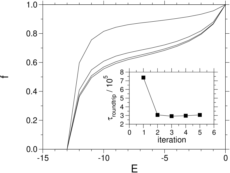
Figure 3: Convergence of $f(E)$ using iteration scheme Eq. (8), shown by lines connecting the data points, for better visibility. The energy weights were optimized between $E_{-}=E_{1}$ (first excitations) and the null structure $E_{+}=0$. Between iteration 4th and 5th no significant difference of $f(E)$ is visible. Inset: Convergence of round-trip times. Lines in the inset are guides to the eyes only.

Since the events for going from a first excited state $E_{1}$ to the ground state $E_{0}$ occur very rarely, the statistics for $f$ might be bad and the iteration scheme Eq. (8) converges slowly, if the complete energy spectrum is considered for the optimized ensemble. However, an optimization over the complete range is not essential and it is sufficient to optimize the ensemble from first excitations $E_{-}=E_{1}$ to the null structure $E_{+}=0$. The link to the remaining weight $w^{i+1}(E_{0})$ can be made by requiring the next iteration to visit either the ground state or the first excitations with equal probability (any other finite fraction will work as well), i.e.

$$w^{i+1}(E_{0}) = w^{i+1}(E_{1})\cdot\frac{g(E_{1})}{g(E_{0})}$$

$$\approx w^{i+1}(E_{1})\cdot\frac{H_{+}(E_{1})+H_{-}(E_{1})}{H_{+}(E_{0})+H_{-}(E_{0})}\cdot\frac{w(E_{1})}{w(E_{0})}.$$

Note that the random walker itself is not restricted to $\left[E_{-},E_{+}\right]$. During each iteration one can measure the round-trip time of the random walker over the full spectrum from $E_{0}$ to the null structure as a quantity which describes the performance. For a small system $L=40$ we compared the performance of the optimization over the full spectrum and the restricted spectrum and found no significant difference in round-trip times. In both cases the round-trip time decreases by a factor of about $2$ already in the second iteration of updating the weights. The effect of decreasing round-trip times becomes more pronounced for larger systems (see Sec. 4).

3.4 DOS through transition matrix estimates

The method, we will examine next, is based on evaluating data from infinite temperature transition matrices. Hence, it has similarities to transition matrix MC (TMMC), which was introduced by Lee and Wang in several publications [32, 33, 34]. In TMMC, one uses an acceptance rate which is more general than Eq. (4). Here we keep the original weights for generalized (flat histogram or optimized) ensemble or simulated annealing (ParQ) dynamics with Metropolis update rules.

The connection between the transition matrix and DOS can be made as follows:

Consider an infinitely long simulation in the canonical distribution at infinite temperature, where all attempts are allowed apart from those that yield forbidden structures. The discrete time and state master equation for the so constructed chain on the level of the macrostates is given by

$$p(E_{j},t+1)=\sum_{E_{i}}Q(j|i)\cdot p(E_{i},t),$$ (9)

where $p(E_{i},t)$ denotes the probability of finding macrostate state $E_{i}$ at time $t$ and $Q(j|i)$ is the macrostate transition matrix, i.e. the probability of jumping to a state with energy $E_{j}$, given that the random walker sits in state with energy $E_{i}$. Since $Q(j|i)$ is stochastic we require that the columns sum to one, i.e. $\sum_{j}Q(j|i)=1$ for all $i$. The stationary distribution of Eq. (9) is the wanted DOS $g(E)$. For a known $Q(j|i)$ this can either be computed via solving the eigenvalue problem Eq. (9), or iterating the equation

$$p^{(k+1)}(E_{j})=\sum_{i}Q(j|i)\cdot p^{(k)}(E_{i})$$ (10)

starting with arbitrary initial values $p^{(0)}$ [35].

Next we discuss how $Q$ can be estimated from MC data on attempted moves. $Q(j|i)$ is related to the microstate transition matrix $\Gamma(\mathcal{B}|\mathcal{A})$, which is 1 if two non-forbidden structures are connected by a flip of a pair, and to $N(\mathcal{C},\Delta E)$:

$$Q(j|i) = \frac{1}{C_{i}}\sum_{\mathcal{A}}\left(\sum_{\mathcal{B}}\Gamma(\mathcal{B}|\mathcal{A})\cdot\delta_{E(\mathcal{B}),E_{j}}\right)\cdot\delta_{E(\mathcal{A}),E_{i}}$$ (11)

$$= \frac{1}{C_{i}}\sum_{\mathcal{A}}N(\mathcal{A},E_{j}-E(\mathcal{A}))\cdot\delta_{E(\mathcal{A}),E_{i}}$$

where $\delta_{i,j}$ is the Kronecker symbol. The $C_{i}$’s are chosen such that $Q(j|i)$ is stochastic.

An sample estimate of $Q(j|i)$ can be made [36, 26] from MC data on attempted steps and waiting times: In the matrix $\hat{W}(j|i)$ we count the number of attempted moves from $i$ to $j$. Since our approach considers only flips of single pairs, $\hat{W}$ is nonzero only for $j=i-1,i,i+1$. During the simulation $\hat{W}(i\pm 1|i)$ is incremented by one for all proposed transitions (from $i$ to $i\pm 1$), while $\hat{W}(i|i)$ is always incremented by the waiting time.

Even though the configurations have not to be drawn from a microcanonical distribution definitely (one might have a canonical distribution, a mixture of canonical distributions or a generalized ensemble in mind), we require the samples to fulfill the microcanonical property, namely that the probability or weight of a structure $\mathcal{C}$ on energy $E(\mathcal{C})$ only. That means all states with fixed energy are have equal probability. That condition is a crucial point. It was shown that it is automatically fulfilled, when detailed balance is guaranteed [37]. Simulated annealing violates detailed balance explicitly and therefore it is hard to prove, that ParQ yields the correct result. We will examine this issue in Sec. 5.5.

3.5 ParQ: Estimating the transition matrix

Figure 4: Specific heat as a function of the temperature, shown for two realization of length $L=80$ with a typical (solid line) and a large (dashed) ratio $g(E_{1})/g(E_{0})$. Inset: low temperature decay rate of the reduced specific heat is the same for all realizations $c/\beta^{2}\sim\mathrm{e}^{-\beta}$. Dotted lines show some other realizations.

The ParQ [36, 26] algorithm combines ideas from simulated annealing [38, 39] and TMMC. Instead of estimating the transition matrix from an equilibrium simulation the temperature is lowered according to a certain protocol. The acceptance rule is the usual Metropolis one

$$r=\min\left(1,\exp[-\beta\Delta E]\right).$$

The advantages of the method is first that no assumption about the DOS is required at the beginning of the simulation. Secondly, in contrast to the Wang Landau method, ParQ is easy to parallelize because many independent runs can be performed simultaneously.

It is required that all regions of interest are visited by the random walker. Therefore the annealing schedule has to be adjusted. Basically there are two ingredients: the functional form of the (inverse) temperature protocol $\beta(t)$ and the start and end value of the temperature $\beta_{1}$ and $\beta_{2}$. At infinite temperature, the random walker is located at the maximum of the DOS (see Fig. 2), which corresponds to simple sampling, where all allowed steps are accepted. In order to go beyond the maximum towards the unfolded RNA, i.e. for increasing the energy, one has to chose a negative temperature. For the opposite direction, towards the ground state, the temperature has to be positive and finite. The simplest annealing schedule is a linear increase of $\beta$ from $\beta_{1}<0$ to $\beta_{2}>0$. However this kind of cooling schedules might not be optimal. Therefore we also checked two other forms, where the inverse temperature is first increased from $\beta_{1}$ to a certain positive value above the critical temperature, say $\beta=1$ in a linear fashion and then the system is cooled down either linearly or exponentially in $T$. We will denote this three schedules as inverse (INV), linear (LIN) and exponential (EXP) cooling respectively and compare the performance of the three methods later on.

For infinite long simulations, i.e. infinite slow cooling, the sampling approaches the standard Metropolis sampling and the method of estimating the the transition matrix in this way becomes exact, because the microcanonical property is fulfilled. Unfortunately, the convergence for a finite number of cooling steps but infinite number of runs has not been proved so far.

The temperature range $[\beta_{1},\beta_{2}]$ should be chosen, such that the energy fluctuations vanish sufficiently. This can be assessed by considering the specific heat capacity $c=\beta^{2}(\left<e^{2}\right>-\left<e\right>^{2})$ [39] obtained from exact calculations, where $e$ is the energy per pair of bases, i.e. $e=E/L^{2}$. For the usual case, where the DOS is not a priori $c(\beta)$ known, has to be estimated from a few primary simulations or the temperature range has be estimated in other heuristic ways.

The specific heat capacity for two different realizations of length $L=80$ is shown in Fig. 4. For these two examples we used temperature ranges $[-10,10]$ and $[-10,15]$, respectively. Note that the decay of $c$ in the low temperature limit $\beta\rightarrow\infty$ (see inset of Fig. 4) can be understood very well [40]: At low temperatures the partition function is dominated by the ground state and first excitations only and hence

$$\frac{c}{\beta^{2}}=\left<e^{2}\right>-\left<e\right>^{2}\sim(E_{0}-E_{1})^{2}\cdot\frac{g(E_{1})}{g(E_{0})}\cdot\mathrm{e}^{-\beta(E_{1}-E_{0})}$$

Since $E_{1}-E_{0}=1$ for all realization in our simple model the specific heat capacity decays as $C/\beta^{2}\sim\exp(-\beta)$ and only the prefactor is dominated by large sample to sample fluctuations of $g(E_{1})/g(E_{0})$ (see Sec. 5.1). A large value of this ratio implies a narrowed peak of the specific heat capacity and hence increasingly slow relaxation times. In more complex systems, such as RNA secondary structure with hybrid energy models [11], even the exponent may vary because of variable energy difference between ground states and first excitations.

4 Analysis of convergence

In order to assess the performance of different MC algorithms, we conducted simulations using the different approaches described above. We compared the performance using a fixed realization of length $L=80$ and small ground-state degeneracy, i.e. a large ratio $g(E_{1})/g(E_{0})$. This ratio is somehow a measure for the amount of meta-stable states. It is a purely local property and does not depend on large structures of the energy landscape. Those instances with a large value of this ratio are the expected to be “hardest” instances by comparison with spin glasses [41, 42], and indeed confirmed by our results, see Sec. 5. For all simulations techniques, $5\times 10^{9}$ MC steps were used totally. We performed various independent simulations (25 for ParQ and the optimized ensemble and 16 for the flat histogram random walker) with different seed values but fixed realization.

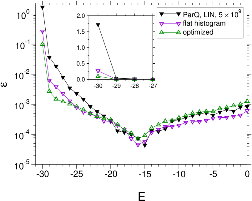
Figure 5: Relative error of the DOS of a low degeneracy of ground states using flat histogram ensemble, optimized ensemble and ParQ with fixed cooling rate ($5\times 10^{10}$ steps per run). The inset shows the same data with a linear ordinate. The ratio $g(E_{1})/g(E_{0})$ for the realization was $3120649/16$, which is larger than typical values. Lines are guides to the eyes only.

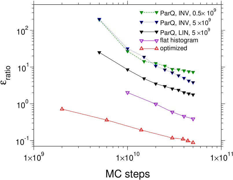
Figure 6: Rate of convergence of the relative error of the ratio $g(E_{1})/g(E_{0})$ for different simulation methods: ParQ for inverse and linear cooling schedule using $500\times 10^{6}$ and $5000\times 10^{6}$ steps per run. For $5000\times 10^{6}$ steps no significant difference between inverse and linear cooling is visible. Flat histogram and the optimized ensemble sampling perform much better than ParQ. The ratio $g(E_{1})/g(E_{0})$ for the realization was $3120649/16$, which is larger than for typical instances.

The ParQ result was obtained by a linear and inverse temperature schedule with a temperature range from $\beta_{1}=-10$ to $\beta_{2}=15$ (data for the inverse schedule is not shown in Fig. 5) and the overall $5\times 10^{10}$ MC steps were separated in 10 independent runs of length $5\times 10^{9}$.

The so approximated DOS obtained from ParQ was used as an input for the flat-histogram method, as well as for the first iteration of the optimized flat-histogram method. This might be a realistic procedure, because the DOS is not known in general. We used $E_{-}=E_{1}$ and $E_{+}=0$. For the standard flat-histogram approach, no further adjustment had to be made, hence the histograms could be sampled using this input using all available MC steps. For the optimized ensemble, to optimize the function $f(E)$, describing the history of the walker with respect to $E_{+}$, we applied $10^{9}$ MC steps for the first iteration and then doubled this number always for each following iteration. Similar to the $L=40$ system (Fig. 3), the estimate of $f(E)$ converged after only 5 iterations. Hence the optimal weights where found quickly. Via this optimization, the round-trip time decreased by a factor of about $4$. The remaining $1.9\times 10^{10}$ steps, where the weights were kept fixed, could be used to gather the final histogram.

To compare the power of the different algorithms, we considered the relative error of the MC approximation with respect to the exact solution $\epsilon(E)=\left|\hat{g}(E)-g(E)\right|/g(E)$, where $\hat{g}$ is the sample estimate obtained either by iteration of Eq. (10) or via the energy histogram, depending on the algorithm. The averaged $\epsilon(E)$ is shown in Fig. 5.

A second quantity, which gives a relevant measure of performance is the sample error of ratio between first excitations and ground states

$$\epsilon_{\text{ratio}}=\frac{\left|\hat{g}(E_{1})/\hat{g}(E_{0})-g(E_{1})/g(E_{0})\right|}{g(E_{1})/g(E_{0})}.$$

This quantity as a function of MC steps is shown in Fig. 6.

¿From Fig. 5 and Fig. 6 one can learn that in the high energy region were only a few sites are connected by bonds the flat histogram method clearly outperforms the other methods, whereas in the relevant low energy region the optimized random walker seems to be best. The most significant difference between the methods is located at the ground state of the system, where the ParQ method is not very accurate. Also the rate and form of the annealing schedule affects the performance: The linear schedule seems to outperform the inverse schedule and, as expected, few long runs beat many short ones.

Note that Fig. 5 and Fig. 6 are worst case scenarios, because we picked out a sample, where the ratio $g(E_{1})/g(E_{0})$ is very large, i.e. there are many meta-stable states that might be separated by large barriers from ground states. We also performed the same kind of simulations for a typical realization of the same length, where $g(E_{1})/g(E_{0})$ is relatively small. The errors of the ratio decrease by a factor of 9.5, 35 and 39 for the ParQ, flat histogram and optimized ensemble method respectively.

In order to check, if the qualitative ranking of the methods, i.e. $\epsilon_{\text{ratio}}^{\text{optimized}}<\epsilon_{\text{ratio}}^{\text{flat}}<\epsilon_{\text{ratio}}^{\text{ParQ,LIN}}$, is a general feature of the system we generated an ensemble of 2000 realizations of length $L=40$ and performed the same kind of simulations as before with $5\times 10^{7}$ steps for all simulations. In the majority of the cases (59%) we find the same kind of ranking and second most frequently (33%) a ranking of $\epsilon_{\text{ratio}}^{\text{flat}}<\epsilon_{\text{ratio}}^{\text{optimized}}<\epsilon_{\text{ratio}}^{\text{ParQ,LIN}}$. Only in $2\%$ percent of the cases ParQ outperforms one of the generalized ensemble methods. Sample averages of $\epsilon_{\text{ratio}}^{\text{optimized}}$, $\epsilon_{\text{ratio}}^{\text{flat}}$ and $\epsilon_{\text{ratio}}^{\text{ParQ,LIN}}$ were $0.030$, $0.055$ and $0.551$ respectively. Probably these differences increase for larger systems.

We also checked that linear cooling is better than the other two alternatives in $53\%$ of the cases (exponential and inverse cooling only $15\%$ and $31\%$ respectively).

5 Correlation between algorithmic and structural complexity

As already mentioned the performance strongly depends on the ratio $g(E_{1})/g(E_{0})$, which was also obtained in $\pm J$ spin glasses [41, 42]. In this section we want study the distribution of this ratio and its relationship to the performance of MC algorithms. We also check if there is a correlation between the degree of ultrametricity at finite temperature and performance.

5.1 Ratio between number of first excitations and groundstates

For the usual 2d $L\times L$ Ising ferro magnet without disorder it is obvious, that the ratio $g(E_{1})/g(E_{0})$ scales as $L^{2}$, because there are exactly $L\times L$ possibilities to excite the ground state by one single spin flip. In our model, RNA secondary structure, the scaling behavior can not be obtained with such simple arguments.

Hence, we generated ensembles of up to $40,000$ realizations for sequence lengths between $L=20$ and $L=1021$ sampled the distribution of $g(E_{1})/g(E_{0})$. Even though the transfer matrix algorithm is polynomial, the computations of systems larger than $L=320$ become very time consuming. Therefore we only computed the number of ground states and first excitations instead of the complete energy spectrum. This can be achieved by truncations of the polynomials in the transfer matrix after the term of the second largest power.

Empirically we find a generalized extreme-value distribution (see Fig. 7 ), whose cumulative distribution function is given by

$$\mathbb{P}\left(\frac{g(E_{1})}{g(E_{0})}\geq x\right)=\exp\left[-\left(1+\xi\,\frac{x-\mu}{\sigma}\right)^{-1/\xi}\right],$$ (12)

similar as in [42].

The parameters of the distribution $\mu$ (location), $\xi$ (shape) and $\sigma$ (scale), were obtained through a maximum likelihood fit using the FORTRAN program by Hosking [43, 44]. The resulting probability density functions (pdf) and the scaling behavior of the fit parameters are shown in Fig. 7.

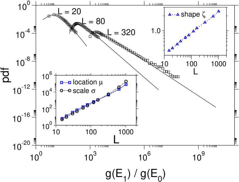
Figure 7: Density distribution of the ratio $g(E_{1})/g(E_{0})$ for different sequence lengths. Squares indicate binned data. The largest errorbar is as large as the symbols.
Insets: scaling of the location, scale and shape parameter on a double logarithmic scale.

The qualities of the maximum likelihood fits were not good enough to be convinced that the data indeed follows Eq. (12), especially for large sequences. This is also supported by small p-values of Kolmogorov-Smirnov tests. But the data at least allows to distinguish between an exponential and algebraic growth of the location and scale parameter: Similar as for the $\pm J$ model [14] we find an algebraic behavior of location and shape parameter $\mu(L)=A\cdot L^{z_{\mu}}$ and $\xi(L)=B\cdot L^{z_{\xi}}$ with an exponents of $z_{\mu}=2.1(1)$ and $z_{\xi}=2.4(9)$. Although the quality of the fit is not very high (as can be seen already in the lower left inset of Fig. 7 where the empirical data do not follow a straight line in the log-log plot), an exponential scaling can be safely excluded by our data.

5.2 Ultrametricity of the phase space

The study of ultrametric spaces dates back many decades and has entered the physical literature in the context of spin glass theory (see [45] and references therein).

Higgs found evidence that RNA secondary structures exhibit an ultrametric structure [5] at low temperatures. The existence of a phase transition was then confirmed numerically by Pagnani et al. [7] by considering the width of the overlap distribution and then examined by other authors using droplet theory [9], the $\epsilon$-coupling method [10] and renormalized field theory [12].

Ultrametricity can be detected by considering the “distance” between two structures drawn from a canonical ensemble at a given temperature. Using the transfer matrix $Z_{i,j}$ it is possible to draw states directly without performing Markov chain MC [5]. It is also possible to enumerate ground states or, if the degeneracy is too large to enumerate, one may sample them equally likely [8].

Given two structures $\mathcal{A}$ and $\mathcal{B}$, their overlap is defined by $q_{\mathcal{A}\mathcal{B}}=\frac{1}{L}\sum_{n=1}^{L}\delta_{{b^{\mathcal{A}}_{n}},b_{n}^{\mathcal{B}}}$, where

$$b^{\mathcal{S}}_{i}=\cases{j&{ if } $(i,j)\in\mathcal{S}$\\ 0&{ otherwise}}$$

The normalized distance between $\mathcal{A}$ and $\mathcal{B}$ is given by $d(\mathcal{A},\mathcal{B})=1-q_{\mathcal{A}\mathcal{B}}$.

An ultrametric space $M$ is defined by following axioms:

1. $0\leq d(\mathcal{A},\mathcal{B})$ and $d(\mathcal{A},\mathcal{B})=0\iff\mathcal{A}=\mathcal{B}$

2. $d(\mathcal{A},\mathcal{B})=d(\mathcal{B},\mathcal{A})$

3. $d(\mathcal{A},\mathcal{C})\leq\max\left\{d(\mathcal{A},\mathcal{B}),d(\mathcal{B},\mathcal{C})\right\}$ ,

for all $\mathcal{A}$, $\mathcal{B}$, $\mathcal{C}\in M$. Note that every ultrametric space is a metric space.

A direct consequence is that each triangle is isosceles, i.e. the two largest sides of a triangle are of equal length. This property provides a numerical criterion for the detection of ultrametricity [5]: The degree of ultrametricity can be estimated by the difference of the two largest distances of a set of candidate triangles. This quantity, which is denoted as $s$, vanishes in perfectly ultrametric spaces and become small in approximately ultrametric spaces.

There might be different reasons, why $s$ may vanish in the thermodynamic limit and therefore one has to filter real ultrametricity against trivial one. E.g. in the high temperature phase, $s$ also scales as $N^{-1/2}$ and the maximum size of $s$ is limited by the triangle equation. To distinguish from this trivial ultrametricity, Higgs samples [5] sets of “uncorrelated” triangles by computation of three independent distances $d(\mathcal{A},\mathcal{B}),d(\mathcal{C},\mathcal{D}),d(\mathcal{E},\mathcal{F})$. If these distances fulfill the triangle inequalities, i.e. $d(\mathcal{A},\mathcal{B})\leq d(\mathcal{C},\mathcal{D})+d(\mathcal{E},\mathcal{F})$ and for all other combinations of the distances, the difference between the two largest distances is computed. Finally the average of the differences taken over all valid uncorrelated triangles $s_{\text{uncor}}$ is computed. Non-trivial ultrametricity should emerge faster than the trivial ultrametricity obtained from uncorrelated distances. Hence $s^{\ast}=s/s_{\text{uncor}}$ should vanish in the presence of an ultrametric structure in the thermodynamic limit.

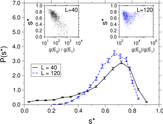
Figure 8: Distribution of deviations from ultrametricity at $T=0.125$. Inset: scatter plot between $g(E_{1})/g(E_{0})$ and $s^{\ast}$.

In principle one should distinguish the finite temperature and zero temperature behavior in complex phase, as already pointed out in [8]. Using direct sampling of ground states a “non-trivial” overlap distribution at zero temperature could be ruled out by numerical extrapolation. This implies that grounds states alone are not ultrametric. For this reason we considered only finite temperature states, where the overlap distribution is non-trivial [7] and evidence for an ultrametric phase space still remains. This arguments are also supported by the observation, that the temperature dependent values of $s^{\ast}$ have a minimum below the critical and above zero temperature. However $s^{\ast}$ decreases only slowly with system size [5] and therefore the quality of the data have to be used with care (see for example [46] an the related comment [47]). Hence, much larger systems sizes, which are unfortunately out of reach, would be necessary to decide this question finally. However, since our model has properties of a mean field model, an ultrametric space would be not surprising (in contrast to the finite dimensional model considered in [46, 47]).

In Fig. 8 we illustrate the distribution of $s^{\ast}$ over many realizations for $L=40$ and $L=120$ at a temperature $T=0.125$ slightly below the transition. As expected, the transition moves a bit to towards small values of $s^{\ast}$ for increasing system size. In the small system the correlations between the ratio $g(E_{1})/g(E_{0})$ and $s^{\ast}$ (see insets) are stronger. We assume that this is an finite-size effect, because this effect is weaker for larger systems.

We will quantify these correlations in the following section.

But first we explain an alternative approach, where ultrametric spaces can also be detected and analyzed by clustering low distance configurations in hierarchical groups. The clustering algorithm used in this paper is Ward’s algorithm [48], an agglomerative hierarchical matrix updating algorithm, also called minimum variance method as it is designed to minimize the variance of the constructed clusters. The algorithm works as follows. Initially each configuration forms a cluster of its own, and the distance matrix $d_{ab}$ with the distances of all pairs of clusters(each containing one configuration) is calculated using e. g. the above defined distance. Then in each step the two clusters $p$ and $q$ with the smallest distance are fused to form a new cluster $t$. The distance matrix is updated using

$$d_{rt}=\frac{(n_{r}+n_{p})d_{rp}+(n_{r}+n_{q})d_{rq}-n_{r}d_{pq}}{n_{r}+n_{t}}$$ (13)

where $r$ refers to any of the other clusters left unchanged in the current step and $n_{x}$ is the number of configurations in cluster $x$. This is repeated until only one cluster remains which now contains all configurations. Afterward, one can re-order the configurations according to the cluster hierarchy obtained in the fusing process, and draw a color-coded visualization of the distance matrix. In Fig. 9 four different distance matrices for different realizations and temperatures are illustrated. As one can see, a clear cluster structure emerges only at low temperatures, but a clear correspondence between the ultrametricity $s^{\ast}$ and the visual impression cannot be made. Note that one can apply a clustering algorithm to any set of data, hence also to non-ultrametric ones. There are quantitative methods, which test how much the tree imposed by the clustering algorithm correlates with the distances in the data. Here, we have just used the visual impressions obtained by looking at the matrices. Furthermore, in the last section we will use the so detected clusters to check whether all ground states are visited with equal probability.

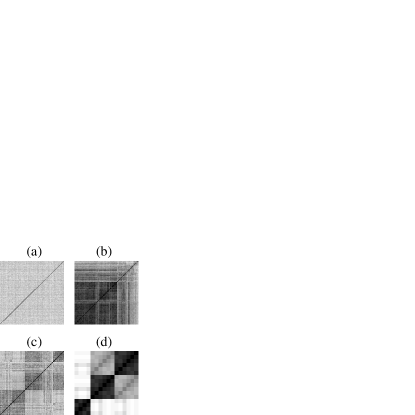
Figure 9: Hierarchical structure of the states illustrated by distance matrices. Darker grey scales correspond to large overlaps. (a) $L=120$ at $T=2$. No hierarchical structure could be detected ($s^{\ast}\approx 1$)
(b) $L=120$ at $T=0.125$ for a realization exhibiting a weak ultrametricity ($s^{\ast}\approx 0.74$)
(c) $L=120$ at $T=0.125$ for a realization exhibiting stronger ultrametricity ($s^{\ast}\approx 0.45$)
(d) $L=40$ at $T=0.0$ for a realization having low ground-state degeneracy ($g(E_{1})/g(E_{0})=14638/16$) Deviation from ultrametricity was $s^{\ast}\approx 0.5$. Realization (d) was also used in section 5.5. The corresponding dendrogramm is illustrated in Fig. 13.

5.3 Distribution of tunneling times of the flat histogram random walker

We measured the tunneling time for the flat histogram random walker for sequence lengths up to $120$. Note that larger systems become infeasible if one wants to span a large energy interval, which we need to when studying tunneling time distributions. Already for $L=120$ we found tunneling times fluctuating ranging in real time between seconds and days on a modern CPU.

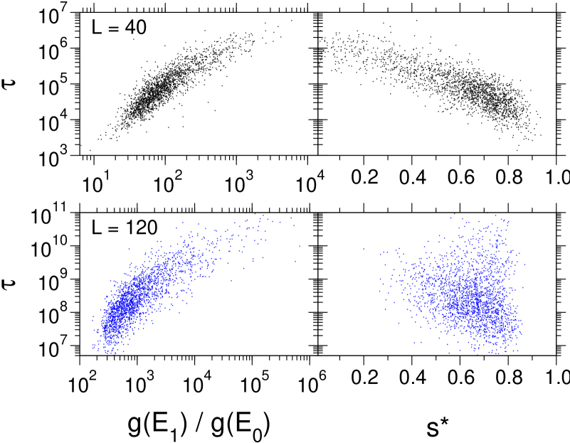
Figure 10: Left column: Scatter plot between the ratio $g(E_{1})/g(E_{0})$ and tunneling time of the flat histogram sampler for $L=40$ (upper) and $L=120$ (lower).
Right column: Scatter plot between deviation from ultrametricity and tunneling time of the flat histogram sampler for $L=40$ (upper) and $L=120$ (lower).

There is a strong correlation between $g(E_{1})/g(E_{0})$ and the tunneling time, see Fig. 10. We found that this is in particular true when this ratio is much larger than all other ratios between neighboring energy densities. The performance of the algorithm is then dominated by the rare event of finding a ground state when starting from a first excitation. Two scatter plots of the ultrametricity index $s^{\ast}$ versus tunneling time are shown in Fig. 10. Hence, whether there is a true correlation between tunneling time $\tau$ and degree of ultrametricity $s^{\ast}$ is not clear, because for larger system the correlation appears to be rather weak.

To investigate the issue of correlations between static measures and computational hardness more quantitatively we calculated the empirical Pearson correlation coefficients for all pairs of quantities $\log\tau$, $\Delta S=\log\left(g(E_{1})/g(E_{0})\right)$ and $s^{\ast}$, which results in

$$\hat{\rho}=\left(\begin{array}[]{ccccccc}&\vline&\log\tau&\Delta S&s^{\ast}_{(T=0.125)}&s^{\ast}_{(T=0.033)}\\ \hline\cr\log\tau&\vline&1&0.89&-0.40&-0.33\\ \Delta S&\vline&&1&-0.37&-0.30\\ s^{\ast}_{(T=0.125)}&\vline&&&1&0.87\\ s^{\ast}_{(T=0.033)}&\vline&&&&1\end{array}\right)$$

for $L=40$ and

$$\hat{\rho}=\left(\begin{array}[]{ccccccc}&\vline&\log\tau&\Delta S&s^{\ast}_{(T=0.125)}&s^{\ast}_{(T=0.033)}\\ \hline\cr\log\tau&\vline&1&0.82&-0.18&-0.16\\ \Delta S&\vline&&1&0.02&-0.13\\ s^{\ast}_{(T=0.125)}&\vline&&&1&0.28\\ s^{\ast}_{(T=0.033)}&\vline&&&&1\end{array}\right)$$

for $L=120$. As pointed out in Sec. 5.2 there is a correlation between $s^{\ast}$ and $\Delta S$, at least for smaller systems. In order to check if there is a direct correlation between ultrametricity and tunneling time we computed the partial correlation $\hat{\rho}_{\log\tau,s^{\ast}\cdot\Delta S}$ [49], which leads to no significant values for all sequence lengths we considered here. Hence this correlation might be trivial, because it is induced by correlation of the ratio $g(E_{1})/g(E_{0})$ and tunneling time.

This means, although ultrametricity is usually considered as a landmark of complex and glassy systems, at least for the behavior of RNA secondary structures it is not related to the dynamic glassy behavior seen in MC simulations. We believe that the effect of ultrametricity is superimposed by the large number of metastable states.

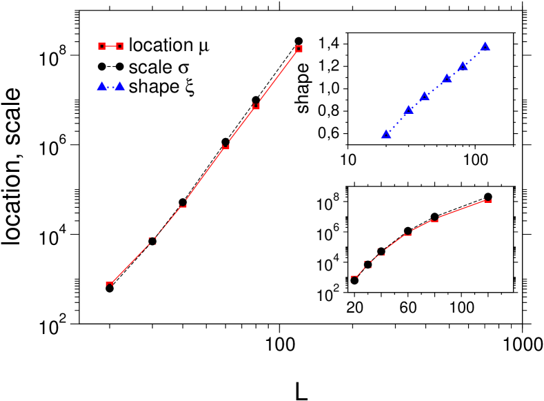
Figure 11: Scaling of the location (square symbols) and scale parameters (circles) on the tunneling time. Insets: scaling of the shape parameter using a logarithmic abscissa (top) and scaling of the location and scale parameters using a logarithmic ordinate (bottom).

We fitted also the distributions of the tunneling time to a generalized extreme-value distribution Eq. (12) and analyzed the scaling of the parameters. Location and scale parameter have almost the same algebraic dependence on the sequence length, see Fig. 11. As can be seen on the semi-logarithmic plot in the bottom inset in Fig. 11 an exponential scaling can safely be excluded (at least on the length scale up to $120$). The exponent describing the power-law is roughly $z\approx 7$. On the other hand, the shape parameter seems to scale logarithmically in sequence length, see upper inset in Fig. 11. With the same arguments as in Sec. 5.1, we cannot exclude that the distribution deviates from a generalized extreme-value distribution.

These results differ from the $\pm J$ Ising model, where an exponential tunneling time was observed. On the other hand, they are similar to the fully frustrated Ising model, investigated by Dayal et al. [42] They argued, that sub-exponential growth of tunneling times and of the ratio $g(E_{1})/g(E_{0})$ stem from a smaller growth of the number of meta-stable states. These results suggest that the model of RNA is dynamically “simpler” than $\pm J$ spin glasses and has a similar complexity as the fully frustrated model.

On the other hand sample to sample fluctuations are much larger than in the $\pm J$ model, as can be seen by comparing the shape parameter in the range of investigated system sizes. For the largest systems in [42], the scaling parameter was about $0.9$. Hence, although typically RNA instances are not so hard for an MC algorithm, compared to $\pm J$ spin glasses, there is larger fraction of rare hard instances for RNA secondary structures.

5.4 Distribution of MC errors of ParQ and the optimized ensemble random walker

Next the correlation between sampling errors of the ratio $g(E_{1})/g(E_{0})$, the value of the ratio itself, and the degree of ultrametricity was considered (see Fig. 12). We used the ensemble of realizations of length $L=40$, which was already used in Sec. 4.

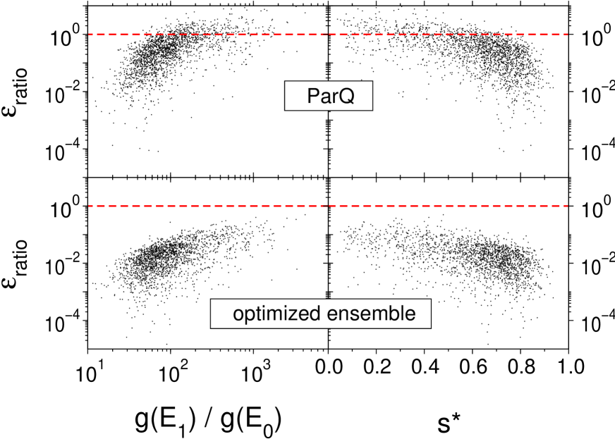
Figure 12: Correlation between the ratio $g(E_{1})/g(E_{0})$ and the error of the ratio for ParQ using linear cooling (upper left) and optimized ensemble simulation (lower left) as well the correlation between deviation from ultrametricity $s/s_{\text{uncor}}$ and the error (upper right for ParQ and lower right for optimized ensemble). The error for optimized ensemble is about one order of magnitude smaller than for the optimized ensemble simulation.

Again we find a correlation between the ratio and performance, which can be quantified via correlation coefficients. The correlation between the error $\epsilon$ and the log-ration $\Delta S$ was larger using the ParQ method ($\hat{\rho}(\epsilon^{\text{ParQ}}_{\text{ratio}},\Delta S)\approx 0.6$) compared to the correlation for the optimized ensemble ($\hat{\rho}(\epsilon^{\text{optimized}}_{\text{ratio}},\Delta S)\approx 0.5)$. Similar to the preceding section, a significant partial correlation between degree of ultrametricity and sampling errors for fixed log ratio $\Delta S$ could not be detected.

5.5 Are all ground states visited with equal probability?

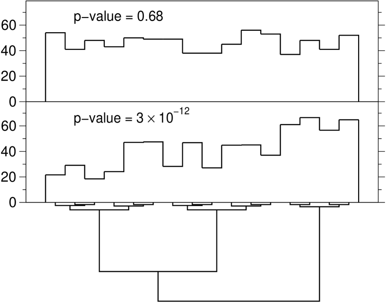
Figure 13: Histograms of visited ground states. upper: optimized ensemble random walker, lower simulated annealing. The Bhattacharyya measures and the corresponding p-values indicate, that simulated annealing does not visit all ground states with equal weight.

¿From Fig. 12 one can also see that the error for the optimized ensemble are one order of magnitude smaller than that of ParQ. Since in both cases the data were obtained from the transition matrix the significant difference must be caused in the underlying MC scheme, probably the non-equilibrium character of ParQ. In order to gain insight to this issue we checked whether the microcanonical property is fulfilled.

In detail we considered histograms of visited ground states for simulated annealing (ParQ) and the optimized ensemble sampler and checked if the histograms were sufficiently flat. A simple and powerful check for the flatness of a histogram is the Bhattacharyya distance measure (BDM) for two given probability mass functions $f(n)$ and $g(n)$ [50], defined as

$$B=\sum_{i}\sqrt{f(i)\cdot g(i)}.$$

This quantity is a measure of the divergence between $f$ and $g$.

The flatness of an empirical histogram of $N$ discrete random variables $X_{1}\cdots X_{N}$ can be measured by replacing $f(n)$ by the sample equivalent $\hat{f}(n)=\sum_{i}\frac{1}{N}h_{n}(X_{i})$, where $h_{n}$ is the indicator function of event $n$, and $g$ is the probability mass function of the null model, i.e. $g(n)=\frac{1}{K}$ with $K$ being the number of categories of the histogram. If $h_{n}$ would be fully flat, one would obtain a BDM of $1$. In empirical data a BDM of $1$ is hardly reached and deviations from $1$ of significant flat distributions depend on $K$ and $N$.

By randomization it is easy to assess p-values, i.e. the probability that a BDM of $B_{0}$ or smaller occurred by pure chance under the assumption that the null model is true [51]: One generates independent histograms with fixed $N$ and $K$ according to the null model and counts the fraction of times, where the BDM is smaller than the observed one. However if the p-values are very small one can implement the method of Wilbur [52] to save some computation time.

Note that the BDM requires the empirical events to be independent. Hence, we generated histograms of independently visited ground states for a small system ($L=40$) and low ground-state degeneracy (we selected a realization exhibiting $K=16$) in the following way: For the optimized ensemble we considered the round-trip time $\tau$ and checked each $\tau$’th if the random walker sits currently at the ground state and, if so, the histogram over all ground states is updated. For simulated annealing, which provides a basis for ParQ, this procedure is not possible in this way, because there is no natural mixing time, which could serve as a thinning interval. Therefore we generated histograms of all visited ground states and renormalized the empirical histograms by considering an effective sample size such that each annealing run has “weight” $1$, i.e. $h_{n}^{\text{eff}}(x)=\frac{N_{\text{annealing}}}{N}h_{n}(x)$, where $N$ is the total number of events.

Note that in the case that the random variable mixes faster than the number of walker’s steps for one annealing run the BDM for the effective histogram might be overestimated (and hence the p-values as well). This would yield false positives. However the opposite case might not occur, because all annealing runs are independent. Therefore the so defined effective histograms can only be used to reject the model, which is exactly what we do here.

The results for both simulation methods are shown in Fig. 13. The upper plot shows one of ten histograms of independent runs for the optimized ensemble random walker, which has a large p-value of $0.68$. The other nine runs yield p-values between $0.007$ and $0.67$ ($0.4(1)$ on average) and hence we can accept the null model. For simulated annealing we find that not all ground states are visited with equal probability (lower plot). The p-values for ten independent runs varied between ($7\times 10^{-13}$ and $5\times 10^{-2}$). Therefore we have to reject the null model, hence these simulated annealing runs visit ground states with a bias. For an even faster cooling schedule we find p-values between $2\times 10^{-24}$ and $2\times 10^{-3}$. The reason for this bias might be that the random walker gets stuck in preferable local minima. The ground-state structure in form of a dendrogram illustrated in Fig. 13 below the histograms supports this argument. The connection between two ground states indicates that these two are merged into one cluster, and the vertical distances are proportional to the Ward-distance, specified in Eq. (13). One can see that within the larges clusters the histogram becomes flatter and that the main source of the non-flatness are differences in sampling between the largest clusters.

6 Conclusion and Outlook

We investigated the relation between static and (MC) dynamic properties of RNA secondary structures and the relation to the performance of different MC algorithms. This model is an ideal test system for this purpose for three reasons: i) The model exhibits quenched disorder and has a complex low-energy landscape, where an interesting dynamical behavior can be expected. ii) It exhibits a static phase transition at finite temperature. iii) The static behavior of the model can be analyzed exactly using polynomial-time partition-function calculations for each single realization of the disorder.

Analyzing the static behavior, we calculated the DOS for ensembles of sequences of different lengths. In particular, we studied the ratio $g(E_{1})/g(E_{0})$, which plays the key role in the complexity of MC methods. The distribution of this ratio could be fitted (but not perfectly) to a generalized extreme-value distribution, similar as previously found for the case of $\pm J$ spin glasses. Location, scale and shape of this distribution scale algebraically with system size, in contrast to $\pm J$ spin glasses. We also computed Higgs’s measure $s^{\ast}$ for the degree of ultrametricity of each realization and used hierarchical clustering approaches to analyze the structure landscape.

For the dynamics, we examined three different MC approaches, which served as basis for evaluating the infinite temperature transition matrix. The nature of the model renders a direct MC implementation very inefficient, hence we also included an $N$-fold way sampling scheme. Flat histogram and optimized ensemble methods provided examples for equilibrium simulations, whereas ParQ is based on simulated annealing, which is an out-of-equilibrium method. In contrast to $\pm J$ model [26] the ParQ method did not yield very accurate results near the ground state and therefore equilibrium methods should be preferred. However, the disadvantage of theses methods is that already suitable initial guesses of the DOS are required. Our simulations show that ParQ can provide such guesses and hence a good strategy might be to combine the ParQ method for a first estimate and use the optimized ensemble method for further refinement.

The tunneling time, as a measure of complexity for the flat histogram random walker, is also distributed according to a generalized extreme-value distribution. The scaling of location and scale parameters seems to be algebraic with an exponent of $z\approx 7$, which differs from the spin-glass model studied in the literature. The scaling of the shape parameter indicate much larger sample to sample than the spin-glass case. Hence, computationally very hard instances occur more often.

Concerning the relation of static properties and dynamical behavior, we found a strong correlation of the MC tunneling times to the value of the ratio $g(E_{1})/g(E_{0})$. A similar correlation was found of the sampling error to $g(E_{1})/g(E_{0})$. On the other hand, we could not find a strong direct correlation between MC tunneling times and degree of ultrametricity of the model. Any numerically observed correlations appear only in a trivial way, i.e. due to a correlation between the degeneracy ratio and $s^{\ast}$. Hence, an ultrametric phase space (a kind of global characterization of the energy landscape), as it seems to be present for RNA secondary structures, does not necessarily lead to a complex dynamics. The presence of meta-stable states, which is only a local property of the energy landscape, appears to be much more important.

Finally we analyzed a possible reason of the failure of the ParQ algorithm: Micro states with equal energy are not visited with equal probability and hence evaluation of the infinite temperature transition matrix does not work correctly. This was not the case for equilibrium methods.

Hence, we have seen that simple models of RNA secondary structures are not only valuable for molecular-biology questions. They are also in particular suitable to study equilibrium and non-equilibrium properties of complex disordered systems and their interdependence. Note that kinetic folding processes are by far more complex than the local update Monte Carlo algorithms used here [27] and a direct biological interpretation of our data is not possible.

Further studies in this field will lead to a better understanding of fundamental equilibrium and non-equilibrium phenomena in disordered systems. Currently, we are also studying aging phenomena for RNA secondary structures and we are hoping to understand them better by comparing with the easily accessible equilibrium.

References

References

- [1] A. P. Young, editor. Spin glasses and random fields. World Scientific, Singapore, 1998.
- [2] K. Binder and W. Kob. Glassy Materials and Disordered Solids: An Introduction to Their Statistical Mechanics. World Scientific, Singapore, 2005.
- [3] A. K. Hartmann and M. Weigt. Phase Transitions in Combinatorial Optimization Problems. Wiley-VCH, Weinheim, 2005.
- [4] M. Henkel, M. Pleimling, and R. Sanctuary. Ageing and the Glass Transition. Springer, Berlin, 2007.
- [5] P.G. Higgs. Overlaps between RNA Secondary Structures. Phys. Rev. Lett., 76:704, 1996.
- [6] I. Tinoco,Jr. and C. Bustamante. How RNA folds. J. Mol. Biol., 293(2):271–281, 1999.
- [7] A. Pagnani, G. Parisi, and F. Ricci-Tersenghi. Glassy Transition in a Disordered Model for the RNA Secondary Structure. Phys. Rev. Lett., 84:2026–2029, 2000.
- [8] A. K. Hartmann. Comment on ”Glassy Transition in a Disordered Model for the RNA Secondary Structure”. Phys. Rev. Lett., 86(7):1382, Feb 2001.
- [9] R. Bundschuh and T. Hwa. Statistical mechanics of secondary structures formed by random rna sequences. Phys. Rev. E, 65(3):031903, Feb 2002.
- [10] M. Mézard F. Krzakala and M. Müller. Nature of the glassy phase of rna secondary structure. EPL (Europhysics Letters), 57(5):752–758, 2002.
- [11] B. Burghardt and A. K. Hartmann. Dependence of RNA secondary structure on the energy model. Phys. Rev. E, 71:021913, 2005.
- [12] Michael Lässig and Kay Jorg Wiese. Freezing of random rna. Physical Review Letters, 96(22):228101, 2006.
- [13] I. Morgenstern and K. Binder. Magnetic correlations in two-dimensional spin-glasses. Phys. Rev. B, 22(1):288–303, Jul 1980.
- [14] L. Saul and M. Kardar. The 2D+/-J Ising spin glass: exact partition functions in polynomial time. Nucl. Phys. B, 432(3):641–667, December 1994.
- [15] J. Villain. Spin glass with non-random interactions. J. Phys. C, 10:1717–1734, 1977.
- [16] M. Mezard. On the glassy nature of random directed polymers in two dimensions. J. Physique France, 51:1831, 1990.
- [17] N. Metropolis, A. Rosenbluth, M. Rosenbluth, A. Teller, and E. Teller. Equation of state calculations by fast computing machines. J.Chem.Phys. 21, 21:1087, 1953.
- [18] J. Lee. New Monte Carlo algorithm: Entropic sampling. Phys. Rev. Lett., 71(2):211–214, Jul 1993.
- [19] B. A. Berg and T. Neuhaus. Multicanonical ensemble: A new approach to simulate first-order phase transitions. Phys.Rev.Lett., 68:9, 1992.
- [20] F. G. Wang and D. P. Landau. Efficient, multiple-range random walk algorithm to calculate the density of states. Phys. Rev. Lett., 86:2050, 2001.
- [21] F. G. Wang and D. P. Landau. Determining the density of states for classical statistical models: A random walk algorithm to produce a flat histogram. Phys. Rev. E, 64:056101, 2001.
- [22] S. Trebst, D. A. Huse, and M. Troyer. Optimizing the ensemble for equilibration in broad-histogram Monte Carlo simulations. Phys. Rev. E, 70(4):046701, 2004.
- [23] C. J. Geyer and E. A. Thompson. Annealing Markov Chain Monte Carlo with Applications to Ancestral Inference. J. Am. Stat. Assoc., 90(431):909–920, sep 1995.
- [24] H. G. Katzgraber, S. Trebst, D. A. Huse, and M. Troyer. Feedback-optimized parallel tempering Monte Carlo. J. Stat. Mech., 2006(03):P03018, 2006.
- [25] N. Rathore, M. Chopra, and J. J. de Pablo. Optimal allocation of replicas in parallel tempering simulations. J. Chem. Phys., 122(2):024111, 2005.
- [26] F. Heilmann and K. H. Hoffmann. ParQ: high-precision calculation of the density of states. Europhys. Lett., 70(2):155, 2005.
- [27] H. Isambert and E.D. Siggia. Modeling RNA folding paths with pseudoknots: Application to hepatitis delta virus ribozyme. Proc Natl Acad Sci U S A, 97(12):6515?6520, 2000.
- [28] R. Nussinov, G. Pieczenik, J. R. Griggs, and D. J. Kleitman. Algorithms for Loop Matchings. J. Appl. Math., 35(1):68–82, 1978.
- [29] M. Zuker. On finding all suboptimal foldings of an RNA molecule. Science, 244:48, 1989.
- [30] P.-G. de Gennes. Statistics of branching and hairpin helices for the dAT copolymer. Biopolymers, 6(5):715–729, 1968.
- [31] A. B. Bortz, M. H. Kalos, and J. L. Lebowitz. A new algorithm for Monte Carlo simulation of Ising spin systems. J. Comp. Phys., 17(1):10–18, January 1975.
- [32] J. S. Wang. Transition matrix Monte Carlo method. Comput. Phys. Commun., 121-122:22–25, 1999.
- [33] J. S. Wang and L. W. Lee. Monte Carlo algorithms based on the number of potential moves. Comput. Phys. Commun., 127(1):131–136, May 2000.
- [34] J. S. Wang, T. K. Tay, and R. H. Swendsen. Transition Matrix Monte Carlo Reweighting and Dynamics. Phys. Rev. Lett., 82(3):476–479, Jan 1999.
- [35] D. W. Stroock. An Introduction to Markov Processes. Springer, Berlin, 2004.
- [36] B. Andresen, K. H. Hoffmann, K. Mosegaard, J. Nulton, J. M. Pedersen, and P. Salamon. On Lumped Models for Thermodynamic Properties of Simulated Annealing Problems. J. Phys. (France), 49:1485, 1988.
- [37] J. S. Wang. Is the broad histogram random walk dynamics correct? Eur. Phys. J. B, 8(2):287–291, March 1999.
- [38] S. Kirkpatrick, C. D. Gelatt Jr., and M. P. Vecchi. Optimization by simulated annealing. Science, 220:671 – 680, 1983.
- [39] S. Kirkpatrick J. J. Schneider. Stochastic Optimization. Springer, Berlin, 2006.
- [40] J. S. Wang and R. H. Swendsen. Low-temperature properties of the Ising spin glass in two dimensions. Phys. Rev. B, 38:4840–4844, 1988.
- [41] S. Adler, S. Trebst, A. K. Hartmann, and M. Troyer. Dynamics of the Wang-Landau algorithm and complexity of rare events for the three-dimensional bimodal Ising spin glass. J. Stat. Mech., 2004(07):P07008, 2004.
- [42] P. Dayal, S. Trebst, S. Wessel, D. Würtz, M. Troyer, S. Sabhapandit, and S. N. Coppersmith. Performance Limitations of Flat-Histogram Methods. Phys. Rev. Lett., 92(9):097201–4, March 2004.
- [43] J. R. M. Hosking. Algorithm AS 215: Maximum-Likelihood Estimation of the Parameters of the Generalized Extreme-Value Distribution. Applied Statistics, 34(3):301–310, 1985.
- [44] A. J. Macleod. Remark AS R76: A Remark on Algorithm AS 215: Maximum-Likelihood Estimation of the Parameters of the Generalized Extreme-Value Distribution. Applied Statistics, 38(1):198–199, 1989.
- [45] R. Rammal, G. Toulouse, and M. A. Virasoro. Ultrametricity for physicists. Rev. Mod. Phys., 58(3):765–, July 1986.
- [46] Pierluigi Contucci, Cristian Giardina, Claudio Giberti, Giorgio Parisi, and Cecilia Vernia. Ultrametricity in the edwards-anderson model. Physical Review Letters, 99(5):057206, 2007.
- [47] Thomas Jorg and Florent Krzakala. Comment on ”ultrametricity in the edwards-anderson model”. arXiv.org, arXiv.org:0709.0894, 2007.
- [48] A. K. Jain and R. C. Dubes. Algorithms for Clustering Data. Prentice Hall, Englewood Cliffs, NJ, 1988.
- [49] A.A. Afifi and S.P. Azen. Statistical Analysis - A Computer Oriented Approach. Academic Press, New York and London, 1972.
- [50] A. Bhattacharyya. On a measure of divergence between two statistical populations defined by their probability distributions. Bull. Cal. Math. Soc., 35:99–110, 1943.
- [51] M.L.J.Scott. Critical Values for the Test of Flatness of a Histogram Using the Bhattacharyya Measure. Technical Report 2004-010, TINA, 2004.
- [52] W.H. Wilbur. Accurate Monte Carlo Estimation of Very Small P-Values In Markov Chains. Comp.Stat., 13:153–168, 1998.