Angular dependence of coercivity in magnetic nanotubes

Abstract

The nucleation field for infinite magnetic nanotubes, in the case of a magnetic field applied parallel to the long axis of the tubes, is calculated as a function of their geometric parameters and compared with those produced inside the pores of anodic alumina membranes by atomic layer deposition. We also extended this result to the case of an angular dependence. We observed a transition from curling-mode rotation to coherent-mode rotation as a function of the angle in which the external magnetic field is applied. Finally, we observed that the internal radii of the tubes favors the magnetization curling reversal.

I Introduction

Since the discovery of carbon nanotubes by Iijima in 1991, Iijima91 intense attention has been paid to hollow tubular nanostructures because of their particular significance for prospective applications. More recently, magnetic nanotubes have been grown SSS+04 ; NCR+05 ; NCM+05 ; Wang05 ; TGJ+06 motivating intense research in the field. Technological applications of such systems require a deep knowledge and characterization of their magnetic behavior. For example, changes in the internal radii are expected to strongly affect the magnetization reversal mechanism LAE+07 and thereby the overall magnetic response. ELA+07 ; SSS+04 The nature of the magnetic tubes may be suitable for applications in biotechnology, where magnetic nanostructures with low density, which can float in solutions, are very desirable. NCR+05

Coercivity is one of the most important properties of magnetic materials for many present and future applications of permanent magnets/magnetic materials, magnetic recording, and spin electronics and, therefore, the understanding of magnetization reversal mechanisms is a permanent challenge for researchers involved in studying the properties of these materials. Recently, Landeros et al. LAE+07 found that, when a magnetic field is applied parallel to the axis of a tube, the curling reversal mode is the dominant magnetization reversal mechanism for tubes with radii greater than $30$ nm. However, the angular dependence of the coercivity in magnetic nanotubes has not been studied yet, in spite of many works on this topic comprising nanowires. WKF+99 ; ZHF+06 In this work we calculate the angular dependence of the coercivity of Ni nanotubes, assuming that the reversal of the magnetization occurs by means of one of two possible modes: magnetization-curling mode ($V$) and coherent-rotation mode ($C$).

Geometrically, tubes are characterized by their external and internal radii, $R$ and $a$, respectively, and length $L$. It is convenient to define the ratio $\beta\equiv a/R$, so that $\beta=0$ represents a solid cylinder and $\beta$ close to $1$ corresponds to a very narrow tube. Besides, we consider an external magnetic field $H_{a}$ applied in a direction defined by $\theta_{0}$, with $\theta_{0}$ the angle of the applied field with the tube axis, as illustrate in Fig. 1.

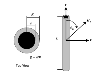
Figure 1: Geometrical parameters of a magnetic nanotube.

In this paper we present an analytical model about the switching modes and fields of infinite extended magnetic nanotubes in dependence of the orientation of the magnetic field versus the nanotube axis. Additionally, experimental data for the switching field of high-aspect ratio Ni nanotubes, when the magnetic field is applied parallel to the tube axis, will be compared with this micromagnetic model.

II Experimental details and results

The high-aspect ratio Ni nanotubes were produced in porous membranes with pore diameters of $180$, $220$ and $260$ nm. The alumina membranes were coated by atomic layer deposition (ALD), that consists of the sequential deposition of thin layers from two different vapor-phase reactants, into a ferromagnetic Ni layer. We used Nickeltocene (NiCp₂) and O₃ as reactants for the deposition of a thin oxide layer, which was reduced after the ALD process into a magnetic layer by annealing at $400$ ⁰C under Ar + 5% H₂ atmosphere. The deposition temperature was between $270$ ⁰C and $330$ ⁰C with deposition rates of $0.22-0.3$ Å/cycle. Details about the preparation method can be found elsewhere. DKG+07

For SEM and TEM investigations, Ni nanotubes were deposited into the alumina membrane between two layers of TiO₂. The TiO₂ layers were also obtained by ALD KKW+06 and used for adding a higher stability against oxidation to the nanotubes and for preventing their damaging in the etching process. For TEM measurements, the TiO₂/Ni/TiO₂ tubes were released by etching the membrane in $1$ M NaOH and washing several times with purified water. The magnetic properties of the Ni nanotubes were measured by a superconducting quantum interference device (SQUID). The Ni layer deposited on the top surface of the membrane was, in all cases, removed by ion milling.

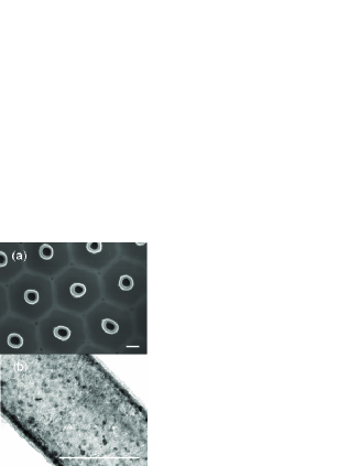
Figure 2: SEM (a) and TEM (b) images for TiO₂/Ni/TiO₂ nanotubes of $180$ nm diameter and a Ni layer thickness of $11-12$ nm. The scale bar indicates in both cases $150$ nm.

Figures 2(a) and (b) present typical SEM and TEM images for TiO₂/Ni/TiO₂ nanotubes with a diameter of around $180$ nm and a Ni layer thickness of $11-12$ nm. Figure 3 shows the hysteresis cycles for three different samples with diameters of $180$, $220$ and $260$ nm; pore length of around $5$ $\mu$m and Ni layer thickness of $11-12$ nm. The measured coercivities for these dimensions are, in all cases, around $200$ Oe ($1$ Oe $=10^{3}/4\pi$ Am^-1), higher than the coercivity of bulk Ni (around $0.7$ Oe for Ni). Chikazumi64

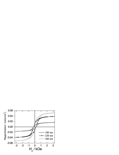
Figure 3: Hysteresis cycles for Ni nanotubes as a function of the tube diameter. The magnetic field is applied parallel to the tube axis. The Ni layer thickness is the same in all cases ($11-12$ nm).

III Model and discussion

III.1 Magnetic field applied parallel to the long axis

As pointed out by Landeros et al. LAE+07 , the curling reversal mode is the dominant magnetization reversal process in magnetic nanotubes. The magnetization curling mode was proposed by Frei et al. FST57 and has been used to investigate the magnetic switching of films IHS+97 and particles with different geometries, like spheres, FST57 prolate ellipsoids FST57 ; ST63 and cylinders. IS89 However, for simplicity, expressions for the nucleation field obtained using infinite cylinders are used.

In the case of a magnetic field applied parallel to the long axis of an infinite tube, we present an analytical approach to the nucleation field obtained from a Ritz model. Calculations are shown in the Appendix and lead us to write

$$\frac{H_{n}^{V}}{M_{0}}=-\frac{2K}{\mu_{0}M_{0}^{2}}-\alpha\left(\beta\right)\frac{L_{ex}^{2}}{R^{2}}\ ,$$ (1)

where $L_{x}=\sqrt{2A/\mu_{0}M_{0}^{2}}$, $M_{0}$ is the saturation magnetization, $A$ is the stiffness constant of the magnetic material, $K$ is the magnetocrystalline anisotropy constant and

$$\alpha\left(\beta\right)=\frac{8}{3}\frac{\left(14-13\beta^{2}+5\beta^{4}\right)}{\left(11+11\beta^{2}-7\beta^{4}+\beta^{6}\right)}\ .$$ (2)

Equation (1) has been previously obtained by Chang et al. CLY94 starting from the Brown’s equations. They obtained $\alpha(\beta)\equiv q^{2}$, with $q$ satisfying

$$\frac{qJ_{0}(q)-J_{1}(q)}{qY_{0}(q)-Y_{1}(q)}-\frac{\beta qJ_{0}(\beta q)-J_{1}(\beta q)}{\beta qY_{0}(\beta q)-Y_{1}(\beta q)}=0\ .$$ (3)

Here $J_{p}\left(z\right)$ and $Y_{p}\left(z\right)$ are Bessel functions of the first and second kind, respectively. Equation (3) has an infinite number of solutions, out of which only the one with the smallest nucleation field has to be considered. Aharoni96 Therefore, the nucleation field depends on $\alpha(\beta)$, which is related to the internal and external radii of the tube. Figure 4 illustrate $\alpha$ as a function of $\beta$, obtained numerically from Brown’s equations, Eq. (3), and by means of Eq. (2) using our analytical approach (Ritz method). We observe that both results are similar, showing a perfect agreement for nanowires $\left(\beta=0\right)$ and very narrow nanotubes $\left(\beta\rightarrow 1\right)$. This behavior lead us to simply use the analytical expression, Eq. (2), to calculate the nucleation field of a magnetic nanotube.

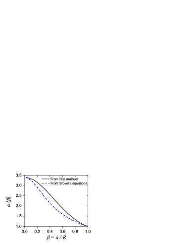
Figure 4: $\alpha$ as a function of $\beta$ from Eq. (3) (dashed line) and by means of our analytical approach, Eq. (2) (solid line).

Therefore, $\alpha(\beta)$ is a decreasing function of the aspect ratio $\beta=a/R$ of the tube. It is clear that, for $\beta=0$, i.e., for an infinite cylinder (or nanowire), $\alpha\left(0\right)=1.08\pi$, as previously calculated by Shtrikman et al. ST63

As pointed by Aharoni, Aharoni97 for a prolate spheroid with $\theta_{0}=0$, a jump of the magnetization at, or near, the curling nucleation field occurs. Therefore, the coercivity is quite close to the absolute value of the nucleation field. Then, we assumed here that $-H_{n}^{V}$ is a good approximation to the coercivity, $H_{c}^{V}$, when the reversal is by curling, as in other works considering infinite cylinders. Ishii91 ; ST63

Now we investigate the validity of Eqs. (1) and (2) by calculating the coercivity for different samples experimentally investigated. Table I summarizes the geometrical parameters of the arrays, measured $H_{c}$, and calculated $H_{c}^{V}$. In our calculations we used $M_{0}=4.85\times 10^{5}$ A/m and $K=4.5\times 10^{3}$ J/m³, both taken from Ref. [22] at room temperature. In the same reference it is pointed that $A$ ranges for any material from $1$ to $2\times 10^{-11}$ J/m. However, by means of field-dependent elastic small-angle neutron scattering (SANS), the exchange-stiffness constant $A$ for Ni was determined by Michels et al. MWW+00 At ambient temperature $A=7.6\pm 0.3\times 10^{-12}$ J/m was reported for nanocrystalline samples while $9.2\pm 0.2\times 10^{-12}$ J/m was obtained at $T=5$ K. For our calculations we choose $A=7.6\times 10^{-12}$ J/m.

Table 1: Parameters for different Ni nanotube arrays with different tube diameters ($2R$) and $5$ $\mu$m tube length. $H_{c}$ represents the experimentally measured coercive field.

$2R\left(nm\right)$	$\beta$	$H_{c}\left(Oe\right)$	$H_{c}^{V}\left(Oe\right)$
$180$	$0.88$	$200$	$231$
$220$	$0.90$	$200$	$215$
$260$	$0.91$	$200$	$206$

In the measured samples, small variations of around $5$ Oe for the coercive field were detected. However, we consider these variations to be within the range of measurement error. From the work of AlMawlawi et al ACM91 small variations of the coercivity are observed for nanowires as a function of the aspect ratio for aspect ratios higher than 20. In order to observe small variations in the coercivity, very well geometrically characterized samples need to be measured with well controlled inter-element interactions. In our samples the center to center distance is fixed, and then the strength of interactions is also different from one sample to other, making a direct comparison difficult. The computed values for the coercivity are larger than the experimental data. We ascribe such differences between calculations and experimental results to the interaction of each tube with the stray field produce by the array. This field originated in the effective antiferromagnetic coupling between neighboring tubes, which reduces the coercive field as previously demonstrated in nanowires. Hertel01 ; BAA+06 As $\beta\rightarrow 1$ the contribution of the stray field diminishes and a better agreement between theory and experiment is obtained. Besides, a fully realistic approach needs to consider a finite nanotube, making much more complex the calculations and the expression for the energy. Therefore, the small discrepancy between experiments and model can be regarded as the result of our models simplification.

III.2 Angular dependence of the coercivity

We now proceed to investigate the angular dependence of the coercivity for magnetic nanotubes. We calculate the coercive field $H_{c}^{k}$ assuming each of the previously mentioned reversal mechanisms, $k=C$ (coherent) or $V$ (curling).

Coherent-mode rotation (C)

The angular dependence of the nucleation for a coherent magnetization reversal was calculated by Stoner-Wohlfarth SW48 and gives

$$\frac{H_{n}^{C}}{M_{0}}=-\frac{1-3N_{z}}{2}\frac{\sqrt{1-t^{2}+t^{4}}}{1+t^{2}}\ ,$$ (4)

where $t=\tan^{\frac{1}{3}}\left(\theta_{0}\right)$ and $N_{z}$ corresponds to the demagnetizing factor of the ellipsoid along $z$. For a tube, the demagnetizing factor can be calculated from Escrig et al. ELA+07 , so that

$$N_{z}=\frac{2R}{L\left(1-\beta^{2}\right)}\int_{0}^{\infty}\frac{dq}{q^{2}}\left(J_{1}\left(q\right)-\beta J_{1}\left(\beta q\right)\right)^{2}\left(1-e^{-q\frac{L}{R}}\right)\ .$$

In the Stoner-Wolhfarth model SW48 the nucleation field, $H_{n}^{C}$, does not represents the coercivity, $H_{c}^{C}$, in all cases. However, from the discussion on p 21 [27], the coercivity can be written as

$$H_{c}^{C}=\left\{\begin{array}[]{c}\left|H_{n}^{C}\right|\quad 0\leq\theta_{0}\leq\pi/4\\ 2\left|H_{n}^{C}\left(\theta_{0}=\pi/4\right)\right|-\left|H_{n}^{C}\right|\quad\pi/4\leq\theta_{0}\leq\pi/2\end{array}\right.\ .$$

Curling-mode rotation (V)

The angular dependence of the curling nucleation field in a finite prolate spheroid was obtained by Aharoni. Aharoni97 By extending the expression for the switching field to take into account the internal radii of tubes, we obtain

$$\frac{H_{n}^{V}}{M_{0}}=\frac{\left(N_{z}-\frac{\alpha\left(\beta\right)L_{x}^{2}}{R^{2}}\right)\left(N_{x}-\frac{\alpha\left(\beta\right)L_{x}^{2}}{R^{2}}\right)}{\sqrt{\left(N_{z}-\frac{\alpha\left(\beta\right)L_{x}^{2}}{R^{2}}\right)^{2}\sin^{2}\theta_{0}+\left(N_{x}-\frac{\alpha\left(\beta\right)L_{x}^{2}}{R^{2}}\right)^{2}\cos^{2}\theta_{0}}}$$ (5)

Figure 5 illustrates the coercive field as a function of $\theta_{0}$ for an infinite nickel nanotube. Dashed curves represent the coercivity of a nanotube due to a reversal curling mode. The cutoff of the curves corresponds to the transition angles, $\theta_{0}^{T}$, at which a coherent reversal mode appears. The most remarkable feature of these curves is that the general shape for nanotubes is similar to the one for nanowires. Differences, of course, are far from being negligible, and the internal radii must be taken into account in any proper analysis of experimental data. For example, using Eq. (5) we found that for a very thin nanotube ($\beta=0.9$) with $R=50$ nm, the coercivity is almost the same as in a nanowire with $R=100$ nm. We also observe in this figure that, for $\theta_{0}>60^{0}$, a small uncertainly in the measurement of $\theta_{0}$ can cause large changes in the coercivity.

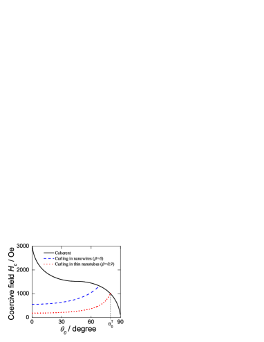
Figure 5: Angular dependence of the coercivity, $H_{c}$, in an infinite nickel nanotube with $R=50$ nm. The solid line represents the coherent rotation, the dashed line corresponds to the curling mode for $\beta=0$, and the dotted line illustrates our results for the curling mode in a tube defined by $\beta=0.9$.

We now investigate the dependence of the coercivity as a function of $R$. We illustrate our results with trajectories of the transition angle, $\theta_{0}^{T}$, in Fig. 6 for Ni. Each line separates the coherent reversal mode (upper) from the curling reversal mode (lower). Results for nickel also represent iron oxide tubes because of the similar magnetic parameters of both materials. In the considered range of parameters, we observe that an increase of the external radii, $R$, or $\beta$ (see Fig. 7) results in an increase of the transition angle, $\theta_{0}^{T}$, enhancing the region of stability of the curling reversal mode. However, the dependence of the coercivity on $R$ is stronger than on $\beta$.

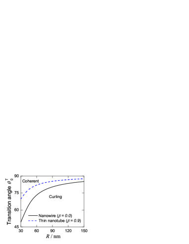
Figure 6: Trajectories of the transition angle, $\theta_{0}^{T}$, as a function of $R$, for $\beta=0$ (solid line) and $\beta=0.9$ (dashed line).

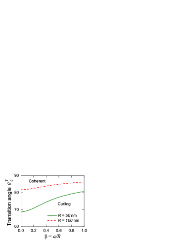
Figure 7: Trajectories of the transition angle, $\theta_{0}^{T}$, as a function of $\beta$, for $R=50$ nm (solid line) and $R=100$ nm (dashed line).

IV Conclusions

In conclusion, by means of theoretical studies and experimental measurements, we have investigated the coercivity in magnetic nanotubes. We have obtained Ni nanotubes by atomic layer deposition into alumina membranes. ALD proves to be a powerful technique, which allows us to have a very precise control of layer growth. We have also derived an analytical expression that allows one to obtain the coercivity when a magnetic field is applied parallel to the tube axis. Good agreement between the measured magnetic properties of Ni nanotubes and theoretical calculations is obtained. Finally, this calculation has been extended to the case of an angular dependence of the coercivity, where a transition from curling-mode rotation to coherent-mode rotation has been observed. However, further experimental work remains to be done in order to observe this transition.

Appendix: nucleation field for an infinite nanotube from a Ritz model

.

We use the term curling mode here not in reference to an eigenfunction of Brown’s equation. In our case we replace the spatial dependence of the curling eigenfunction by a Ritz model that approximates the curling eigenmode, which turns out to be quite simple. We use the Ritz model previously used by Ishii et al. for infinite cylinders. Ishii91 We assume the following model for the magnetization

$$\varepsilon m_{x} = -\varepsilon\left(\frac{r}{R}-\frac{r^{3}}{3R^{3}}\right)\sin\phi$$

$$\varepsilon m_{y} = \varepsilon\left(\frac{r}{R}-\frac{r^{3}}{3R^{3}}\right)\cos\phi$$

$$\varepsilon m_{z} = 1-\frac{\varepsilon^{2}}{2}\left(m_{x}^{2}+m_{y}^{2}\right)\ ,$$

which satisfies $\varepsilon^{2}m_{x}^{2}+\varepsilon^{2}m_{y}^{2}+\varepsilon^{2}m_{z}^{2}=1+\vartheta\left(\varepsilon^{4}\right)$, with $\varepsilon$ an infinitesimal parameter.

The total energy density $E$ is generally given by the sum of four terms corresponding to the magnetostatic $E_{dip}^{V}$, the exchange $E_{ex}^{V}$, the magnetocrystalline anisotropy $E_{K}^{V}$, and the Zeeman $E_{h}^{V}$ (resulting from the interaction between $\mathbf{M}$ and an external field $\mathbf{H}_{a}$), can be calculated using the well known continuum theory of ferromagnetism. Aharoni96 Because in this case we do not have charges in the surface, the contribution from the magnetostatic energy density results equal to zero, $E_{dip}^{V}=0$. The exchange energy density is given by $E_{ex}^{V}=\left(A/s\right)\int\sum\left(\mathbf{\nabla}\varepsilon m_{i}\right)^{2}dv$, with $s=\pi R^{2}\left(1-\beta^{2}\right)$ and $m_{i}=M_{i}/M_{0}$ $\left(i=x,y,z\right)$. Thus, we obtain

$$E_{ex}^{V}=\varepsilon^{2}\frac{\mu_{0}M_{0}^{2}}{27}\left(\frac{L_{x}}{R}\right)^{2}\left(14-13\beta^{2}+5\beta^{4}\right)\ ,$$

The magnetocrystalline anisotropy energy density can be written as $E_{K}^{V}=\left(K/s\right)\int\left(\varepsilon^{2}m_{x}^{2}+\varepsilon^{2}m_{y}^{2}\right)dv$, so that

$$E_{K}^{V}=\varepsilon^{2}\frac{K}{36}\left(11+11\beta^{2}-7\beta^{4}+\beta^{6}\right)\ .$$

Finally we consider the Zeeman energy density, which is given by $E_{h}^{V}=-\left(\mu_{0}H_{a}M_{0}/s\right)\int\varepsilon m_{z}dv$. Thus, we obtain

$$E_{h}^{V}=-\mu_{0}H_{a}M_{0}\left[1-\frac{\varepsilon^{2}}{72}\left(11+11\beta^{2}-7\beta^{4}+\beta^{6}\right)\right]\ .$$

Now we are able to obtain the total energy density $E^{V}$. The second variation in the magnetic energy density $E^{V}$ with respect to a small deviation $\varepsilon\mathbf{m}$ from $\mathbf{\hat{z}}$, where $\mathbf{\hat{z}}$ is the unit vector along the magnetization, must be positive at the equilibrium state and zero at nucleation. Therefore,

$$\frac{H_{n}^{V}}{M_{0}}=-\frac{2K}{\mu_{0}M_{0}^{2}}-\alpha\left(\beta\right)\left(\frac{L_{x}}{R}\right)^{2}\ ,$$

where

$$\alpha\left(\beta\right)=\frac{8}{3}\frac{\left(14-13\beta^{2}+5\beta^{4}\right)}{\left(11+11\beta^{2}-7\beta^{4}+\beta^{6}\right)}\ .$$

References

- (1) S. Iijima, Nature 354, 56 (1991).
- (2) Y. C. Sui, R. Skomski, K. D. Sorge, and D. J. Sellmyer, J. Appl. Phys. 95, 7151 (2004).
- (3) K. Nielsch, F. J. Castano, C. A. Ross, and R. Krishnan, J. Appl. Phys. 98, 034318 (2005).
- (4) Kornelius Nielsch, Fernando J. Castano, Sven Matthias, Woo Lee, and Caroline A. Ross, Adv. Eng. Mater. 7, 217 (2005).
- (5) Z. K. Wang et al., Phys. Rev. Lett. 94, 137208 (2005).
- (6) Feifei Tao, Mingyun Guan, Yuan Jiang, Jianmin Zhu, Zheng Xu, and Ziling Xue, Adv. Mater. 18, 2161 (2006).
- (7) P. Landeros, S. Allende, J. Escrig, E. Salcedo, D. Altbir, and E. E. Vogel, Appl. Phys. Lett. 90, 102501 (2007).
- (8) J. Escrig, P. Landeros, D. Altbir, E. E. Vogel, and P. Vargas, J. Magn. Magn. Mater. 308, 233-237 (2007).
- (9) J. -E. Wegrowe, D. Kelly, A. Franck, S. E. Gilbert, and J. -Ph. Ansermet, Phys. Rev. Lett. 82, 3681 (1999).
- (10) Ke-Hua Zhong, Zhi-Gao Huang, Qian Feng, Li-Qin Jiang, Yan-Min Yang, and Zhi-Gao Cheng, Chin. Phys. Lett. 23, 200 (2006).
- (11) M. Daub, M. Knez, U. Goesele, and K. Nielsch, J. Appl. Phys. 101, 09J111 (2007).
- (12) M. Knez, A. Kadri, C. Wege, U. Goesele, H. Jeske, and K. Nielsch, Nano Lett. 6, 1172 (2006).
- (13) S. Chikazumi, Physics of Magnetism (New York: Wiley, 1964).
- (14) S. E. Frei, S. Shtrikman, and D. Treves, Phys. Rev. 106, 446 (1957).
- (15) Y. Ishii, S. Hasegawa, M. Saito, Y. Tabayashi, Y. Kasajima, and T. Hashimoto, J. Appl. Phys. 82, 3593 (1997).
- (16) S. Shtrikman, and D. Treves in Magnetism, Vol. 3, edited by G. T. Rado and H. Suhl (Academic, New York, London, 1963).
- (17) Y. Ishii, and M. Sato, J. Appl. Phys. 65, 3146 (1989).
- (18) Ching-Ray Chang, C. M. Lee, and Jyh-Shinn Yang, Phys. Rev. B 50, 6461 (1994).
- (19) A. Aharoni Introduction to the Theory of Ferromagnetism (Oxford: Clarendon, 1996).
- (20) A. Aharoni, J. Appl. Phys. 82, 1281 (1997).
- (21) Y. Ishii, J. Appl. Phys. 70, 3765 (1991).
- (22) R. C. O’Handley Modern Magnetic Materials (New York: Wiley, 2000).
- (23) A. Michels, J. Weissmuller, A. Wiedenmann, and J. G. Barker, J. Appl. Phys. 87, 5953-5955 (2000).
- (24) D. AlMawlawi, N. Coombs, and M. Moskovits, J. Appl. Phys. 70, 4421-4425 (1991).
- (25) R. Hertel, J. Appl. Phys. 90, 5752 (2001).
- (26) M. Bahiana, F. S. Amaral, S. Allende, and D. Altbir, Phys. Rev. B 74, 174412 (2006).
- (27) E. C. Stoner, and E. P. Wohlfarth, Philos. Trans. R. Soc. London, Ser. A240, 599 (1948) [Reprinted in IEEE Trans. Magn. 27, 3475 (1991)].