[ To appear in Statistica Sinica]
Nonparametric Conditional Inference for Regression Coefficients with Application to Configural Polysampling

ABSTRACT

We consider inference procedures, conditional on an observed ancillary statistic, for regression coefficients under a linear regression setup where the unknown error distribution is specified nonparametrically. We establish conditional asymptotic normality of the regression coefficient estimators under regularity conditions, and formally justify the approach of plugging in kernel-type density estimators in conditional inference procedures. Simulation results show that the approach yields accurate conditional coverage probabilities when used for constructing confidence intervals. The plug-in approach can be applied in conjunction with configural polysampling to derive robust conditional estimators adaptive to a confrontation of contrasting scenarios. We demonstrate this by investigating the conditional mean squared error of location estimators under various confrontations in a simulation study, which successfully extends configural polysampling to a nonparametric context.
 
Key words and phrases: ancillary; bandwidth; conditional inference; configural polysampling; confrontation; plug-in.

1 Introduction

The classical conditionality principle (Fisher (1934, 1935); Cox and Hinkley (1974)) demands that statistical inference be made relevant to the data at hand by conditioning on ancillary statistics. Arguments for this are best seen from examples in Cox and Hinkley ((1974), Ch.2). Further discussion can be found in Barndorff-Nielsen (1978) and in Lehmann (1981). Under regression models, the ancillary statistic takes the form of studentized residuals. Conditional inference about regression coefficients has been discussed by Fraser (1979), Hinkley (1978), DiCiccio (1988), DiCiccio, Field and Fraser (1990), and Severini (1996), among others. When the error density is completely specified, approximate conditional inference can be made by Monte Carlo simulation or by using numerical integration techniques. The procedure nevertheless becomes computationally intensive if the parameter has a high dimension, in which case large-sample approximations such as those proposed by DiCiccio (1988) and DiCiccio, Field and Fraser (1990) may be necessary. In a nonparametric context where the error density is unspecified, conditional inference has not received much attention despite its clear practical relevance. Fraser (1976) and Severini (1994) tackle the special case of location models. Both suggest plugging in kernel density estimates but provide no theoretical justification for the approach nor any formal suggestion on the choice of bandwidth. The need for sophisticated Monte Carlo or numerical integration techniques endures, and the computational cost is even more expensive than that required by the parametric case. Details of the computational procedures can be found in Severini (1994) and Seifu, Severini and Tanner (1999). In the present paper we prove asymptotic consistency, conditional on the ancillary statistic, of plugging in the kernel density estimator, and derive the orders of bandwidths sufficient for ensuring such consistency. Our proof also suggests a normal approximation to the plug-in approach which is computationally much more efficient for high-dimensional regression estimators.

Consideration of conditionality has motivated different notions of robustness for regression models: see Fraser (1979), Barnard (1981, 1983), Hinkley (1983) and Severini (1992, 1996). Morgenthaler and Tukey (1991) propose a configural polysampling technique for robust conditional inference, which compromises results obtained separately from a confrontation of contrasting error distributions and provides a global perspective for robustness. Our plug-in approach extends configural polysampling to a nonparametric context, substantially broadens the scope of confrontation, and enhances the global nature of the robustness attributed to the resulting inference procedure.

Section 2.1 describes the problem setting. Section 2.2 reviews a bootstrap approach to unconditional inference for regression coefficients. The case of conditional inference is treated in Section 2.3. Section 3 investigates the asymptotics underlying the plug-in approach. Section 4 reviews configural polysampling and extends it to nonparametric confrontations by the plug-in approach. Empirical results are given in Section 5. Section 6 concludes our findings. All proofs are given in the Appendix.

2 Inference for regression coefficients

2.1 Problem setting

Consider a linear regression model $Y_{i}=x_{i}^{\rm T}{\beta}+\tilde{\epsilon}_{i}$, for $i=1,\ldots,n$, where $x_{i}=(x_{i1},\ldots,x_{ip})^{\rm T}$ is the vector of covariates, $\beta=(\beta_{1},\ldots,\beta_{p})^{\rm T}$ is the vector of unknown regression coefficients, and the random errors $\tilde{\epsilon}_{1},\ldots,\tilde{\epsilon}_{n}$ are independent and identically distributed with density $f$ symmetric about 0. Write $Y=(Y_{1},\ldots,Y_{n})^{\rm T}$, $X=[x_{1},\ldots,x_{n}]^{\rm T}$ and $\tilde{\epsilon}=(\tilde{\epsilon}_{1},\ldots,\tilde{\epsilon}_{n})^{\rm T}$. Introduction of a scale parameter leads to a regression-scale model under which $f(u)=f_{0}(u/\sigma)/\sigma$ for an unknown scale $\sigma>0$, and a density $f_{0}$ with unit scale. In this case we have $\tilde{\epsilon}=\sigma\epsilon=\sigma(\epsilon_{1},\ldots,\epsilon_{n})^{\rm T}$, for independent $\epsilon_{1},\ldots,\epsilon_{n}$ distributed with density $f_{0}$, so that $Y=X\beta+\sigma\epsilon$. Throughout the paper we treat $\beta$ as the parameter of interest and $f$, or equivalently, $(\sigma,f_{0})$, as the nuisance parameter of possibly infinite dimension.

Let $\hat{\beta}=\hat{\beta}(Y)$ be a location and scale equivariant estimator of $\beta$ and, under the regression-scale model, $\hat{\sigma}=\hat{\sigma}(Y)$ be a location invariant and scale equivariant estimator of $\sigma$, so that $\hat{\beta}(Xc+dy)=c+d\hat{\beta}(y)$ and $\hat{\sigma}(Xc+dy)=|d|\hat{\sigma}(y)$ for any $(d,c,y)\in{\mathbb{R}}\times{\mathbb{R}}^{p}\times{\mathbb{R}}^{n}$. For example, $\hat{\beta}$ may be the least squares estimator and $\hat{\sigma}^{2}$ the mean squared residuals. Define, for $i=1,\ldots,n$, $\tilde{A}_{i}=Y_{i}-x_{i}^{\rm T}\hat{\beta}$ and $A_{i}=\tilde{A}_{i}/\hat{\sigma}$. We can easily show that $\tilde{A}=(\tilde{A}_{1},\ldots,\tilde{A}_{n})^{\rm T}$ and $A=(A_{1},\ldots,A_{n})^{\rm T}$ provide ancillary statistics under the regression model with known $f$ and the regression-scale model with known $f_{0}$, respectively. When $f_{0}$, and hence $f$, is unspecified, exact conditional inference is not possible as the conditional likelihood of $\beta$ depends in general on $f_{0}$. Adopting Jørgensen’s (1993) notion of I-sufficiency, we see that $A$ is I-sufficient for $f_{0}$, so that any relevant information about $f_{0}$ is contained in $A$. The same applies to $\tilde{A}$ and $f$. Such ancillary-informed knowledge about $f$ and $f_{0}$ forms the basis for nonparametric estimation of the conditional likelihood and facilitates nonparametric conditional inference in an approximate sense.

2.2 Unconditional inference: a bootstrap approach

Under the regression-scale model, the distribution $G_{T}$ of $T=(\hat{\beta}-\beta)/\hat{\sigma}$ does not depend on $(\beta,\sigma)$ and provides a basis for unconditional inference when $f_{0}$ is known. The same applies to the distribution $G_{U}$ of $U=\hat{\beta}-\beta$ under the regression model. Suppose now $f_{0}$, and hence $f$, is unspecified except for symmetry about 0. Under the regression-scale model, we may estimate $G_{T}$ by the residual bootstrap method as follows. Let $F_{n}$ be the empirical distribution of the $2n$ residuals $\pm A_{1},\ldots,\pm A_{n}$. For a random sample $\epsilon^{*}=(\epsilon^{*}_{1},\ldots,\epsilon^{*}_{n})^{\rm T}$ drawn from $F_{n}$, construct a bootstrap resample $Y^{*}=X{\hat{\beta}}+\hat{\sigma}\epsilon^{*}$ and calculate $\hat{\beta}^{*}=\hat{\beta}(Y^{*})$ and $\hat{\sigma}^{*}=\hat{\sigma}(Y^{*})$. The distribution $G_{T}$ is then estimated by the bootstrap distribution, $\hat{G}_{T}$ say, of $(\hat{\beta}^{*}-\hat{\beta})/\hat{\sigma}^{*}$. Under the regression model, we replace $A$ by $\tilde{A}$, calculate $\hat{\beta}^{*}$ from the bootstrap resample $Y^{*}=X{\hat{\beta}}+\epsilon^{*}$ and estimate $G_{U}$ by the bootstrap distribution $\hat{G}_{U}$ of $\hat{\beta}^{*}-\hat{\beta}$.

2.3 Conditional inference: a plug-in approach

Conditional inference about $\beta$ replaces $G_{T}$ and $G_{U}$ used in the unconditional approach by, respectively, the conditional distributions $G_{T|A}(\cdot|a)$ of $T$ given $A=a=(a_{1},\ldots,a_{n})^{\rm T}$ and $G_{U|\tilde{A}}(\cdot|\tilde{a})$ of $U$ given $\tilde{A}=\tilde{a}=(\tilde{a}_{1},\ldots,\tilde{a}_{n})^{\rm T}$.

Consider first the regression-scale model. Define $S=\hat{\sigma}/\sigma$. The conditional joint density of $(S,T)$ given $A=a$ has the expression

$$\kappa(s,t|a)=c_{1}(a)s^{n-1}\prod_{i=1}^{n}f_{0}(s(a_{i}+x_{i}^{T}t)),\mbox{\ \ \ \ }s>0\mbox{\ and \ }t\in\mathbb{R}^{p},$$ (1)

where $c_{1}(a)$ is a normalizing constant depending on $a$. Denote by $g_{T|A}(\cdot|a)$ the conditional density of $T$ given $A=a$. Then, for $t\in{\mathbb{R}}^{p}$ and ${\cal T}\subset{\mathbb{R}}^{p}$, the integrals $g_{T|A}(t|a)=\int_{0}^{\infty}\!\!\!\kappa(s,t|a)\,ds$ and $G_{T|A}({\cal T}|a)=\int_{t\in{\cal T}}g_{T|A}(t|a)\,dt$ can be approximated by either Monte Carlo or numerical integration if $f_{0}$ is known, with increasing computational cost as $p$ increases. When $f_{0}$ is unspecified, we note I-sufficiency of $A$ for $f_{0}$ and propose estimating $f_{0}$ by a kernel density estimate based on $a$: $\hat{f}_{h}(z|a)=(nh)^{-1}\sum_{i=1}^{n}k\left((z-a_{i})/h\right)$, where $k$ is a kernel function and $h>0$ is the bandwidth. This leads to nonparametric estimates $\hat{G}_{T|A}$ and $\hat{g}_{T|A}$ of $G_{T|A}$ and $g_{T|A}$ respectively, which can again be approximated by either Monte Carlo or numerical integration methods. We term this the “plug-in” (PI) approach to distinguish it from the “residual bootstrap” (RB) approach introduced earlier to unconditional inference. The use of studentized residuals $a$ in its derivation guarantees that $\hat{f}_{h}(z|a)$ has unit scale asymptotically. Under symmetry of $f_{0}$, it might be beneficial in practice to use in place of $\hat{f}_{h}$ its symmetrized version, $\tilde{f}_{h}(z|a)=(\hat{f}_{h}(z|a)+\hat{f}_{h}(-z|a))/2$.

Under the regression model, the distribution and density of $U$ conditional on $\tilde{A}=\tilde{a}$ are given, for ${\cal U}\subset{\mathbb{R}}^{p}$ and $u\in{\mathbb{R}}^{p}$, by $G_{U|\tilde{A}}({\cal U}|\tilde{a})=\int_{u\in{\cal U}}g_{U|\tilde{A}}(u|\tilde{a})\,du$ and $g_{U|\tilde{A}}(u|\tilde{a})=c_{3}(\tilde{a})\prod_{i=1}^{n}f(\tilde{a}_{i}+x_{i}^{\rm T}u)$ respectively, for some constant $c_{3}(\tilde{a})$. If $f$ is unspecified, the PI approach substitutes $f$ by $\hat{f}_{h}(\cdot|\tilde{a})$ or $\tilde{f}_{h}(\cdot|\tilde{a})$ to yield plug-in estimates $\hat{G}_{U|\tilde{A}}$ and $\hat{g}_{U|\tilde{A}}$, on which conditional inference can be based.

3 Theory

We consider first the asymptotic behaviour of $G_{T|A}$ and $G_{U|\tilde{A}}$, and then assess the PI approach by substituting kernel estimates for $f$ and $f_{0}$. Take $\ell_{0}\equiv\log f_{0}$ and $\ell\equiv\log f$ and assume the following regularity conditions.

1. $f_{0}$ is symmetric about 0 and positive on $[-C,C]$ for some $C>0$.

2. $f_{0}$ has uniformly bounded continuous derivatives up to order 3, with $f_{0}^{\prime\prime\prime}$ being Lipschitz continuous.

3. ${\mathbb{E}}\,\varepsilon^{2}$, ${\mathbb{E}}\,\varepsilon^{2}\ell_{0}^{\prime}(\varepsilon)^{2}$, ${\mathbb{E}}\,\varepsilon^{2}\ell_{0}^{\prime\prime}(\varepsilon)^{2}$ and ${\mathbb{E}}\,|\varepsilon^{3}\ell_{0}^{\prime\prime\prime}(\varepsilon)|$ are finite for $\varepsilon\sim f_{0}$.

We assume that $X=X_{n}=[x_{n,1},\ldots,x_{n,n}]^{\rm T}$ depends on $n$ and satisfies the following.

1. $X_{n}^{\rm T}X_{n}$ is positive definite for all $n$, and $\Sigma\equiv\lim_{n\rightarrow\infty}n^{-1}X_{n}^{\rm T}X_{n}$ exists and is positive definite.

2. (Generalized Noether condition) $\displaystyle\lim_{n\rightarrow\infty}\max_{1\leq i\leq n}\left\{{x_{n,i}}^{\rm T}(X_{n}^{\rm T}X_{n})^{-1}x_{n,i}\right\}=0$.

3. $\sup_{n}\left\{n^{-1}\sum_{i=1}^{n}({x_{n,i}}^{\rm T}x_{n,i})^{1+\eta}\right\}<\infty$ for some $\eta>0$.

Note that (C1) and (C2) imply asymptotic normality of least squares estimators of $\beta$: see Sen and Singer ((1993), Section 7.2). The location model provides a trivial example that satisfies (C1)–(C3). The following theorem derives the asymptotic conditional distributions of $n^{1/2}T$ and $n^{1/2}U$.

Theorem 1

Assume (C1)–(C3), (D1)–(D3) and that $\hat{\beta}=\beta+O_{p}(n^{-1/2})$ and $\hat{\sigma}=\sigma+O_{p}(n^{-1/2})$. Then

• under the regression-scale model, ${\cal I}^{1/2}(n^{1/2}T-{\cal I}^{-1}\theta)$ is standard normal conditional on $A$, up to order $O_{p}(n^{-1/2})$, where ${\cal I}=n^{-2}X_{n}^{\rm T}X_{n}\sum_{i=1}^{n}\ell_{0}^{\prime}(A_{i})^{2}$ and $\theta=n^{-1/2}\sum_{i=1}^{n}x_{n,i}\ell_{0}^{\prime}(A_{i})$;

• under the regression model, $\tilde{\cal I}^{1/2}(n^{1/2}U-\tilde{\cal I}^{-1}\tilde{\theta})$ is standard normal conditional on $\tilde{A}$, up to order $O_{p}(n^{-1/2})$, where $\tilde{\cal I}=n^{-2}X_{n}^{\rm T}X_{n}\sum_{i=1}^{n}\ell^{\prime}(\tilde{A}_{i})^{2}$ and $\tilde{\theta}=n^{-1/2}\sum_{i=1}^{n}x_{n,i}\ell^{\prime}(\tilde{A}_{i})$.

We see from Theorem 1 that the conditional distributions of $n^{1/2}T$ and $n^{1/2}U$ admit normal approximations with conditional means and covariance matrices depending on the score functions $\ell^{\prime}_{0}$ and $\ell^{\prime}$. The proof of Theorem 1 suggests that the conditional covariance matrices ${\cal I}^{-1}$ and $\tilde{\cal I}^{-1}$ equal, up to order $O_{p}(n^{-1/2})$, the deterministic matrices $I^{-1}$ and $\tilde{I}^{-1}$, where $I=n^{-1}X_{n}^{\rm T}X_{n}\int(\ell^{\prime}_{0})^{2}f_{0}$ and $\tilde{I}=n^{-1}X_{n}^{\rm T}X_{n}\int(\ell^{\prime})^{2}f$, whereas the conditional means ${\cal I}^{-1}\theta$ and $\tilde{\cal I}^{-1}\tilde{\theta}$ have asymptotic unconditional distributions $N(0,I^{-1})$ and $N(0,\tilde{I}^{-1})$, respectively. It follows that exact unconditional inference about $\beta$ may not be correct, not even to first order asymptotically, conditional on the ancillary residuals. For example, an unconditionally exact level $1-\alpha$ confidence set derived from $G_{T}$ has conditional coverage converging in probability to the random limit $\Phi_{I^{-1}}(\Theta_{1-\alpha}-Z)$ for $Z\sim N(0,I^{-1})$, where $\Phi_{\Lambda}$ denotes the $p$-variate $N(0,\Lambda)$ distribution and $\Phi_{\cal K}(\Theta_{1-\alpha})=1-\alpha$ for some covariance matrix ${\cal K}$. The only exception is when $\hat{\beta}$ is the exact maximum likelihood estimator of $\beta$.

To validate the PI approach asymptotically, we assume that the kernel function $k$ satisfies the following.

1. $k$ has support $[-c,c]$, for some $c>0$, and is symmetric about 0.

2. $k$ is twice differentiable with $k^{\prime\prime}$ being Lipschitz continuous.

3. there exists some $q\geq 2$ such that $\int k=1$, $\int u^{j}k(u)\,du=0$ for $j=1,\ldots,q-1$, and $\int u^{q}k(u)\,du\neq 0$.

First-order approximation of the PI approach amounts to substitution of $\hat{f}_{h}(\cdot|A)$ or $\tilde{f}_{h}(\cdot|A)$ for $f_{0}$ in the score $\ell^{\prime}_{0}$ that defines the conditional normal mean ${\cal I}^{-1}\theta$ and covariance matrix ${\cal I}^{-1}$ of $n^{1/2}T$. We consider a slightly different score estimator in the theoretical development below. This simplifies the proof and is asymptotically equivalent to the original PI proposal. Denote by $A_{-i}$ the ancillary statistic $A$ with $A_{i}$ excluded, for $i=1,\ldots,n$. Define, for $i=1,\ldots,n$ and $m=0,1,\ldots\>$, the “leave-one-out” kernel estimator of $f_{0}^{(m)}$ by $\hat{f}^{(m)}_{h}(z|A_{-i})=((n-1)h^{m+1})^{-1}\sum_{j\not=i}k^{(m)}((z-A_{j})/h)$. Symmetry of $f_{0}$ motivates an anti-symmetrized leave-one-out estimate of $\ell_{0}^{\prime}(A_{i})$ given by

$$\hat{\ell}^{\prime}_{h_{0},h_{1}}(A_{i}|A_{-i})=2^{-1}\left\{\hat{f}^{\prime}_{h_{1}}(A_{i}|A_{-i})/\hat{f}_{h_{0}}(A_{i}|A_{-i})-\hat{f}^{\prime}_{h_{1}}(-A_{i}|A_{-i})/\hat{f}_{h_{0}}(-A_{i}|A_{-i})\right\},$$

for bandwidths $h_{0},h_{1}>0$. This leads to estimators of $\theta$ and ${\cal I}$, given by $\theta^{\dagger}=n^{-1/2}\sum_{i=1}^{n}x_{n,i}\hat{\ell}^{\prime}_{h_{0},h_{1}}(A_{i}|A_{-i})$ and ${\cal I}^{\dagger}=n^{-2}X_{n}^{\rm T}X_{n}\sum_{i=1}^{n}\hat{\ell}^{\prime}_{h_{0},h_{1}}(A_{i}|A_{-i})^{2}$, respectively. Similar steps lead to estimates $\tilde{\theta}^{\dagger}$ and $\tilde{\cal I}^{\dagger}$ of $\tilde{\theta}$ and $\tilde{\cal I}$, respectively, under the regression model. The following theorem concerns consistency of the above estimators.

Theorem 2

Assume (K1)–(K3), the conditions in Theorem 1 and that $h_{m}\rightarrow 0$ and $nh_{m}^{2m+3}\rightarrow\infty$, $m=0,1$. Then

• under the regression-scale model, ${\cal I}^{\dagger}={\cal I}+O_{p}(\delta_{1})={\cal I}+o_{p}(1)$ and $\theta^{\dagger}=\theta+O_{p}(\delta_{2})=\theta+o_{p}(1)$;

• under the regression model, $\tilde{\cal I}^{\dagger}=\tilde{\cal I}+O_{p}(\delta_{1})=\tilde{\cal I}+o_{p}(1)$ and $\tilde{\theta}^{\dagger}=\tilde{\theta}+O_{p}(\delta_{2})=\tilde{\theta}+o_{p}(1)$,

where $\delta_{1}=h_{0}^{q}+h_{1}^{q}+n^{-1/2}(h_{0}^{-1/2}+h_{1}^{-3/2})$ and $\delta_{2}=h_{0}^{q}+h_{1}^{q}+n^{-1/2}(h_{0}^{-3/2}+h_{1}^{-5/2})$.

Theorems 1 and 2 together justify the PI approach asymptotically and derive the valid orders of the bandwidths involved. Note that the conditional distributions of $n^{1/2}T$ and $n^{1/2}U$ can be estimated consistently by $N({\cal I}^{\dagger-1}\theta^{\dagger},{\cal I}^{\dagger-1})$ and $N(\tilde{\cal I}^{\dagger-1}\tilde{\theta}^{\dagger},\tilde{\cal I}^{\dagger-1})$, respectively, provided that $h_{0},h_{1}\rightarrow 0$ and $nh_{0}^{3},nh_{1}^{5}\rightarrow\infty$. We term this the “normal approximate plug-in” (NPI) approach to distinguish it from the PI approach which directly simulates from, or numerically evaluates, $\hat{G}_{T|A}$ and $\hat{G}_{U|\tilde{A}}$. The normal approximation error can be kept to a minimum of order $O_{p}(n^{-q/(5+2q)})$ by setting $h_{1}\propto n^{-1/(5+2q)}$, $h_{0}=O(n^{-1/(5+2q)})$ and $h_{0}^{-1}=O(n^{5/(15+6q)})$. Park (1993) introduced trimming constants to the estimated score $\hat{\ell}_{h_{0},h_{1}}^{\prime}$ to correct for its occasional erratic behaviour.

Remark. Adaptive estimation constructs asymptotically efficient estimators by substituting nonparametric score estimates in a one-step maximum likelihood approximation. Stone (1975) considered adaptive estimation under the symmetric location model. Bickel (1982) extended the construction to linear models. Under our regression setup, the adaptive estimator built upon an equivariant regression estimator has conditional and unconditional distributions equivalent to first order, and can be viewed as an equivariant regression estimator with conditional mean recentered at the true regression parameter. This connection implies asymptotic equivalence of adaptive estimation and the NPI approach, suggesting that the latter can be approximated by unconditional inference based on adaptive estimators. Many nonparametric methods, such as the bootstrap, that are intended mainly for unconditional inference are readily available for estimation of such unconditional distributions.

4 Robustness and configural polysampling

Morgenthaler and Tukey (1991) suggest a global, finite-sample, notion of robustness that pays due attention to ancillarity. Their method, known as configural polysampling, makes robust inference by conditioning on an ancillary configuration of the observed data under a confrontation of rival parametric models. Its dissociation from asymptotic reasoning makes the method attractive for finite samples and distinct from such conventional devices as the influence function and the breakdown point. Morgenthaler (1993) specializes it to linear models and develops computationally simple procedures for robust estimation.

A key ingredient to configural polysampling is the choice of a confrontation pair $(\cal F,G)$, where $\cal F$ and $\cal G$ denote extremes, in a spectrum of error distributions of practical interest, under which inference is done separately and the resulting analyses combined in an optimal way. The approach can be generalized to deal with more than two distributions in the confrontation. Morgenthaler and Tukey (1991) suggest taking $\cal F$ and $\cal G$ to be the normal and slash distributions to encompass a spectrum ranging from light- to heavy-tailed distributions. To fix ideas, consider estimation of $\beta$ by an equivariant estimator $V$, such that $V(Y)=\hat{\beta}+\hat{\sigma}V(A)$. When $f_{0}={\cal F}$, the conditional mean squared error (cMSE) of $V$ given $A$ is minimized at $V(A)=V_{\cal F}(A)\equiv-\mathbb{E}_{\cal F}[S^{2}T|A]/\mathbb{E}_{\cal F}[S^{2}|A]$, leading to Pitman’s (1939) famous estimator, an early example of optimal estimation driven by the conditionality principle. Thus we may write, for an arbitrary equivariant estimator $V$, $\mbox{cMSE}_{\cal F}(V|A)=\mbox{cMSE}_{\cal F}(V_{\cal F}|A)+\sigma^{2}\mathbb{E}_{\cal F}[S^{2}|A](V(A)-V_{\cal F}(A))^{2}$. Morgenthaler and Tukey (1991) select a “bioptimal” $V$ by minimizing $P_{\cal F}\times\mbox{cMSE}_{\cal F}(V|A)+P_{\cal G}\times\mbox{cMSE}_{\cal G}(V|A)$, for a pair of shadow prices $P_{\cal F}$ and $P_{\cal G}$. Alternatively, a minimax estimator $V$ of $\beta$ can be obtained by minimizing the maximum of $\mbox{cMSE}_{\cal F}(V|A)$ and $\mbox{cMSE}_{\cal G}(V|A)$, which often amounts to solving the equation $\mbox{cMSE}_{\cal F}(V|A)=\mbox{cMSE}_{\cal G}(V|A)$. The regression model can be treated similarly. In confidence interval problems one may, for example, minimize the conditional mean interval length subject to correct unconditional coverages under $\cal F$ and $\cal G$. In general, configural polysampling fine-tunes statistical procedures to achieve simultaneous efficiency over a spectrum of distributions determined by $(\cal F,\cal G)$. It can be generalized with data-driven choices of $(\cal F,\cal G)$, thereby robustifying the inference procedure in a global sense. We envisage confrontations $(\cal F,\cal G)$ which reflect practical concerns in robust statistical inference. For example, we may confront parametric with nonparametric approaches, unconditional with conditional approaches, asymptotic approximation with finite-sample methods, small with large bandwidths in any kernel-based approach, or any two competing nonparametric approaches. In these possible confrontations, our PI or NPI approaches can play a prominent role in robustifying the inference outcome specific to the observed ancillary configuration. Further empirical evidence is presented in Section 5.2.

5 Empirical studies

5.1 Confidence intervals

Our first study compared the conditional coverage probabilities of the PI and NPI intervals with those of the exact unconditional and RB intervals. We considered the location model with $p=1$ and $\beta=1$, and took $f$ to be the Student’s $t_{5}$ density, which satisfies (D1)–(D3). The “conditional” samples, all subject to a common observed value of $\tilde{A}$, were obtained by rejection sampling. Three sample sizes, $n=15$, 30 and 100, were considered. The nominal level $1-\alpha$ was chosen to be $0.90,0.91,\ldots,0.99$. Each conditional coverage was estimated from 5000 “conditional” samples. Construction of the PI and NPI intervals was based on 5000 samples drawn from $\hat{G}_{U|\tilde{A}}$ and its normal approximation, respectively. The RB interval was based on 1000 bootstrap samples and the exact unconditional interval on 5000 samples drawn from $f$ itself. The kernel function $k$ was taken to be the standard normal density.

The objective of this study is to demonstrate the importance of conditioning and the effectiveness of PI and NPI in constructing conditional confidence intervals. Despite its importance in practice, the issue of bandwidth selection is not our main interest and we set $h=1$ throughout the study, the best choice in a pilot study done on four different sets of ancillary residuals. Conventional methods for practical bandwidth selection include the normal referencing rule, cross-validation and the (conditional) bootstrap. Alternatively, an innovative approach can be based on configural polysampling under a confrontation of two extreme choices of bandwidth. This will be illustrated in Section 5.2. For the NPI approach we used the true $f$, rather than its kernel estimate, for computing $\ell^{\prime}$ in order to examine the effects on conditional coverages due exclusively to normal approximation.

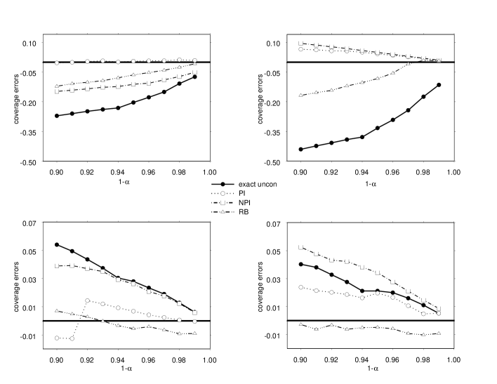
Figure 1: Conditional coverage errors of exact unconditional, PI, NPI and RB intervals, for $n=15$.

Figure 1 plots the conditional coverage errors against $1-\alpha$ for $n=15$ for four different sets of $\tilde{A}$, chosen specifically such that the exact unconditional intervals undercover in two cases and overcover in the other two. We see that the exact unconditional interval has very large conditional coverage error compared to the two plug-in approaches, except for the fourth case where it outperforms the NPI approach. Surprisingly, the RB interval yields more accurate coverage than does the exact unconditional interval, although the former is designed primarily for estimating the latter. It is evident that $U$ has very different unconditional and conditional distributions given our choices of $\tilde{A}$. The PI approach works effectively for all four choices of $\tilde{A}$. Inferior in general to the PI intervals, NPI nevertheless corrects the exact unconditional interval to some extent, although the correction is less remarkable when the unconditional interval overcovers. Similar conclusions are observed for $n=30$ and 100. We also investigated choices of $\tilde{A}$ given which the exact unconditional interval is conditionally accurate. The results, not shown in this report, suggest that both the PI and NPI intervals remain, as expected, accurate in those cases.

5.2 Robust conditional estimation

The second study illustrates applications of the PI approach in configural polysampling procedures for robust conditional inference. We considered three types of confrontation pairs, all reflecting genuine practical concerns: (i) the normal versus the slash distributions; (ii) the least squares method versus the PI approach based on bandwidth $h=Cn^{-1/9}$, a multiple of the optimal order; and (iii) the PI approach based on contrasting bandwidths $h_{a}$ and $h_{b}$. Note that (i) was conceived by Morgenthaler and Tukey (1991) for achieving robustness across symmetric, unimodal, distributions of different tail behaviour. Case (ii) contrasts conditional with unconditional inferences. Case (iii) suggests a practical robust solution, which respects the conditionality principle, to the problem of bandwidth selection in the PI method. In the study we set $C=0.1,0.5,1.0,1.5,2.0,2.5$ and $h_{a}=0.1,h_{b}=2.0$. The kernel $k$ was taken to be the standard normal density.

We considered again a location model and compared the mean squared error of minimax location estimates obtained under different confrontations. The least squares estimate, the sample mean, was also included for comparison. Given a fixed set of residuals, we generated 100,000 “conditional” random samples of sizes $n=15$ and $30$ from each of six different distributions: the Student’s $t_{1}$, the normal mixture $\frac{1}{2}N(-3,1)+\frac{1}{2}N(3,1)$ and the centered beta distributions with support $[-5,5]$ and shape parameters $(1/2,1/2),(2,2),(1/2,2)$ and $(2,1/2)$, among which the $t_{1}$ and $\beta(2,2)$ densities have bell-like shapes and can be deemed to lie within the normal-slash spectrum. We are here not so much concerned with asymptotic validity as interested in robustness against model departures in a broad context. Indeed, all six distributions except the normal mixture fail to satisfy (D3).

Table 1 reports the cMSE’s of the various estimates, obtained by averaging over the conditional samples generated from each distribution. We see that confrontation types (ii) and (iii) give remarkably small cMSE compared to (i), which is even less accurate than the unconditional least squares estimate under distributions outside the normal-slash spectrum. Confrontation type (ii) outperforms (i) under all choices of $C$ and most of the underlying distributions except $t_{1}$, under which use of large $C$ in (ii) gives results comparable to (i). Particularly encouraging are the results obtained using confrontation (iii), which returns an accurate, robustified PI estimate for which the bandwidth is implicitly selected from candidate values lying between $h_{a}$ and $h_{b}$.

5.3 A real data example

DiCiccio (1988) and Sprott (1980, 1982) made conditional inference about a real location parameter $\beta$ by fitting a location-scale model with $t_{\lambda}$ error to Darwin’s data (Fisher (1960), P.37) on 15 height differences between cross- and self-fertilized plants. We removed the $t_{\lambda}$ assumption, set $\hat{\beta}$ to be (I) the sample mean and (II) the sample median, both being location equivariant, and constructed $95\%$ two-sided RB, PI and NPI intervals for $\beta$ in both cases. The RB interval was based on 50,000 bootstrap samples. The NPI interval was built on the anti-symmetrized leave-one-out score estimate, for which the bandwidths $h_{0}$ and $h_{1}$ were fixed to be (give the actual number, not formula) using the normal referencing rule.

For (I), we calculated the RB and NPI intervals to be $(2.46,39.43)$ and $(8.78,40.80)$, respectively, and the PI intervals to be $(17.51,24.45)$, $(11.33,35.84)$, $(10.42,39.12)$, $(8.38,42.15)$, $(4.86,44.44)$ and $(2.24,45.51)$ based on bandwidths $h=mh_{0}$, for $m=0.2,0.5,0.7,1.0,1.3,1.5$, respectively. The results are in agreement with DiCiccio’s (1988) and Sprott’s (1980, 1982) findings, suggesting plausibility of their Student’s $t$ error assumption. The case (II) gives similar results except that the endpoints are shifted slightly to the right, in general.

6 Conclusion

We establish consistency of the PI approach to conditional inference and derive sufficient bandwidth orders. The NPI approach provides a computationally convenient normal approximation to it. Effectiveness of the approaches is confirmed by empirical findings. The computational cost of PI depends on the dimension $p$ and the efficiency with which we can simulate from $\hat{g}_{T|A}$ or $\hat{g}_{U|\tilde{A}}$. The computing times for both plug-in approaches were found to be within seconds under the location model considered in Section 5.1.

Incorporation of the plug-in approaches into confrontations extends configural polysampling to the nonparametric realm, rendering the resulting conditional inference an extra dimension of robustness. When applied to a confrontation of two extreme bandwidths, the technique suggests an innovative solution, which observes the conditionality principle, to bandwidth selection in practical applications of the PI approaches. We remark that confrontations of more than two specifications of error density can be considered in configural polysampling to further robustify the inference outcome, although then the minimax algorithm is necessarily more computationally involved.

7 Appendix

7.1 Proof of Theorem 1

Under the regression-scale model, we deduce, by a Taylor expansion of (1) in powers of $n^{-1/2}$, that the density of $n^{1/2}(\log S,T)$ conditional on $A$ is proportional, up to $O_{p}(n^{-1/2})$, to the product of the $N({\cal J}^{-1}\psi,{\cal J}^{-1})$ and $N({\cal I}^{-1}\theta,{\cal I}^{-1})$ density functions, where ${\cal J}=-\,n^{-1}\sum_{i=1}^{n}\left\{A_{i}\ell_{0}^{\prime}(A_{i})+A_{i}^{2}\ell_{0}^{\prime\prime}(A_{i})\right\}$ and $\psi=n^{-1/2}\sum_{i=1}^{n}\left(A_{i}\ell_{0}^{\prime}(A_{i})+1\right)$. This proves part (i). Part (ii) follows by similar, but simpler arguments.

7.2 Proof of Theorem 2

Note that Linton and Xiao’s (2001) Lemma 2 can be adapted to deduce that

$$\hat{f}_{h}^{(m)}(\pm A_{i}|A_{-i})=f^{(m)}_{0}(\pm A_{i})+O_{p}(h^{q}+n^{-1/2}h^{-m-1/2}),\;\;m=0,1,$$ (2)

uniformly in $i\in\{1,\ldots,n\}$. It follows that $\hat{\ell}^{\prime}_{h_{0},h_{1}}(A_{i}|A_{-i})=\ell^{\prime}_{0}(A_{i})+O_{p}(\delta_{1})$, and hence the result for ${\cal I}^{\dagger}$.

Define $\delta^{\pm}_{im}=\pm\left\{\hat{f}_{h_{m}}^{(m)}(\pm\epsilon_{i}|A_{-i})-\hat{f}_{h_{m}}^{(m)}(\pm A_{i}|A_{-i})\right\}$. That $\hat{\beta}$ and $\hat{\sigma}$ are $n^{1/2}$-consistent implies that $\mu\equiv\log(\hat{\sigma}/\sigma)$ and $\tau\equiv\hat{\beta}/\hat{\sigma}-\beta/\sigma$ are both $O_{p}(n^{-1/2})$. Write $\bar{x}=\sum_{i=1}^{n}x_{n,i}/n$. Conditioning on $\epsilon_{i}$, standard asymptotic theory yields

$$(n-1)^{-1}h_{m}^{-m-2}\sum_{j\neq i}k^{(m+1)}((\pm\epsilon_{i}-\epsilon_{j})/h_{m})(\pm x_{n,i}-x_{n,j})$$

$$= f^{(m+1)}_{0}(\pm\epsilon_{i})(\pm x_{n,i}-\bar{x})+O_{p}(h_{m}^{q}+n^{-1/2}h_{m}^{-m-3/2}),$$

$$(n-1)^{-1}h_{m}^{-m-2}\sum_{j\neq i}k^{(m+1)}((\pm\epsilon_{i}-\epsilon_{j})/h_{m})(\pm\epsilon_{i}-\epsilon_{j})$$

$$= -\,(m+1)f^{(m)}_{0}(\pm\epsilon_{i})+O_{p}(h_{m}^{q}+n^{-1/2}h_{m}^{-m-1/2}),$$

so that

$$\delta^{\pm}_{im} = \pm f_{0}^{(m+1)}(\pm\epsilon_{i})(\pm x_{n,i}-\bar{x})^{\rm T}(\tau+\mu\beta/\sigma)\mp(m+1)\mu f_{0}^{(m)}(\pm\epsilon_{i})$$ (3)

$$\mbox{\ \hskip 85.35826pt}+O_{p}(n^{-1/2}h_{m}^{q}+n^{-1}h_{m}^{-m-3/2}).$$

Noting (3), and that (2) also holds if $\pm A_{i}$ is replaced by $\pm\epsilon_{i}$, we have

$$\hat{\ell}^{\prime}_{h_{0},h_{1}}(A_{i}|A_{-i})$$ (4)

$$= \hat{f}^{\prime}_{h_{1}}(\epsilon_{i}|A_{-i})/\hat{f}_{h_{0}}(\epsilon_{i}|A_{-i})-\left[f^{\prime\prime}_{0}(\epsilon_{i})x_{n,i}^{\rm T}(\tau+\mu\beta/\sigma)-2\mu f^{\prime}_{0}(\epsilon_{i})\right]/f_{0}(\epsilon_{i})$$

$$+\left[f^{\prime}_{0}(\epsilon_{i})x_{n,i}^{\rm T}(\tau+\mu\beta/\sigma)-\mu f_{0}(\epsilon_{i})\right]f^{\prime}_{0}(\epsilon_{i})/f_{0}(\epsilon_{i})^{2}+O_{p}\left(n^{-1/2}\delta_{2}\right).$$

Expanding $A_{i}$ about $\epsilon_{i}$, we have

$$\ell^{\prime}_{0}(A_{i}) = f^{\prime}_{0}(\epsilon_{i})/f_{0}(\epsilon_{i})-\left[x_{n,i}^{\rm T}(\tau+\mu\beta/\sigma)+\mu\epsilon_{i}\right]f^{\prime\prime}_{0}(\epsilon_{i})/f_{0}(\epsilon_{i})$$ (5)

$$+\left[x_{n,i}^{\rm T}(\tau+\mu\beta/\sigma)+\mu\epsilon_{i}\right]f^{\prime}_{0}(\epsilon_{i})^{2}/f_{0}(\epsilon_{i})^{2}+O_{p}(n^{-1}).$$

Symmetry of $f_{0}$ and (D3) together imply that $n^{-1/2}\sum_{i=1}^{n}x_{n,i}f^{\prime}_{0}(\epsilon_{i})/f_{0}(\epsilon_{i})$, $n^{-1/2}\sum_{i=1}^{n}x_{n,i}\epsilon_{i}f^{\prime\prime}_{0}(\epsilon_{i})/f_{0}(\epsilon_{i})$, and $n^{-1/2}\sum_{i=1}^{n}x_{n,i}\epsilon_{i}f^{\prime}_{0}(\epsilon_{i})^{2}/f_{0}(\epsilon_{i})^{2}$ are all of order $O_{p}(1)$. It then follows from (4) and (5) that

$$\theta^{\dagger}-\theta=n^{-1/2}\sum_{i=1}^{n}x_{n,i}\left\{\hat{f}^{\prime}_{h_{1}}(\epsilon_{i}|A_{-i})/\hat{f}_{h_{0}}(\epsilon_{i}|A_{-i})-f^{\prime}_{0}(\epsilon_{i})/f_{0}(\epsilon_{i})\right\}+O_{p}(\delta_{2}).$$ (6)

The proof of Linton and Xiao’s (2001) Theorem 1 can be adapted to show that the first term in (6) has order $O_{p}(\delta_{1})$, which can be absorbed into $O_{p}(\delta_{2})$. This completes the proof of (i). Part (ii) follows by similar arguments.

Table 1: Conditional mean squared errors of least squares estimates (LS) and minimax estimates obtained under confrontations (i) normal vs slash, (ii) LS vs PI, (iii) $h_{a}=0.1$ vs $h_{b}=2.0$ in PI.

		Error distribution
		centred	centred	centred	centred		$\frac{1}{2}N(-3,1)$
Confrontation		$\beta(1/2,1/2)$	$\beta(2,2)$	$\beta(1/2,2)$	$\beta(2,1/2)$	$t_{1}$	$+\frac{1}{2}N(3,1)$
$n=15$
(i)	normal vs slash	4.3403	0.6814	1.5399	1.5743	0.5745	2.7075
(ii)	LS vs PI ($C=0.1$)	1.3105	0.4174	0.7947	0.7979	2.0863	1.0709
(ii)	LS vs PI ($C=0.5$)	1.2326	0.4174	0.9643	0.9674	2.0863	0.4513
(ii)	LS vs PI ($C=1.0$)	0.4206	0.3869	1.3331	1.3352	0.9975	0.4351
(ii)	LS vs PI ($C=1.5$)	0.2234	0.3790	1.4512	1.4540	0.7163	0.3631
(ii)	LS vs PI ($C=2.0$)	0.1995	0.3889	1.5092	1.5118	0.6033	0.3921
(ii)	LS vs PI ($C=2.5$)	0.2952	0.4017	1.1576	1.1633	0.5335	0.5787
(iii)	$h_{a}=0.1$ vs $h_{b}=2.0$	0.3508	0.4057	1.0683	1.0670	0.4664	0.6532
	LS	1.3126	0.4178	0.7963	0.7963	2.0837	1.0691
$n=30$
(i)	normal vs slash	1.6922	0.3884	0.3200	0.3216	0.5380	4.4011
(ii)	LS vs PI ($C=0.1$)	0.2277	0.1946	0.0386	0.0391	1.9589	1.9654
(ii)	LS vs PI ($C=0.5$)	0.1068	0.1796	0.0386	0.0391	1.9589	1.9654
(ii)	LS vs PI ($C=1.0$)	0.0116	0.1828	0.0171	0.0169	1.2311	1.2539
(ii)	LS vs PI ($C=1.5$)	0.0049	0.1801	0.0125	0.0120	0.8892	1.0360
(ii)	LS vs PI ($C=2.0$)	0.0010	0.1801	0.0187	0.0189	0.7061	0.9042
(ii)	LS vs PI ($C=2.5$)	0.0071	0.1834	0.0276	0.0279	0.6188	0.9591
(iii)	$h_{a}=0.1$ vs $h_{b}=2.0$	0.0186	0.1867	0.0321	0.0328	0.5566	1.1533
	LS	0.2283	0.1947	0.0389	0.0389	1.9571	1.9636

References

- [1] Barnard, G.A. (1981). The conditional approach to robustness. Statistics and Related Topics, 235–241. North-Holland, New York.
- [2] Barnard, G.A. (1983). Pivotal inference and the conditional view of robustness. Scientific Inference, Data Analysis, and Robustness, 1–8. Academic Press, New York.
- [3] Barndorff-Nielsen, O. (1978). Information and Exponential Families in Statistical Theory. John Wiley, New York.
- [4] Bickel, P.J. (1982). On adaptive estimation. Ann. Statist. 10, 647–671.
- [5] Cox, D.R. and Hinkley, D.V. (1974). Theoretical Statistics. Chapman and Hall, London.
- [6] DiCiccio, T.J. (1988). Likelihood inference for linear regression models. Biometrika 75, 29–34.
- [7] DiCiccio, T.J., Field, C.A. and Fraser, D.A.S. (1990). Approximations of marginal tail probabilities and inference for scalar parameters. Biometrika 77, 77–95.
- [8] Fisher, R.A. (1934). Two new properties of mathematical likelihood. Proc. Roy. Soc. A 144, 285–307.
- [9] Fisher, R.A. (1935). The logic of inductive inference. J. Roy. Statist. Soc. 98, 39–54.
- [10] Fisher, R.A. (1960). The Design of Experiments. Oliver and Boyd, Edinburgh.
- [11] Fraser, D.A.S. (1976). Necessary analysis and adaptive inference. J. Amer. Statist. Assoc. 71, 99–110.
- [12] Fraser, D.A.S. (1979). Inference and Linear Models. McGraw-Hill, New York.
- [13] Hinkley, D.V. (1978). Likelihood inference about location and scale parameters. Biometrika 65, 253–261.
- [14] Hinkley, D.V. (1983). Can frequentist inferences be very wrong? A conditional “Yes”. Scientific Inference, Data Analysis, and Robustness, 1–8. Academic Press, New York.
- [15] Jørgensen, B. (1993). A review of conditional inference: is there a universal definition of nonformation? Bull. Int. Statist. Inst. 55, 323–340.
- [16] Lehmann, E.L. (1981). An interpretation of completeness and Basu’s Theorem. J. Amer. Statist. Assoc. 76, 335–339.
- [17] Linton, O. and Xiao, Z. (2001). Second-order approximation for adaptive regression estimators. Econometric Theory 17, 984–1024.
- [18] Morgenthaler, S. (1993). Robust tests for linear models. Statistical Sciences and Data Analysis (Tokyo, 1991), 97–107. Utrecht, VSP.
- [19] Morgenthaler, S. and Tukey, J.W. (1991). Configural Polysampling: A Route to Practical Robustness. John Wiley, New York.
- [20] Park, B.U. (1993). A cross-validatory choice of smoothing parameter in adaptive location estimation. J. Amer. Statist. Assoc. 88, 848–854.
- [21] Pitman, E.J.G. (1939). The estimation of location and scale parameters of a continuous population of any given form. Biometrika 30, 391–421.
- [22] Seifu, Y., Severini, T.A. and Tanner, M.A. (1999) Semiparametric Bayesian inference for regression models. Can. J. Statist. 27, 719–734.
- [23] Sen, P.K. and Singer, J.M. (1993). Large Sample Methods in Statistics: an Introduction with Applications. Chapman and Hall, New York.
- [24] Severini, T.A. (1992). Conditional robustness in location estimation. Biometrika 79, 69–79.
- [25] Severini, T.A. (1994). Nonparametric conditional inference for a location parameter. J. Roy. Statist. Soc. B 56, 353–362.
- [26] Severini, T.A. (1996). Measures of the sensitivity of regression estimates to the choice of estimator. J. Amer. Statist. Assoc. 91, 1651–1658.
- [27] Sprott, D.A. (1980). Maximum likelihood in small samples: Estimation in the presence of nuisance parameters. Biometrika 67, 515–523.
- [28] Sprott, D.A. (1982). Robustness and maximum likelihood estimation. Comm. Statist. A 11, 2513–2529.
- [29] Stone, C. (1975). Adaptive maximum likelihood estimation of a location parameter. Ann. Statist. 3, 267–284.