An Elegant Method for Generating
Multivariate Poisson Random Variables

Abstract

Generating multivariate Poisson data is essential in many applications. Current simulation methods suffer from limitations ranging from computational complexity to restrictions on the structure of the correlation matrix. We propose a computationally efficient and conceptually appealing method for generating multivariate Poisson data. The method is based on simulating multivariate Normal data and converting them to achieve a specific correlation matrix and Poisson rate vector. This allows for generating data that have positive or negative correlations as well as different rates.

Inbal Yahav, Department of Decision and Information Technologies, Robert H. Smith School of Business, University of Maryland, College Park, MD 20742

1 Introduction

The most common multivariate distribution in the statistics literature is the multivariate Normal (Gaussian) distribution. Generating multivariate Normal data is relatively easy and fast. It has been used for many purposes and in a vast number of applications. In many applications, however, the multivariate data that arise are not well approximated by a multivariate Normal distribution. Low count data are one example. Highly skewed data are another. In such cases the process generating the data is better described by a Poisson process and the resulting data by a multivariate Poisson distribution. Such data arise in many disciplines: In healthcare, for example, multivariate Poisson data arise when looking at multiple series of patient arrivals, each related to a different disease (or at different hospitals within the same geographic area). In marketing and management science (e.g., pricing, revenue management) the multivariate Poisson distribution can be used to simulate purchases of complementary products or of substitutes. In the latter case, the correlation between purchases of substitute products is expected to be negative.

Apart from the above examples, simulating multivariate Poisson data is also useful for different functions such as fitting distributions to multivariate data (fitting to a multivariate Poisson, see e.g., Karlis (2003)) and evaluating performance of statistical models by creating simulated data. Previous studies have proposed methods for generating bivariate and multivariate Poisson vectors based on the joint probability function. However, such methods tend to be too complicated for actual implementation and are therefore rarely used for purposes of simulation. The popular alternative is to use a multivariate Normal approximation, which is not always adequate.

In this paper we present a new method for generating multivariate Poisson vectors based on multivariate Normal distribution. The method is elegant in terms of its conceptual simplicity and its computational efficiency. Yet, it is powerful enough to allow a flexible correlation structure, including negative and positive correlations and unequal rates. Our method can be considered a generalization of the univariate case by incorporating a correlation structure that is based on a multivariate Normal formulation.

The paper is organized as follows: In Section 2 we describe the classic approach for generating multivariate Normal data. In Section 3 we survey existing methods for generating multivariate Poisson data and then introduce our new method. Section 4 provides a graphical illustration of the Poisson data generated by our method and their properties. We conclude in Section 5

2 Generating Multivariate Normal Data

We consider the common $p$-variate Normal distribution with mean $\vec{\mu}$ and covariance matrix $\Sigma$ (denoted $N(\vec{\mu},\Sigma)$). Simulating approaches for multivariate Normal vector have been first addressed by Ripley (1987).

Hern dv lgyi (1998) introduced the following algorithm for generating a $p$-dimensional Normal vector, based on the Central Limit Theorem:

1. Generate $\vec{X}$, such that $\vec{X}=12\vec{U}(0,1)-6$, where $\vec{U}(0,1)$ denotes a vector of uniform (0,1) variates. According to the Central Limit Theorem $\vec{X}$ is approximately $N(\vec{0},I)$.

2. Let $\Omega$ be the $p\times p$ matrix whose columns are the normalized eigenvectors of $\Sigma$, and $\Delta$ be a diagonal matrix whose diagonal entries are the eigenvalues of $\Sigma$. Let $Q=\Delta^{\frac{1}{2}}\Omega$. Then, $\vec{Y}=Q\vec{X}+\vec{\mu}\sim N(\vec{\mu},\Sigma)$

This algorithm is used in the software R for simulating multivariate Normal data. In general, most standard software for statistical computing (e.g., R, Matlab) have a function for simulating multivariate Normal data.

3 Generating Multivariate Poisson Data

The $p$-dimensional Poisson distributions is characterized by a mean (or rate) vector $\vec{\lambda}$ and a covariance matrix $\Sigma_{Pois}$ that has diagonal elements equal to $\vec{\Lambda}$.

Sampling from multivariate Poisson distribution has been addressed massively in the literature, with a major focus on the bivariate case. It is customary to use the term “multivariate Poisson” for any extension of the univariate Poisson distribution where the resulting marginals are of univariate Poisson form. In other words, the same term is used to describe different multivariate distributions, which have in common the property that their marginals are univariate Poisson.

One of the earliest simulation methods was proposed by Krummenauer (1998, 1999). The algorithm first generates and then convolves independent univariate Poisson variates with appropriate rates. The author presented a recursive formula to carry out the convolution in polynomial time. This method enables the simulation of multivariate Poisson data with arbitrary covariance structure. The main limitations of this method is its high complexity (the recursions become very inefficient when p increases). Also, the method does not support negative correlation.

Minhajuddin et al. (2004) presented a method for simulating multivariate Poisson data based on the Negative Binomial - Gamma mixture distribution. First, a value $k$ is generated from a Negative Binomial distribution with rate $r$ and $\Pi=\frac{\lambda}{\lambda+\theta}$. Then, conditional on $k$, a set of $p$ independent Gamma variates are generated ($X_{1},\ldots,X_{p}$). The sum of the joint distribution of $k$ and $X_{1},\ldots,X_{p}$ has a Gamma marginal distribution with rates $r$ and $\lambda$. The correlation between a pair $X_{i}$ and $X_{j}$ ($i\neq j$) is $\frac{\theta}{\lambda+\theta}$. There are two main drawbacks to this approach: First, it requires the correlation between each pair of variates to be identical ($\rho_{ij}=\rho$ for all $i\neq j$). Second, it does not support a negative correlation.

Karlis (2003) points out that the main obstacle limiting the use of multivariate simulation methods for Poisson data, including the above-mentioned methods, is the complexity of calculating the joint probability function. He mentions that the required summations might be computationally exhausting in some cases, especially when the dimension $p$ is high.

In a recent paper Shin and Pasupathy (2007) present a fast method of generating a bivariate Poisson process with negative correlation. Similar to the approach of Minhajuddin et al. (2004), their methods is based on generating two dependent random variables from three independent random variables. The authors propose a computationally fast modification to the trivariate reduction that enables generating a bivariate Poisson with a specified negative correlation.

In this paper, we propose an alternative approach for generating a $p$-dimensional Poisson vector with covariance matrix $\Sigma_{Pios}$ and rate $\vec{\Lambda}$. The basic idea is first to generate a $p$-vector from the multivariate Normal distribution and then to transform it to Poisson using the Gaussian and Poisson cumulative distribution functions (CDFs). We use the following notation for these CDFs, respectively:

$$\Phi(x) = \int_{-\infty}^{x}\frac{1}{\sqrt{2\sigma^{2}}}e^{\frac{-u^{2}}{2}}du$$ (1)

$$\Xi(x) = \sum_{i=0}^{x}\frac{e^{-\lambda}\lambda^{i}}{i!}$$ (2)

Our algorithm proceeds as follows:

1. Generate a $p$-dimensional Normal vector $\vec{X^{N}}$ with mean $\vec{\mu}=0$, variance $\vec{\sigma}=1$ and a correlation matrix $R^{N}$.

2. For each value $X^{N}_{i},i\in{1,2,...p}$, calculate the Normal CDF:

   $$\Phi(X^{N}_{i})$$

   .

3. For each $\Phi(X^{N}_{i})$, calculate the Poisson inverse CDF (quantile) with rate $\lambda_{i}$:

   $$X^{Pois}_{i}=\Xi^{-1}(\Phi(X^{N}_{i}))$$

   .

The vector $\vec{X^{Pois}}$ is then a $p$-dimensional Poisson vector with correlation matrix $R^{Pois}$ and rates $\vec{\Lambda}$.

Theorem: The vector $\vec{X^{Pois}}$ is a $p$-dimensional vector with Poisson marginals.

Proof: From the properties of multivariate Normal distribution, $\vec{X^{N}}$ is a $p$-dimensional vector with Normal marginals. Therefore, by transforming the marginals using the Normal CDF we obtain a p-dimensional vector $\vec{\Phi(X^{N})}$ with uniform marginals.

We then transform the uniform variates to Poisson variates using the Poisson inverse CDF, and thus obtain p-dimensional Poisson marginals.

In the next sections, we experimentally show that the resulting correlation structure $R^{Pois}$ stochastically equals the desired correlation structure $R^{N}$.

3.1 Implementation Issues

The first two steps are easy to implement (numerical procedures for computing the Normal CDF are computationally efficient and widely available). The difficulty arises in the last step, in computing the Poisson inverse CDF, because of the factorial in the denominator of $\Xi$ (see equation (2)). Solutions are as follows: For small values of $\lambda$ (e.g., $\lambda<10$) Poisson variates can be efficiently simulated by generating exponential (inter-arrival) random variates and then summing them (see, e.g., Devroye (1986)). For larger values of $\lambda$,  Ahrens and Dieter (1982) proposed an algorithm for generating univariate Poisson variates by modifying Normal variates. An alternative is to approximate the factorial in equation (2) using the Sterling approximation. With today’s computational power, this is a feasible possibility.

4 Graphical Illustration

We have not proved that the operations in steps (2)-(3) of our method maintain the original correlation structure (i.e., that $\Xi^{-1}(\Phi(\cdot))$ maintains $(R^{N})$. We next show, in a series of experiments, that this indeed is the case. In particular, we show that the multivariate Poisson data that are generated by our method have Poisson marginal distributions and a correlation structure equal to the one specified in step (1).

We use the software R to generate the data, with the functions mvrnorm to generate multivariate Normal vectors, pnorm for the Normal CDF and qpois for the Poisson inverse-CDF. The code in given in the Appendix.

For each of the cases in sections 4.1-4.2 below we generate 50,000 3-dimensional Poisson variates with rate vectors $\vec{\Lambda}=\{\lambda_{1},\lambda_{2},\lambda_{3}\}$ and correlation matrix $R$. When the variance is different from 1, we provide the covariance matrix $\Sigma$ which has elements: $\forall i,j\in p:Cov(X_{i},X_{j})=\rho_{ij}\sigma_{i}\sigma_{j}$, where $\rho_{ij}$ is the correlation between $x_{i}$ and $x_{j}$.

4.1 Constant rate and equal correlations

We start with the simple case of a multivariate Poisson distribution with equal pairwise correlations ($\rho=0.4$) and a constant rate vector ($\lambda_{1}=\lambda_{2}=\lambda_{3}=2$). In other words, we generate 3-dimensional Poisson data with the following correlation and covariance matrices:

(11)

Figure 1 compares the initial multivariate Normal data (left panel) and the resulting multivariate Poisson data (right panel). Each panel contains scatter plots for each of the three pairs of series (bottom-left), the estimated correlation coefficients (upper-right), and histograms of the marginal distributions (diagonal). We see that the Normal and Poisson data exhibit Normal and Poisson marginals, respectively, and that both datasets share the same correlation structure, as desired. To further examine the fit of each of the three marginals to a Poisson distribution we provide scatter plots of the marginal counts compared to their expected values under a Poisson distribution in Figure 2.

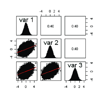
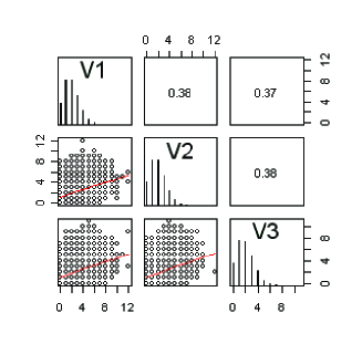
Figure 1: Comparing the simulated Normal (left) and Poisson (right) multivariate data with correlation matrix given in equation 11

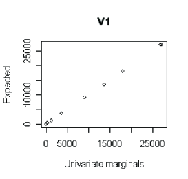
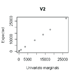
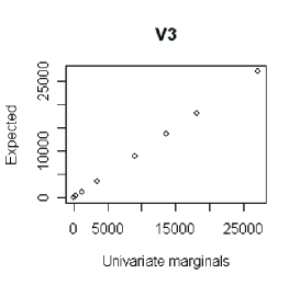
Figure 2: Comparing the marginal counts to Poisson expected values

4.2 Non-constant rate, non-constant correlations, and negative correlations

We next examine the case of a non-constant Poisson rate vector, unequal pairwise correlations, and negative correlations. All tests applied to the simulated data indicate that the pre-specified correlation matrix is maintained and that the marginal distributions are each Poisson. For sake of brevity we present only results for one configuration, but the same results were obtained for a wide range of vector rates and correlation matrices. In this test we set $\vec{\Lambda}=\{5,10,15\}$ and

(20)

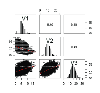
Figure 3: Test 2: Simulating multivariate Poisson data with correlation matrix given in equation 20

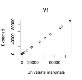
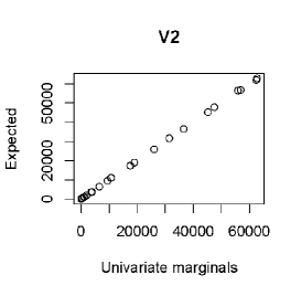
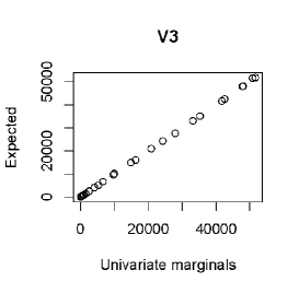
Figure 4: Comparing the Poisson marginals to the expected values

The simulated 3-variate Poisson data are shown in Figure 3 and the goodness of fit to a Poisson distribution is shown in the observed vs. expected scatter plots in Figure 4. We see that the estimated correlations are very close to those in the pre-specified $R$ (including the negative correlations) and that each of the marginal distributions closely fits a Poisson distribution.

4.3 Multivariate Poisson with Low Rates

Finally, we examine our approach for low rates ($\lambda\leq 4$). It is well known that the Poisson distribution with high rates ($\lambda>5$) is approximately a Normal distribution, and we thus expect the actual correlation of the multivariate Poisson random variables to match the desired correlation. However, as shown in Whitt (1976), the feasible correlation between two random Poisson variables is no longer in the range [$-1,1$], but rather [$min\_corr=corr(\Xi_{\lambda_{1}}^{-1}(U),\Xi_{\lambda_{2}}^{-1}(1-U)),max\_corr=corr(\Xi_{\lambda_{1}}^{-1}(U),\Xi_{\lambda_{2}}^{-1}(U))$]. In fact, Shin and Pasupathy (2007) show that when $\lambda_{1},\lambda_{2}\rightarrow 0$ the minimum feasible correlation $min\_corr\rightarrow 0$. Therefore, our transformation maps a correlation range of [$-1,1$] (multivariate normal) to a much smaller range [$min\_corr\geq-1,max\_corr\leq 1$]. Figure 5 illustrates the relationship between the desired correlation and the resulting actual correlation when generating bivariate Poisson data with low rates ($\lambda<1$).

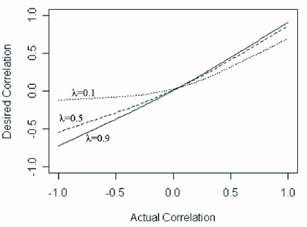
Figure 5: Comparing the desired correlation to the resulting actual correlation for low rates

We find that the relationship between the desired correlation and the actual correlation can be approximated by an exponential form:

$$R^{Pois}=a\times e^{bR^{N}}+c,$$

where the coefficient $a$, $b$ and $c$ can be estimated from the points ($\min\_corr$, -1), ($\max\_corr$, 1) and (0, 0):

$$a=-\frac{max\_corr\times min\_corr}{max\_corr+min\_corr}$$

$$b=log(\frac{max\_corr+a}{a})$$

$$c=-a$$

Figure 6 illustrates the simulation performance when using the above approximation to correct for the distortion in the resulting correlation. This is illustrated for the bivariate Poisson case with rates that range $(\lambda_{1},\lambda_{2})\in{(0.1,0.1),(0.1,0.5),(0.5,0.5),(0.5,0.9),(0.9,0.9)}$. The absolute difference between the actual and desired correlation is less then 0.05.

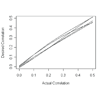
Figure 6: Comparing the desired correlation to the corrected actual correlation

5 Conclusions

Simulating multivariate Poisson data is essential in many real-world applications in a wide range of fields such as healthcare, marketing, management science, and many others. Current simulation methods suffer from computational limitations and restrictions on the correlation structure, and therefore are rarely used.

In this paper we propose an elegant way to generate multivariate Poisson data based on a multivariate Normal distribution with a pre-specified correlation matrix and Poisson rate vector. Because multivariate Normal and univariate Poisson simulators are implemented in many standard statistical software packages, implementing our method requires only a few lines of code.

We show that our method works well for different correlation structures (both negative and positive; and varying values) and for non-constant rates. We show that the method is highly accurate in terms of producing Poisson marginal distributions and the pre-specified correlation matrix.

APPENDIX: Generating Multivariate Poisson Data in R

    # Generate a p-dimensional Poisson
    # p         = the dimension of the distribution
    # samples   = the number of observations
    # R         = correlation matrix p X p
    # lambda    = rate vector p X 1
GenerateMultivariatePoisson<-function(p, samples, R, lambda){
        normal_mu=rep(0, p)
        normal = mvrnorm(samples, normal_mu, R)
        pois = normal
        p=pnorm(normal)
        for (s in 1:p){pois[,s]=qpois(p[,s], lambda[s])}
        return(pois)
}

    # Correct initial correlation between a
    # certain pair of series
    # lambda1   = rate of first series
    # lambda2   = rate of second series
    # r         = desired correlation
CorrectInitialCorrel<-function(lambda1, lambda2, r){
    samples=500
    u = runif(samples, 0, 1)
    lambda=c(lambda1,lambda2)
    maxcor=cor(qpois(u, lambda1), qpois(u, lambda2))
    mincor=cor(qpois(u, lambda1), qpois(1-u, lambda2))
    a=-maxcor*mincor/(maxcor+mincor)
    b=log((maxcor+a)/a, exp(1))
    c=-a
    corrected=log((r+a)/a, exp(1))/b
    corrected=ifelse ((corrected>1 | corrected<(-1)),
                       NA, corrected)
    return(corrected)
}

References

- Ahrens and Dieter (1982) Ahrens, J. H. and U. Dieter (1982). Computer generation of poisson deviates from modified normal distributions. ACM Transactions on Mathematical Software 8, 163 179.
- Devroye (1986) Devroye, L. (1986). Non-Uniform random variate generation, Chapter The Poisson Proess, pp. 245–250. Springer-Verlag.
- Hern dv lgyi (1998) Hern dv lgyi, I. T. (1998). Generating random vectors from the multivariate normal distribution. Working paper. Available at citeseer.ist.psu.edu/78434.html.
- Karlis (2003) Karlis, D. (2003). An em algorithm for multivariate poisson distribution and related models. Journal of Applied Statistics 30(1), 63–77.
- Krummenauer (1998) Krummenauer, F. (1998). Limit theorems for multivariate discrete distributions. Metrika 47(1), 47–69.
- Krummenauer (1999) Krummenauer, F. (1999). Efficient simulation of multivariate binomial and poisson distributions. Biometrical Journal 40(7), 823–832.
- Minhajuddin et al. (2004) Minhajuddin, A. T., I. R. Harris, and W. Schucany (2004). Simulating multivariate distributions with specific correlations. Journal of Statistical Computation & Simulation 74(81), 599–607.
- Ripley (1987) Ripley, B. D. (1987). Stochastic Simulation, Chapter Multivariate Distibutions, pp. 98–100. John Wiley & Sons.
- Shin and Pasupathy (2007) Shin k., and Pasupathy R. (2007). A Method For Fast Generation of Bivariate Poisson Random Vectors, Procceeding of the 2007 Winter Simulation Conference, pp. 472–479.
- Whitt (1976) Whitt, W.. (2007). Bivariate Distributions with Given Marginals, The Annals of Statistics 4(6), pp. 1280–1289.