Systematic Model Building Based on
Quark-Lepton Complementarity Assumptions

Abstract

In this talk, we present a procedure to systematically generate a large number of valid mass matrix textures from very generic assumptions. Compared to plain anarchy arguments, we postulate some structure for the theory, such as a possible connection between quarks and leptons, and a mechanism to generate flavor structure. We illustrate how this parameter space can be used to test the exclusion power of future experiments, and we point out that one can systematically generate embeddings in $Z_{N}$ product flavor symmetry groups.

In the literature, many approaches to a theory of lepton masses and mixings have been studied, such as descriptions by textures, GUTs, flavor symmetries, etc. (see LABEL:~Albright and Chen (2006) for a dedicated study). Most of these approaches are presented as possible, consistent theories predicting observables passing the current experimental constraints. However, it is difficult to obtain information on the parameter space as a whole which experiments are going to test, because it is not possible to compare individual models on a statistical basis. One possibility for such a test is generating a large sample of possibilities from very generic arguments. The most generic assumption, one can probably think of, are anarchic entries for the Yukawa couplings Hall et al. (2000). This procedure leads to very generic (and model-independent) distributions of the observables. However, one has to give up the belief in an underlying structure, such as a flavor symmetry. In this talk, we discuss a generic possibility to create a large parameter space of (valid) models using somewhat more structure. Our generic assumptions will be motivated by a possible connection between quarks and leptons, such as (see, e.g., Refs. Rodejohann (2004))

$$\theta_{12}+\theta_{C}\simeq\pi/4\simeq\theta_{23}\,.$$ (1)

This formula is often referred to as “quark-lepton complementarity” (QLC). In addition, we will illustrate how this approach can be systematically linked to flavor symmetries.

In our bottom-up approach Plentinger et al. (to appeara, to appearb); Winter (2007), we start with our generic assumptions in order to generate neutrino mass matrices including order one coefficients. We compute the neutrino oscillation observables from these matrices and check for compatibility with data. We call these matrices realizations. For all valid realizations, we then identify the leading order structure, which depends on the generic assumptions. We call these structures textures, since they contain the information on the origin of the Yukawa couplings. For example, for random mass matrices, one could identify texture zeros as the structure in the mass matrices. These textures can then be embedded in models in a specific framework. For example, one could use flavor symmetries to produce the structure in the textures. Note that there is a $1:n$ correspondence between realizations and textures, and there can be a $m:1$ correspondence between models and one specific texture. At the end, the interpretation of our results can be done in the reverse direction: From a model one obtains the texture, and for a (valid) texture, one immediately knows that there is a set of valid order one coefficients to reproduce this structure. There are several advantages of our approach. First, depending on the specific mechanism, one may not need diagonalization of the effective neutrino mass matrix, which simplifies the whole process tremendously. Second, from the generic assumptions, it is difficult to predict the outcome. Therefore, it is also difficult to introduce bias at this stage. Third, we will construct all possibilities given a set of generic assumptions, which will produce all new possibilities (textures, models) given our set of assumptions. And fourth, it is, of course, the objective of any systematic approach to study the parameter space. As a spin-off, one can easily demonstrate how experiments can test this parameter space most efficiently.

$M_{\nu}^{\rm Maj}=\left(\begin{array}[]{ccc}\epsilon^{2}&\epsilon^{2}&0\\ \epsilon^{2}&\epsilon&\epsilon^{2}\\ 0&\epsilon^{2}&1\end{array}\right)$

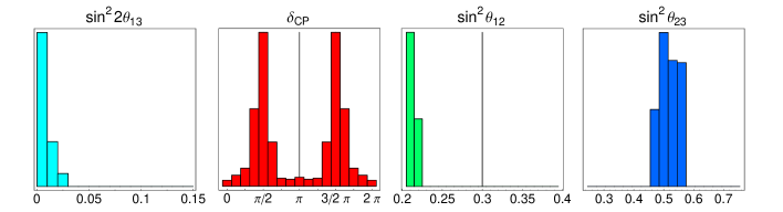
Figure 1: An example for a neutrino mass texture, and the corresponding distributions of the observables from the realizations leading to this texture. For details and more examples, see LABEL:~Winter (2007).

For the following, we will choose a specific generic assumption, which we have called “extended quark-lepton complementarity”. Based upon Eq. (1), we postulate that all masses and mixings in the quark and lepton sectors be described by powers of $\epsilon\simeq\theta_{C}$ as a potential remnant of a quark-lepton unified theory, i.e., by $\epsilon^{0}$, $\epsilon^{1}$, $\epsilon^{2}$, etc., where $\epsilon^{0}$ corresponds to maximal mixing for the mixing angles. One can easily demonstrate that all quark and lepton mass hierarchies can be described by powers of $\epsilon$, such as $\epsilon^{2}:\epsilon:1$ for a normal neutrino mass hierarchy, and all mixings as well Plentinger et al. (to appearb). For example, the Wolfenstein parameter $\lambda\simeq\epsilon$ allows for a parameterization of $V_{\mathrm{CKM}}$ (without phases), and the lepton mixing might be described by $U_{\mathrm{PMNS}}=V_{\mathrm{CKM}}^{\dagger}V_{\mathrm{Bimax}}$ as a product of $V_{\mathrm{CKM}}$ and a mixing matrix with two maximal mixing angles as a special case Jezabek and Sumino (1999). Using our generic assumptions, we generate all possible realizations, filter the realizations compatible with data, and calculate the textures by identifying the leading order in $\epsilon$. Note that, compared to the texture zero case, we allow for more structure in the textures: The entries can be $1$, $\epsilon$, $\epsilon^{2}$, or $0$, where $0$ corresponds to $\mathcal{O}(\epsilon^{3})$. Of course, keeping this type of information in the textures is only relevant as long as one wants to go one step further: We will illustrate how the powers of $\epsilon$ can be connected to specific models, such as discrete flavor symmetries.

Let us now introduce our procedure for the (effective) $3\times 3$ case. First, we generate all possible pairs $\{U_{\ell}$, $U_{\nu}\}$ using the standard parameterization for the unitary mixing matrices. We generate all possible mixing angles $\sin\theta_{ij}^{\alpha}\in\{1/\sqrt{2},\epsilon,\epsilon^{2},0\}$, and all possible real phases ($0$ or $\pi$). Then we calculate $U_{\rm PMNS}$ by

$$U_{\rm PMNS}=U_{\ell}^{\dagger}U_{\nu}\,,$$ (2)

read off the mixing angles and observable phases, and select those realizations with mixing angles being compatible with current data at the $3\sigma$ confidence level (cf., LABEL:~Plentinger et al. (to appeara)). For each valid realization, we then find, for instance, the corresponding Majorana mass matrix texture by computing

$$M_{\nu}^{\rm Maj}=U_{\nu}M_{\nu}^{\rm diag}U_{\nu}^{T}\,,$$ (3)

expanding in $\epsilon$, and by identifying the first non-vanishing coefficient. Here the assumptions for $M_{\nu}^{\rm diag}$ are taken from extended QLC as well, such as $m_{1}:m_{2}:m_{3}=\epsilon^{2}:\epsilon:1$ for the normal mass hierarchy. In this procedure, diagonalization is not necessary compared to generating the entries in $M_{\nu}^{\rm Maj}$ directly.

As a result, a systematically generated set of textures and sum rules is obtained Plentinger et al. (to appeara). For example, one obtains a “diamond-shaped” texture which can be produced by the two maximal mixing angles in the lepton sector ($\theta_{12}^{\ell}$ and $\theta_{23}^{\ell}$) and one maximal mixing angle in the neutrino sector ($\theta_{13}^{\nu}$). In addition, one can study the distributions of observables obtained from the set of realizations. For example, a large mixing $\sin^{2}2\theta_{13}$ close to the current bound is indeed preferred from the complete set of valid realizations. Furthermore, since $\theta_{12}$ can only be obtained by the matrix multiplication in Eq. (2) from maximal and Cabibbo-like mixing angles, future precision measurements of $\theta_{12}$ will exert pressure on the parameter space.

As the next step, one can introduce complex phases in the effective $3\times 3$ mechanism by systematically generating all possible phases with uniform distributions Winter (2007). If one then studies the distributions of observables as a function of the texture, one finds that these distributions are very texture dependent. For example, Figure 1 shows a texture preferring small $\sin^{2}2\theta_{13}$, maximal CP violation, $\theta_{23}$ close to the best-fit value, and $\theta_{12}$ close to the currently allowed lower bound. For the present example, a detection of large $\sin^{2}2\theta_{13}$, or a confirmation of $\theta_{12}$ close to the current best-fit value would clearly disfavor the texture. It turns out that there are many such qualitatively different cases as a function of the texture one uses. In addition, one finds peaks close to CP conservation in some of the $\delta_{\mathrm{CP}}$ distributions, where the deviations from $0$ or $\pi$ are of the order $\theta_{C}$. Such peaks may motivate a $\delta_{\mathrm{CP}}$ precision of future high precision measurements at the level of $\theta_{C}\simeq 11^{\circ}$, as it could be obtained at a neutrino factory ($1\sigma$) Huber et al. (2005).

$M_{\ell}$	$M_{D}$	$M_{R}$
$\left(\begin{array}[]{ccc}0&\epsilon^{2}&1\\ 0&\epsilon^{2}&\epsilon\\ 0&\epsilon^{2}&1\\ \end{array}\right)$	$\left(\begin{array}[]{ccc}\epsilon&0&0\\ \epsilon&1&\epsilon\\ \epsilon&1&0\\ \end{array}\right)$	$\left(\begin{array}[]{ccc}\epsilon&\epsilon&0\\ \epsilon&1&0\\ 0&0&1\\ \end{array}\right)$
$\displaystyle(\nu_{1}^{c},\nu_{2}^{c},\nu_{3}^{c})$ $\displaystyle=$ $\displaystyle(1,0,1)\quad(0,3,2)\quad(3,3,0)$ $\displaystyle(\ell_{1},\ell_{1},\ell_{3})$ $\displaystyle=$ $\displaystyle(4,3,2)\quad(0,1,0)\quad(0,2,2)$ $\displaystyle(e_{1}^{c},e_{2}^{c},e_{3}^{c})$ $\displaystyle=$ $\displaystyle(3,0,2)\quad(2,0,2)\quad(1,2,0)$

Table 1: First row: A possible texture obtained in the seesaw case (for small $\sin^{2}2\theta_{13}$ and a normal hierarchy) Plentinger et al. (to appearb). Second row: A set of possible quantum numbers for a $Z_{5}\times Z_{4}\times Z_{3}$ flavor symmetry. Note that common pre-factors can be absorbed in the absolute mass scale, and that a texture zero corresponds to $\mathcal{O}(\epsilon^{3})$.

Our procedure can be extended to the seesaw mechanism by parameterizing the $6\times 6$ neutrino mass matrix in terms of three unitary matrices and the corresponding mass eigenvalues in a similar way Plentinger et al. (to appearb). Similar to the $3\times 3$ case, the charged lepton sector is not assumed to be diagonal. We find $1\,981$ different textures generated with the assumption of $\sin^{2}2\theta_{13}$ small and of a normal neutrino mass hierarchy. One example, which can be realized with $(\theta_{12},\theta_{13},\theta_{23})=(33^{\circ},0.2^{\circ},52^{\circ})$, is shown in Table 1 (upper row). Special cases, such as $M_{D}$ symmetric, are rare in our sample. However, about a quarter of all realizations lead to $M_{R}$ being almost diagonal. For the mass hierarchies, we obtain many cases with mild hierarchies in $M_{D}$ and $M_{R}$. Not surprisingly, charged lepton mixing is quite substantial in many cases. In fact, for about one third of all possible realizations, there are three maximal mixing angles in $U_{\ell}$.

Let us now discuss what the Yukawa coupling structure, such as the one shown in Table 1, is actually good for. For example, masses for quarks and leptons may arise from higher-dimension terms via the Froggatt-Nielsen mechanism Froggatt and Nielsen (1979) in combination with a flavor symmetry:

$$\mathcal{L}_{\mathrm{eff}}\sim\langle H\rangle\,\epsilon^{n}\,\bar{\Psi}_{L}\Psi_{R}\,.$$ (4)

In this case, $\epsilon$ becomes meaningful in terms of a small parameter $\epsilon=V/M_{F}$ which controls the flavor symmetry breaking. The integer power of $\epsilon$ is solely determined by the quantum numbers of the fermions under the flavor symmetry (see, e.g., Refs. Plentinger et al. (to appearb); Enkhbat and Seidl (2005)). Using discrete Abelian $Z_{N}$ product flavor symmetry groups, one can now try to reproduce our textures by calculating the specific embeddings Plentinger et al. (in preparation). For instance, one can discuss how much complexity is actually needed to reproduce almost all of our $1\,981$ textures. While one can find embeddings for simple textures already for symmetries such as $Z_{4}$, it turns out, that one can find model embeddings for about $60\%$ of our textures for $Z_{5}\times Z_{4}\times Z_{3}\times Z_{2}$. Therefore, with that amount of complexity, one can almost reproduce any viable texture. As one non-trivial example, consider the $Z_{5}\times Z_{4}\times Z_{3}$ discrete symmetry embedding for the texture in Table 1 (upper row): One possible set of quantum numbers is given in Table 1, lower row.

In summary, we have demonstrated how our automatic procedure can be used to automatically generate valid textures, corresponding order one coefficients compatible with data, and specific models including the charge assignments at the example of a discrete $Z_{N}$ product flavor symmetry groups. While the generation is bottom-up, the interpretation of our results can be performed in a top-down fashion: A model predicts a form of the mass matrix (texture), and this form is known to fit data with proper order one coefficients (realization). As potential applications, our approach can be used of parameter space studies for the observables or for theories (models), as well as for finding new models. As a spin-off, the exclusion power of experiments in the generated parameter space can easily be tested.

Acknowledgments I would like to acknowledge support from the Emmy Noether program of Deutsche Forschungsgemeinschaft.