Thermodynamics from a scaling Hamiltonian

Abstract

There are problems with defining the thermodynamic limit of systems with long-range interactions; as a result, the thermodynamic behavior of these types of systems is anomalous. In the present work, we review some concepts from both extensive and nonextensive thermodynamic perspectives. We use a model, whose Hamiltonian takes into account spins ferromagnetically coupled in a chain via a power law that decays at large interparticle distance $r$ as $1/r^{\alpha}$ for $\alpha\geq 0$. Here, we review old nonextensive scaling. In addition, we propose a new Hamiltonian scaled by $2\frac{(N/2)^{1-\alpha}-1}{1-\alpha}$ that explicitly includes symmetry of the lattice and dependence on the size, $N$, of the system. The new approach enabled us to improve upon previous results. A numerical test is conducted through Monte Carlo simulations. In the model, periodic boundary conditions are adopted to eliminate surface effects.

I Introduction

A good description of magnetic ordering phases illuminates concepts about the critical behavior and possible applications of magnetic devices. We know that the magnetic behavior of systems decreases when the dimensionality of a physical system decreases. This led to incorrect beliefs that prompted specialists to lose interest in one-dimensional systems. However, several theoretical and practical aspects, which appeared in the physical properties of one-dimensional systems, caused specialists to reverse those beliefs.pre70 ; mplb17 ; pra45 ; prl76 ; prl86 ; prb56 ; prb34 ; PGaNat416 ; Zedler ; Curilef ; prbCannas

Recently, ferromagnetism in one dimension has been reported in various systems. Transitions between two different magnetic ordering phases are obtained using different approaches and considerations, and we will discuss some of these. First, microscopic anomalies lead to important modifications in the thermodynamic properties of systems. As a consequence, it is suggested that anisotropy barriers contribute to the novel effect.PGaNat416 Second, the Gibbs potential of a one-dimensional metal at constant magnetization is calculated to second order in the screened electron-electron interaction. At zero temperature, a possible paramagnetic-ferromagnetic quantum phase transition was found in one-dimensional metals, which must be first order.Zedler Finally, a special Hamiltonian considers long-range interactions through a power law that decays at large interparticle distances. It has been shown that if the range of interactions decreases, the critical temperature trend disappears, but if the range of interactions increases, the trend of the critical temperature approaches the mean field approximation. The crossover between these two limiting situations is preliminarily discussed.Curilef . That crossover is a consequence of long-range interactions, and we use it to illustrate the nonextensive perspective of the thermodynamics.

To describe the behavior of systems with long range interactions, some scalings approaches kac have been introduced in the literature. In the present work, we carefully discuss the thermodynamic behavior of systems with microscopic long-range interactions, taking into account a method of implementing periodic boundary conditions (section III) via a scaling Hamiltonian (section IV). Previously, the critical temperature between two states of different magnetic ordering was obtained in a spin-$\frac{1}{2}$ Ising linear chain, where the range of interactions is, at least, comparable to the size of the chain. However, in order to obtain suitable thermodynamic behavior, in accordance with impositions from extensivity, we improve the so called nonextensive scaling (section IV) for a symmetric one-dimensional lattice.

This paper is organized as follows: In section II, we introduce the nonextensive perspective of thermodynamics. In section III, we explain the method of implementing periodic boundary conditions to eliminate surface effects. In section IV, we review the Tsallis scaling to get a formalism of the thermodynamics from a scaling Hamiltonian and then explain some important results about the presented formalism. In section V we summarize our work and make some concluding remarks.

II Nonextensive Thermodynamics

In this section, we introduce some fundamental facts about the nonextensive perspective of thermodynamics, which can be easily illustrated by long-range interaction systems.

II.1 Tsallis Scaling:

This method is useful for scaling thermodynamic quantities that depend strongly on the size of the system with long-range microscopic interactions. The explicit form of Tsallis scaling appears by evaluating the internal energy per particle. We take into account interparticle potentials $v(r)$ with an attractive tail that decays as:

$$v(r)=\frac{1}{r^{\alpha}}.$$ (1)

The original Tsallis scaling, from the asymptotic trend of $U_{N}$, for systems in one dimension, is given by:

$$N^{*}=\left\{\begin{array}[]{llll}&(N^{1-\alpha})/{(1-\alpha)}&\text{for }&0\leq\alpha<1\\ &\log(N)&\text{for }&\alpha=1\\ &1/{(\alpha-1)}&\mbox{for }&\alpha>1.\end{array}\right.$$ (2)

The present scaling has been revised by several authors and applied to different physical situations. The scaling was expressed in a most appropriate form for discrete systemsprbCannas and was previously written as $2^{\alpha}N^{*}$. Indeed, in the present work we reviewed this kind of scaling and included it as a best approach.

II.2 Mean Field Approximation

We consider a one dimensional model of $N$ spins-$\frac{1}{2}$. If the coupling is long-range, surface effects appear and become important. This fact requires working with very large systems. However, surface effects can be ignored, even in moderately sized systems, by applying periodic boundary conditions. This is a nontrivial task when long range interactions are considered. However, it is possible to do in a suitable form, which is introduced in section III. The model is described by the Hamiltonian:

$$H=-\sum_{i,j=1}^{n}J(i-j)s_{i}s_{j},$$ (3)

where $n$ is the number of particles in every cell, and $s_{i}=\pm 1\;\;\;\forall i$. The difference $(i-j)$ represents the distance between two sites. A non external magnetic field is considered. The coupling decays as a power law given by:

$$J(i-j)=\frac{J}{|i-j|^{\alpha}},$$ (4)

where $J$ is a positive parameter which measures the strength of the coupling. In previous works, these kinds of systems have been discussed by several authors.pre70 ; mplb17 ; pra45 ; prl76 ; prl86 ; prb56 ; prb34 ; Curilef ; prbCannas ; Tsallis A common behavior has been conjectured Tsallis for generic systems with arbitrary (long or short)-range interactions. With the aim of calculating the mean value of the Hamiltonian, we proceed in the same way as in the Eq.(12). $\langle H\rangle=\sum_{i=1}^{N}E(N)s_{i}$, where $E(N)=\frac{1}{2}J{N}^{*}\langle s\rangle$; the factor $\frac{1}{2}$ ensures that we do not count the same pair of spin twice and in this view; ${N}^{*}$ (defined in the Eq.(12)) represents the effective number of the nearest neighbor spins. The quantity $\langle s\rangle$ is the average spin per site. This assumption helps us recover all the results for systems with long-range microscopic interactions in a similar manner to the traditional mean field approximation. This treatment can be extended even if the external magnetic field is nonzero.

So, the average spin per site of the lattice is given by $\langle s\rangle=\tanh\left[\frac{1}{2}\beta{N}^{*}J\langle s\rangle\right].$ In the absence of an external magnetic field, the magnetization is zero for a high temperature paramagnetic phase, and it will be nonzero at lower temperatures where the spins have spontaneously aligned. For the present system, the internal energy is given by $U(N)=\frac{1}{2}N{N}^{*}J\langle s\rangle^{2}.$ Hence, the internal energy is given by $U(N)=NN^{*}U_{1}$. The extensive property imposes observables to be a linear homogeneous function of $N$ and $U(\lambda N)=\lambda U(N)$. However, when long range interactions are included, this property is violated, and it is easy to show that thermodynamic functions are homogeneous of degree $1+|\alpha-1|$ for $\alpha<1$ (and logarithmic of $N$ for $\alpha=1$).

In addition, we expect that the internal energy of a magnetic system with long-range interactions adopts the following form: $U(S,M,N)=N{N}^{*}U_{1}(S/N,M/N),$ where $U_{1}$ is a function per particle of the entropy, $S$, and magnetization, $M$. Generally, we could write other extensive variables like $X=V,A,L,P,\cdot\cdot\cdot$ (representing the volume, area, length, and polarization, respectively) as follows:

$$U(\lambda S,\lambda X,\lambda N)=\lambda^{1+|\alpha-1|}U(S,X,N).$$ (5)

Hence, a problem with defining the thermodynamic limit persists for $\alpha\leq 1$, in accordance with Eq.(5). The linearity is only recovered for $\alpha>1$. As previously observed, a strong dependence on the size of the system obstructs the behavior of the thermodynamic functions and relations.

II.3 Tsallis Conjecture:

As a possible way to solve this problem, Tsallis conjectured that quantities like energy (like internal energy, Helmholtz and Gibbs energies, and thermodynamic potentials per particles) and intensive variables (like $T$ as in temperature, $H$ as in magnetic field) scale with $N^{*}$. Consistency of this conjecture is shown as follows

$$\frac{G_{N}}{N^{*}N}=\frac{U_{N}}{N^{*}N}-\frac{T}{N^{*}}\frac{S_{N}}{N}-\frac{H}{N^{*}}\frac{M}{N}$$ (6)

in the thermodynamic limit. Observables per particle and intensive variables are divergent when interactions are long-range. However, scaling quantities are convergent anywhere. This kind of scaling presents a standard thermodynamic structure because it preserves the Euler and Gibbs-Duhem relationsAbe . By the same reasoning, it is possible to define scaling quantities as follows: $G_{N}^{*}=G_{N}/N^{*}$, $U_{N}^{*}=U_{N}/N^{*}$, $T^{*}=T/N^{*}$ and $H^{*}=H/N^{*}$. With these definitions the previous equation is given by

$$\frac{G_{N}^{*}}{N}=\frac{U_{N}^{*}}{N}-T^{*}\frac{S_{N}}{N}-H^{*}\frac{M}{N}.$$ (7)

At this stage, we focus on some problems related to the interpretation of the Eq.(7). For instance, the measured temperature is not $T^{*}$, it is $T$; the measured internal energy per particle is not $U_{N}^{*}$, it is $U_{N}$, etc.

III Periodic Boundary Conditions

If the range of microscopic interactions is smaller than the size of the system, thermodynamic properties are obtained from standard calculations. However, if interactions are long-range, surface effects appear and begin to be important for all finite sizes of systems. The calculation of thermodynamic quantities must be carefully done. Long-range interactions are often defined as those that do not fall faster than $1/r^{D}$, where $D$ is the space dimension of the system. A first approach requires increasing tremendously the size of the box. In general, periodic boundary conditions are applied in order to eliminate surface effects in the calculation of the thermodynamics properties of systems. This can be exemplified by a central cell, which is repeated throughout space to construct an infinite lattice. During the course of the present study, if a particle moves in the central cell, its periodic images move with the same orientation in everyone of the other cells. Thus, as a particle leaves the central cell, one of its images will enter through the opposite face. There are no walls at the boundary of the central cell, and the system has no surface. In general, particles interact with a potential of the following form $v(z)=\lim_{L\rightarrow\infty}\sum_{k=-L}^{L}g(|k+z|)$, where the summation over $k$ represents all contributions over replicated images. Thus, summations can be written in the following manner:

$$\sum_{k=-L}^{L}g(|k+z|)=\sum_{k=1}^{L}g(k-z)+g(|z|)+\sum_{k=1}^{L}g(k+z).$$ (8)

Two particular cases (the $1/z$ and the logarithmic potential) have been discussed in a previous workPhysA340 .

Certainly, forces are obtained from $f(z)=-dv(z)/dz$. Due to the symmetry of the lattice, it is easy to show that contributions to the net force on every particle from all their images vanish. Thus, periodic summations of forces do not practically depend on the nature of interactions. In this manner, the net force ($f_{N}=-dg(z)/dz-F_{L}$) converges as quickly as the sum $F_{L}$ converges

$$F_{L}\sim\sum_{k=1}^{L}\left[\frac{dg(k+z)}{dz}+\frac{dg(k-z)}{dz}\right],$$ (9)

where $-1/2<z<1/2$ and $k\gg 1$. $dg(z)/dz$ represents the force of a couple of particles in the central cell, and $F_{L}$ contributions of all replicated cells in all space. If we take into account a potential like Eq.(1), net force converges in the same manner as summations from Eq.(9):

$$F_{L}\sim -\sum_{k=1}^{L}\left[\frac{1}{(k+z)^{\alpha+1}}-\frac{1}{(k-z)^{\alpha+1}}\right]$$

$$\approx 2z(1+\alpha)\sum_{k=1}^{L}\frac{1}{k^{2+\alpha}}$$

$$\propto 4z\left(1-L^{-1-\alpha}\right).$$

If $L\geq 1$, contributions of particles and their images are included.

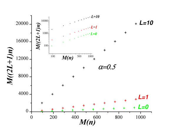
Figure 1: Linearity of magnetization is shown for $L=0,\,1$ and $10$ and several values of $n$ with $N=(2L+1)n$. We plot $M(\lambda n)$ versus $M(n)$, where $\lambda=(2L+1)$. We see that the slope is $\lambda$. In the inset we plot the same in log-log scale. The slope is 1. This fact emphasizes that magnetization is a linear homogeneous function of the size of the system.

IV Scaling Hamiltonian and Numerical Test

We consider a symmetric chain of $n$ spin-$\frac{1}{2}$ in a central cell that it is replicated $L$ times over both sides. So, the total number of particles $N=(2L+1)n$. Thus, we study the system via the Hamiltonian of the Eq.(3)and apply periodic boundary conditions in the manner introduced in section III. We write the coupling as follows

$$J(K)=\frac{1}{2}\sum_{l=-L}^{l=L}\frac{J_{\alpha}^{L}(n)}{|nl+K|^{\alpha}}.$$ (11)

Hence, in order to obtain the scaling, we can determine it using the tendency of internal energy, similar to Tsallis Tsallis . Taking into account the symmetry of the chain and the continuous limit, we derive the following integral:

$$U_{N} \propto 2\int_{1}^{N/2}drg(r)v(r)$$ (12)

$$\propto 2\frac{(N/2)^{1-\alpha}-1}{1-\alpha},$$

where $g(r)$ (the pair distribution function) approaches 1 for $r\gg 1$. Indeed, from Eq.(12) the scaling coupling can be written in the approach:

$$J_{\alpha}^{L}(n)=\left\{\begin{array}[]{lll}J/2^{\alpha}{N^{1-\alpha}}&\text{if $\alpha<1$}\\ J/2\ln N&\text{if $\alpha=1$ }\\ ({1-\alpha})J/{2}&\text{if $\alpha>1$ }\end{array}\right.$$ (13)

where $J_{\alpha}^{L}(n)$ measures the strength of the coupling that depends on the size $n$ of the system. If we combine Eq.(11) and (13) and substitute the result into Eq.(3), then we obtain the scaling Hamiltonian that we used to carry out numerical results with the Monte Carlo procedure. At this stage, we emphasize that the scaling, in terms of $N^{*}$, is $2^{\alpha}{N^{*}}$ for $\alpha<1$ and $2{N^{*}}$ for $\alpha\geq 1$. It has been well expressed in Eq.(13) for symmetric lattices. Previously, (see for instance Ref.prbCannas ) the scaling coupling was defined in the old form $({1-\alpha})J/{2^{\alpha}}$ and not as the new form $({1-\alpha})J/{2}$ (from Eq.(13)) for $\alpha\geq 1$, for a discrete lattice. Hence, if the old scaling is applied to systems whose most important geometrical property is symmetry, then it would poorly represent the trends in thermodynamic quantities.

Thermodynamics describes the behavior of systems with many degrees of freedom after they have reached a state of thermal equilibrium. Furthermore, their thermodynamic state can be specified in terms of a few parameters called state variables. At equilibrium, this method of scaling the Hamiltonian allows observables to be linear with the number of particles.

IV.1 Linearity of extensive quantities

It is well known that thermodynamic quantities have to behave linearly relative to $N$, the size of the system. For the present specific model of a chain of spins with ferromagnetic long-range interactions, due to the form of the scaling Hamiltonian, we expect that the linearity of internal energy was completely satisfied and $U(\lambda{n})={\lambda}U(n)$. This goes against the nonextensive view of the thermodynamics, which predicts a nonlinear homogeneous behavior of internal energy, like Eq.(5). In addition, according to the Tsallis conjecture, we expect that other extensive quantities also become linear with $N$. In Fig. 1, the linearity of magnetization was tested from simulations for $L=0,\,1$ and $10$ and several values of $n$, where $N=(2L+1)n$. We depict several values of magnetization $M(\lambda{n})$ versus $M(n)$, where $\lambda=(2L+1)$. A simple inspection reveals linearity, i.e.$M(\lambda{n})={\lambda}M(n)$. Simulation points depict right lines that differ only in their slopes. This fact is highlighted in the inset of Fig. 1 in log-log scale, where we observe that all lines are parallel, whose slope is 1, an indicator of linearity. So, we see that the linearity of an observable is satisfied when it is different from the internal energy, similar to the case of magnetization.

IV.2 Improvement of the critical temperature

Phase transition characterization is obtained in several ways. One of the most adequate approaches is to define the critical point for finite systems by the Binder method. To do so, we need to assess the Binder cumulants of fourth order, which are defined as $u_{n}=1-\langle{s}^{4}\rangle/3\langle{s}^{2}\rangle^{2}$. Cumulants $u_{n}$ as a function of the temperature, intersect at a common point for several sizes, $n$, of the system. This point is the critical temperature that depends on the range of interactions $\alpha$. We test the trend of the critical temperature and plot it as a function of $\alpha$ using the scaling Hamiltonian, and we compare the present result to the trend obtained previously from the old scaling. In the present study, we carry out on a linear chain, where the number of particles in the central cell is $10^{2}\leq n\leq 10^{3}$. On the one hand, the effective number of particles of the samples $N=(2L+1)n$ depends on the number, $L$, of replicas. On the other hand, the computation time depends just on $n$, not on $L$. We see that $L=10^{3}$ is good enough, to compute in the thermodynamic limit and, eliminate unnecessary sources of numerical fluctuations. For $0\leq\alpha\leq 1$, the critical temperature approaches the mean field value (e.g., for $\alpha=0.5$, $T_{c}/T_{c}^{MF}=0.985\pm 0.005$). But when $\alpha>1$, results from different scalings do not coincide and they are different from the values predicted by the mean field approximation. In Fig. 2, the trend of the critical temperature is depicted as a function of $\alpha$. We include results in the range $0\leq\alpha\leq 2$ for the critical temperature scaled in the manner presented.

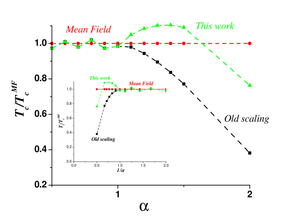
Figure 2: The trend of the critical temperature as a function of $\alpha$, the range of interaction. For $0\leq\alpha\leq 1$, the critical temperature coincides with the mean field value. The new trend is compared to the old one. In the inset we show the critical temperature as a function of $1/\alpha$

V Summary and Concluding Remarks

In the mean field approximation, the state of magnetic ordering of a chain of spins with microscopic long-range interactions constitutes an example of ferromagnetism in one dimension. Because interactions are short range (e.g., first neighbors) in the standard Ising model, no magnetic ordering is observed in one dimension. These approaches define two limiting cases. In the present work, the main goal is to describe the crossover between these two limiting cases in a suitable manner. First, if we take a scaling Hamiltonian, the nice extensive property is recovered, and the thermodynamic quantities are linear homogeneous functions against the homogeneous function of degree $1+|\alpha+1|$, which are obtained if the Hamiltonian is not scaled. Second, an improvement to the nonextensive scaling is proposed here to obtain a more suitable method of describing the thermodynamic behavior trend in this kind of systems for $\alpha>1$. In the $N\rightarrow\infty$ limit, we compare old scaling: $2^{\alpha}N^{*}$, versus new scaling: $2N^{*}$. Third, periodic boundary conditions can be used in the approach, using infinite replications of a central cell and considering the contribution over all space. It has been shown that forces converge rapidly. However, potentials increase with the size of the system. The thermodynamic limit was reached in a numerical approach, with a few particles in the central cell and a finite number, $L$, of replications. Finally, we focus our attention on the Tsallis scaling (not the Tsallis conjecture); which is sufficient to solve the problem of the loss of linearity for thermodynamic quantities like energy and intensive variables, if we use it conveniently in the Hamiltonian.

References

- (1) H. Chamati, D. Dantchev, Phys. Rev. E 70, 066106 (2004).
- (2) H. Chamati, N. Stonchev, Mod. Phys. Lett. 17, 1187 (2003); J. Phys. A: Math. Gen 33, L187 (2000).
- (3) R. Minieri, Phys. Rev. A 45 3580 (1992).
- (4) E. Luijten and H. W. J. Blöte, Phys. Rev. Lett. 76, 1557 (1996).
- (5) E. Luijten and H. Meingfeld, Phys. Rev. Lett. 86, 5305 (1996).
- (6) E. Luijten and H. W. J. Blöte, Phys. Rev. B 56, 8945 (1997).
- (7) J. O. Vigfusson, Phys. Rev. B 34 3466 (1986).
- (8) P. Gambardella, A. Dallmeyer, K. Maiti, M.C. Malagoli, W. Eberhardt, K. Kern, and C. Carbone, Nature 416, 301 (2002).
- (9) P. Zedler and P. Kopietz, Phys. Rev. B 72, 184404 (2005)
- (10) S. Curilef, L. A. del Pino and P. Orellana, Phys. Rev. B 72, 224410 (2005)
- (11) S. Cannas, F. Tamarit, Phys. Rev. B 54, 12661 (1996).
- (12) M. Kac, G. Uhlenbeck, P. C. Hemmer, J. Math. Phys. 4, 216 (1963)
- (13) C. Tsallis, Fractals 3, 541 (1995).
- (14) S. Abe and A. K. Rajagopal, Phys. Lett. A 337, 292 (2005)
- (15) S. Curilef, Physica A 344, 456 (2004)