A method of open cluster membership determination

Abstract

A new method for the determination of open cluster membership based on a cumulative effect is proposed. In the field of a plate the relative $x$ and $y$ coordinate positions of each star with respect to all the other stars are added. The procedure is carried out for two epochs $t_{1}$ and $t_{2}$ separately, then one sum is subtracted from another. For a field star the differences in its relative coordinate positions of two epochs will be accumulated. For a cluster star, on the contrary, the changes in relative positions of cluster members at $t_{1}$ and $t_{2}$ will be very small. On the histogram of sums the cluster stars will gather to the left of the diagram, while the field stars will form a tail to the right. The procedure allows us to efficiently discriminate one group from another. The greater the distance between $t_{1}$ and $t_{2}$ and the more cluster stars present, the greater is the effect. The accumulation method does not require reference stars, determination of centroids and modelling the distribution of field stars, necessary in traditional methods. By the proposed method 240 open clusters have been processed, including stars up to $m<13$. The membership probabilities have been calculated and compared to those obtained by the most commonly used Vasilevskis-Sanders method. The similarity of the results acquired the two different approaches is satisfactory for the majority of clusters.

1 Introduction

Various methods based on the analysis of positions, proper motions, radial velocities, magnitudes and their combinations have been proposed to determine the members of open clusters.

The first mathematically rigorous procedure for determination of open cluster membership was developed by Sanders (Sanders (1971)) with a statistical analysis of proper motions. It is also the most widely used method. Sanders’s approach is based on the model of overlapping distributions of field and cluster stars in the neighborhood and within the region of visible grouping of stars, introduced by Vasilevskis et al. (Vasilevskis (1958)).

Vasilevskis’s model implies that proper motion dispersion of cluster members is caused by observational and measurement errors assumed to be normally distributed. Thus the distribution of cluster stars is represented by a bivariate normal frequency function. The dispersion of field stars is due to not only the errors referred to above, but also to peculiar motion and differential galactic rotation. Therefore the field star distribution is not expected to be random, but rather to have a preferential direction and not normal distribution. However, in a first approximation a bivariate normal ellipsoidal distribution function was assumed for field stars, the major axis of the ellipse being parallel to the galactic plane.

Thus, Sanders’s equations contain 8 unknown parameters to be determined: the number of cluster members, x and y components of two centroids, one circular and two elliptical dispersions. This system is solved by a maximum likelihood method (Sanders Sanders (1971)). The probability of stars being cluster members is calculated by frequency functions with determined parameters.

Slovak (Slovak (1977)) tested the Vasilevskis-Sanders method by modelling the proper motion distribution in the surroundings of a cluster. He proved the uniqueness and convergence of solutions of the system, provided that errors are represented by a Gaussian distribution and open clusters have no significant internal motion. But if there is noticeable motion within a cluster or it rotates then the above method fails.

Cabrera-Caño and Alfaro (Cabrera-Cano Alfaro1 (1985)) improved the numerical techniques for obtaining the above parameters. McNamara and Schneeberger (McNamara Schneeberger (1978)) showed that the final probabilities could be influenced by various weight groups. Zhao and He (Zhao He (1990)) provided a method for treating data with different accuracies.

However all these improvements did not treat the problem of star distribution model on which the membership probabilities are based. Even if the hypothesis of a normal distribution of field stars is realistic for some clusters, the centroids of field and cluster stars sometimes are too close to be well discriminated. The parametric model also fails when the cluster member-to-field star ratio is small. The Vasilevskis-Sanders method does not work in the case of significant internal motion in a cluster or its rotation.

To overcome some of the problems arising from the parametric Vasilevskis-Sanders method, especially the star distribution modelling, Cabrera-Caño and Alfaro (Cabrera-Cano Alfaro2 (1990)) developed a more general, non-parametric method of membership determination. Here no assumptions were made about the nature of cluster and field star distributions and allowed for the use of photometric data. Each cluster needed careful individual study.

So, the actual distribution of cluster and field stars, especially the latter, may not be fitted by a Vaselevskis-Sanders model; the centroids for the two groups may be too close to be distinguished; the reliability of the method depends on the cluster-to-field star ratio; in the case of significant internal motions or rotation of a cluster the traditional method fails.

In the next section we introduce a new method for the discrimination of cluster stars from surrounding field stars based on a cumulative effect using positions and proper motions. We do not try to overcome all the difficulties of traditional methods, though we offer another approach that enlarges the statistical distance between the two populations - cluster members and field stars - by revealing the group of stars with the least relative velocities. The advantage of this method is that no assumption is made about the distribution of field stars and determination of centroids is avoided. However, in order to determine probabilities we still have to assume a normal bivariate distribution for clusters. Another advantage of the method is that reference stars are not necessary: the discrimination of cluster members is most effective by rectangular coordinates. These features of the method allow us to increase the statistical distance between the two populations. The most noticeable advantage of the accumulation method is its ability to reveal dynamic structures within the clusters if there are any.

2 The method

We consider a cluster as a gravitationally bound system with a bulk motion relative to surrounding galactic field stars. Field stars are characterized by more or less random velocities. Therefore the cluster members must show regular motion, while the field stars move realtively irregularly.

We consider rectangular coordinates of stars in the field of a plate (or CCD array), measured in two epochs $t_{1}$ and $t_{2}$. The relative $x$ and $y$ positions of each star with respect to all the other stars in the area are added. If the two epochs are well separated, then for a field star the differences of the relative coordinate positions in the two epochs will be accumulated. For cluster stars, the changes of relative positions of physical members at $t_{1}$ and $t_{2}$ must be very small and their sum will be minimal. The more cluster stars, the bigger is the effect. If one draws a histogram of differences, the stars with minimal relative velocities (which we consider more likely to be cluster members) will gather to the left of the diagram, while the field stars will form a tail to the right. Thus, the procedure allows us to efficiently discriminate one group from another, avoiding the use of reference stars.

For each star the following quantities are calculated:

$$S_{x_{i}}^{\prime}=\sum_{j=1}^{N}|{x_{i}^{\prime}-x_{j}^{\prime}}|,\\ S_{y_{i}}^{\prime}=\sum_{j=1}^{N}|y_{i}^{\prime}-y_{j}^{\prime}|,$$ (1)

$$S_{x_{i}}^{\prime\prime}=\sum_{j=1}^{N}|x_{i}^{\prime\prime}-x_{j}^{\prime\prime}|,\\ S_{y_{i}}^{\prime\prime}=\sum_{j=1}^{N}|y_{i}^{\prime\prime}-y_{j}^{\prime\prime}|,$$ (2)

where $N$ is a total number of stars (on the plate or CCD array). The primed quantities belong to the first epoch, the double primed to the second one.

Then the differences of $S_{x_{i}}^{\prime}$ and $S_{x_{i}}^{\prime\prime}$ are calculated:

$$\delta S_{x_{i}}=S_{x_{i}}^{\prime}-S_{x_{i}}^{\prime\prime},\\ \delta S_{y_{i}}=S_{y_{i}}^{\prime}-S_{y_{i}}^{\prime\prime},\\ i=1,...,N$$ (3)

The next step is to draw the histograms for $\delta S_{x_{i}}$ and $\delta S_{y_{i}}$ separately. According to our assumption, cluster stars will concentrate within the first bin with minimal $(\delta S_{x_{i}},\delta S_{y_{i}})$.

In order to define the probabilities of belonging stars to a cluster, the first one or two most populated bins are chosen. Then the whole procedure is repeated for the stars from the selected bins using the formulae (1) and (2), but dropping the moduli this time, that is:

$$\tilde{S}_{x_{i}}^{\prime}=\sum_{j=1}^{N}(x_{i}^{\prime}-x_{j}^{\prime}),\\ \tilde{S}_{y_{i}}^{\prime}=\sum_{j=1}^{N}(y_{i}^{\prime}-y_{j}^{\prime}),$$ (4)

$$\tilde{S}_{x_{i}}^{\prime\prime}=\sum_{j=1}^{N}(x_{i}^{\prime\prime}-x_{j}^{\prime\prime}),\\ \tilde{S}_{y_{i}}^{\prime\prime}=\sum_{j=1}^{N}(y_{i}^{\prime\prime}-y_{j}^{\prime\prime}),$$ (5)

Again, the histograms are drawn. To determine the probabilities of stars being physical members, we use the normal ellipsoidal distribution function as the best fit for a cluster in the first approximation. So, the obtained diagrams are fitted with Gaussian curve by a least square method:

$$f(x)=\frac{A_{x}}{w_{x}\sqrt{\pi/2}}e^{{-2({\frac{x-x_{0}}{\sigma_{x}}})^{2}}},\\ f(y)=\frac{A_{y}}{w_{y}\sqrt{\pi/2}}e^{{-2({\frac{y-y_{0}}{\sigma_{y}}})^{2}}},$$ (6)

where $A$ is an area of the normal distribution curve, $\sigma$ is a double dispersion.

The probabilities by $x$ and $y$ coordinates for each star are calculated as:

$$p_{x}=e^{{-2({\frac{x-x_{0}}{\sigma_{x}}})^{2}}},\\ p_{y}=e^{{-2({\frac{y-y_{0}}{\sigma_{y}}})^{2}}},$$ (7)

The resulting probability is:

$$p=p_{x}*p_{y}$$ (8)

If there is no ”raw material” (i.e. rectangular coordinates) available, but there are proper motions instead, then (1), (2), (4) and (5) are modified as follows:

$$\delta\mu_{\alpha_{i}}=\sum_{j=1}^{N}|\mu_{\alpha_{i}}-\mu_{\alpha_{j}}|,\\ \delta\mu_{\delta_{i}}=\sum_{j=1}^{N}|\mu_{\delta_{i}}-\mu_{\delta_{j}}|$$ (9)

$$\tilde{\delta}\mu_{\alpha_{i}}=\sum_{j=1}^{N}(\mu_{\alpha_{i}}-\mu_{\alpha_{j}}),\\ \tilde{\delta}\mu_{\delta_{i}}=\sum_{j=1}^{N}(\mu_{\delta_{i}}-\mu_{\delta_{j}})$$ (10)

The rest of the procedure remains the same. In this article we apply this modified version of the method to the clusters from Dias’s (Dias1 (2001), Dias2 (2002)) catalogues and compare the results.

As will be shown later, the accumulation method can reveal various dynamic groups in a cluster, if there are any.

3 Results

The accumulation method was applied to 240 open clusters of the Dias catalogues, including the stars up to $m<13$. The clusters in the Dias list were processed by a Vasilevskis-Sanders approach. In order to compare our results, we introduce a degree of similarity for each cluster as:

$$C=\frac{\sum_{i=1}^{n}|P_{d_{i}}-P_{o_{i}}|}{n}$$ (11)

where $P_{d}$ are probabilities by Dias, $P_{o}$ - ours, $n$ - number of stars in a cluster. For $C$ a histogram was drawn (see Fig. 1). The smaller the $C$ the closer are the results obtained by the two different methods.

As one can see from the histogram, the similarity of probabilities is quite satisfactory for the great majority of clusters: 162 out of 240 have $C<25$, 65 clusters have $C$ in the range between 25 and 45 and 13 of them $45<C<70$. The latter group have the most serious discrepancies - almost an anticorrelation.

We choose two cases to show: Collinder 121 (Fig. 2), with $C=7$, total number of stars $n=179$ - good agreement, and NGC 3228 (Fig.3), with $C=50$, $n=32$ - disagreement.

In Fig. 2 and Fig.3, the histograms in the upper row are for $|\delta\mu_{\alpha}|$ and $|\delta\mu_{\beta}|$ according to the formulae (9), those in the middle row - for $\delta\mu_{\alpha}$ and $\delta\mu_{\beta}$ by the formulae (10). In the figure on the third row the individual probabilities by Dias (denoted by circles) and by the accumulation method (asterisks) are presented.

The probabilities for the cluster Collinder 121 (Fig. 2) reveal close similarity, as for 2/3 of clusters, while those of the cluster NGC 3228 (Fig.3) differ considerably from Dias’s results. In the latter case the anticorrelation of probabilities is striking: the stars we claim as cluster members are field stars by Dias and vice versa. In this case (number of stars 32) the probabilities are on average smaller than ours. Our probabilities are somewhat more pronounced: cluster stars have high probabilities, while those by Dias are low. According to Dias, it may not be considered as a cluster at all, since only two stars have membership probabilities greater then 50(only 16 out of 32 have $V$ and $B-V$ quantities measured), as shown in Fig. 4. 13 stars out of 16 lie along one sequence confirming that this is an open cluster with high probability. In the table below we give $V$ and $B-V$ magnitudes and probabilities by Dias ($P_{D}$) and by the accumulation method ($P_{A}$) for each star. Star No 17 is claimed to be a cluster star by Dias, while we claim both stars Nos 17 and 18, which are far from the main sequence of the diagram, to be field stars.

The reasons for the disagreements between our results in this case, as well as in those few cases with poor accordance could be several: the low cluster-to-field star ratio, or the presence of more then one dynamic structure or large observational errors.

Pleades (Fig.5)is an example of dynamic structure or a rotation. The histograms for $\delta mu_{\alpha_{i}}$ (upper diagram) and $\delta mu_{\delta_{i}}$ (lower diagram) are shown, the quantities calculated using (9) and (10). Two peaks on both diagrams are clearly seen, which reflects either two dynamic structures or rotation of the cluster.

4 Conclusion

In the presented method of accumulation we assume that the cluster members moving in the Galaxy as a whole have similar velocities, while field stars show a wide range of velocities. The procedure - adding close velocities while compensating for disperced ones - should enhance the assembling of cluster stars, while distributing more sparsely the field ones, due to the cumulative effect. Thus this method effectively enlarges the statistical distance between physical members and field stars, so that a membership as well as a non-membership is more pronounced. This effect is better for larger cluster-to-field star ratios. For field stars no particular distribution is assumed, thus the centroids are not determined. However, when calculating probabilities, for physical members a normal bivariate distribution function is assumed. For rectangular coordinates no reference stars are needed in the procedure. The most interesting feature of the accumulation mathod is its ability to reveal more then one group of velocities, which has been shown with the example of Pleades.

The modified accumulation method was applied to 240 clusters from Dias’s list. The probabilities calculated by the accumulation method showed satisfactory agreement with those obtained by the Vasilevskis-Sanders method for the majority of clusters. The poor agreements or disagreements can be ascribed to low cluster-to-field star ratios, or multiple dynamic structures.

The accumulation method can be further expanded using other variables like radial velocities and photometric quantities.

Table 1: $V$ and $B-V$ magnitudes and probabilities for individual stars of the cluster NGC3228.

Star No	V	$B_{V}$	$P_{D}$	$P_{A}$
2	8.14	0.96	10	84
3	9.09	-0.1	12	72
4	8.43	-0.09	11	84
5	8.19	-0.02	9	81
6	7.90	-0.03	16	57
8	9.37	-0.05	10	92
9	9.34	0.14	27	43
11	9.97	0.05	19	49
12	9.31	-0.06	12	85
13	9.03	-0.06	9	90
15	11.26	0.33	8	98
16	10.96	0.13	35	25
17	9.54	1.99	69	17
18	9.79	1.56	0	0
19	7.97	-0.09	15	57
20	10.17	0.11	9	92

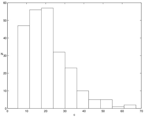
Figure 1: Histogram for $C$ - the degree of similarity of the results obtained by Dias and the accumulation method (11).

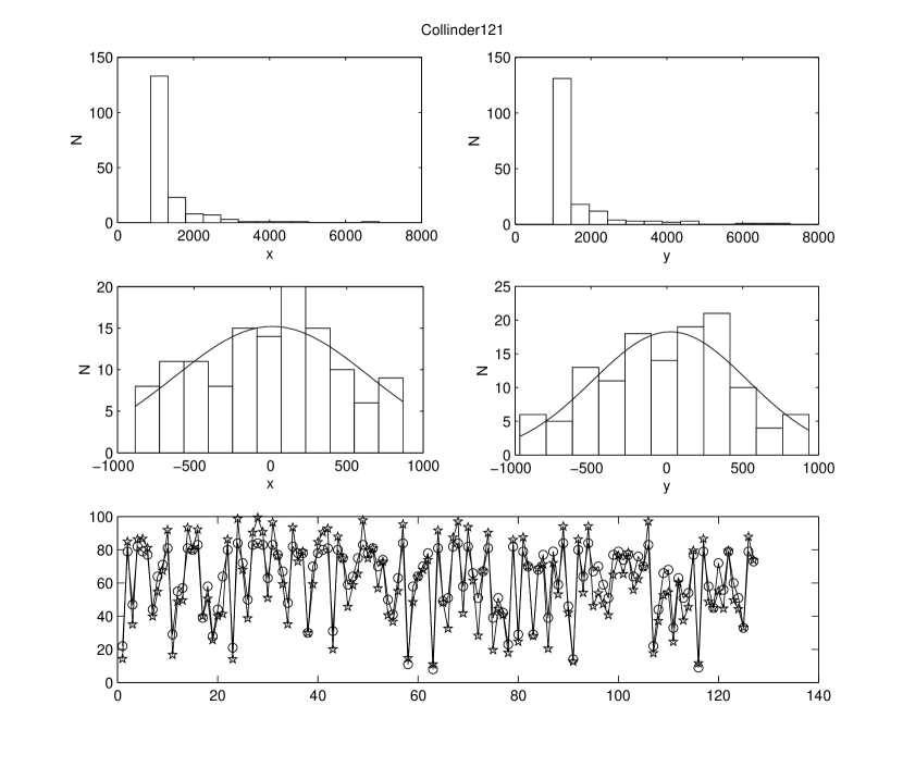
Figure 2: Collinder 121: the first row - the histograms for $|\delta\mu_{\alpha}|$ and $|\delta\mu_{\beta}|$ (formulae (9)); the second row - histograms for $\delta\mu_{\alpha}$ and $\delta\mu_{\beta}$ (formulae (10)); the third row - comparison of individual probabilities by Dias (circles) and by the accumulation method (asterisks)

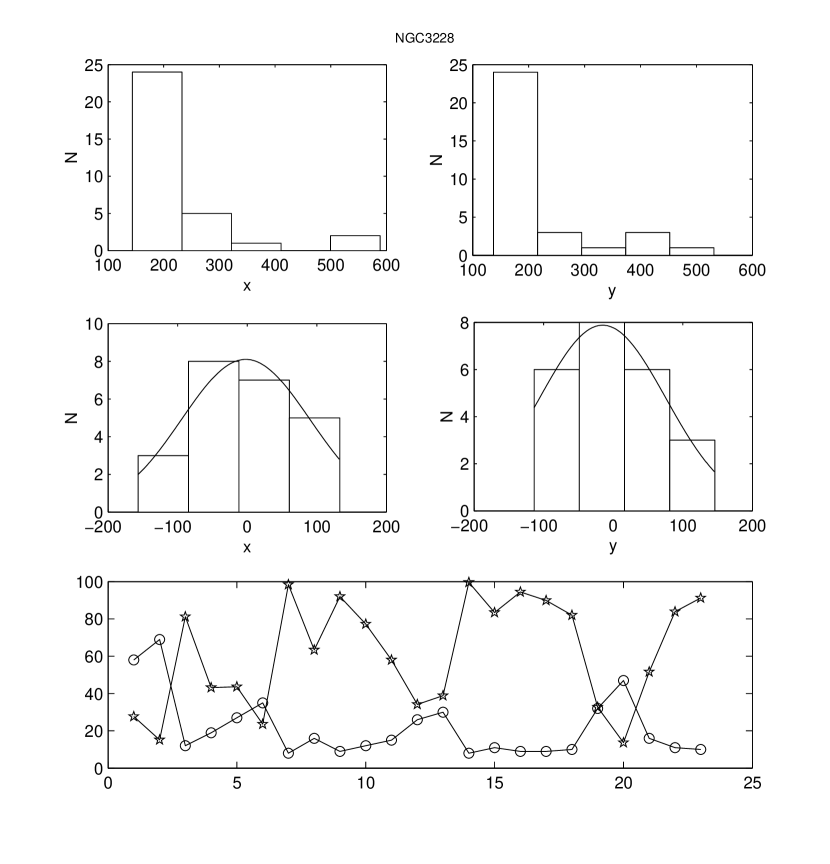
Figure 3: NGC3228: the first row - the histograms for $|\delta\mu_{\alpha}|$ and $|\delta\mu_{\beta}|$ (formulae (9)); the second row - histograms for $\delta\mu_{\alpha}$ and $\delta\mu_{\beta}$ (formulae (10)); the third row - comparison of individual probabilities by Dias (circles) and by the accumulation method (asterisks)

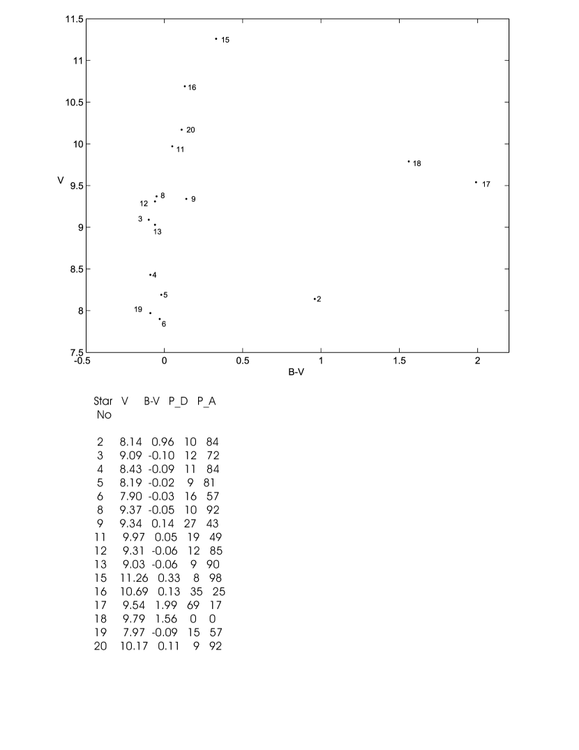
Figure 4: The color-magnitude diagram for NGC3228

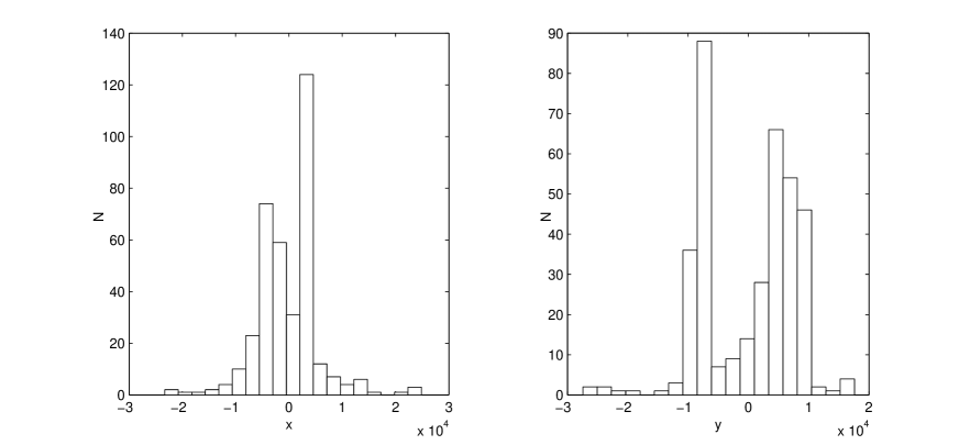
Figure 5: The Pleades (Mellotte22): histograms for $\delta\mu_{\alpha_{i}}$ (left) and $\delta\mu_{\delta_{i}}$ (right).

References

- (1) Sanders, W.L. 1971, A&A, 14, 226-232
- (2) Vasilevskis S., Klemola, A. & Preston, G. 1958, Ap.J. 63, 387
- (3) Slovak, M. 1977, Ap.J. 82, 10
- (4) Cabrera-Caño, J. & Alfaro, E.J. 1985 A&A 150, 298-301
- (5) McNamara, B.J. & Schneeberger, T.J. 1978, A &A 62, 449-451
- (6) Zhao, J.L. & He, Y.P. 1990, A &A 237, 54-60
- (7) Cabrera-Caño, J. & Alfaro, E.J. 1990, A &A 235, 94-102
- (8) Dias W. S., Lepine J. R. D., Alessi B. S., 2001, A &A 376, 441
- (9) Dias W. S., Lepine J. R. D., Alessi B. S., 2002, A &A 388, 168