Frustration of decoherence in $Y$-shaped superconducting Josephson networks

Abstract

We examine the possibility that pertinent impurities in a condensed matter system may help in designing quantum devices with enhanced coherent behaviors. For this purpose, we analyze a field theory model describing Y- shaped superconducting Josephson networks. We show that a new finite coupling stable infrared fixed point emerges in its phase diagram; we then explicitly evidence that, when engineered to operate near by this new fixed point, Y-shaped networks support two-level quantum systems, for which the entanglement with the environment is frustrated. We briefly address the potential relevance of this result for engineering finite-size superconducting devices with enhanced quantum coherence. Our approach uses boundary conformal field theory since it naturally allows for a field-theoretical treatment of the phase slips (instantons), describing the quantum tunneling between degenerate levels.

For engineering quantum devices one has often to tame the decoherence arising from the interaction of a pertinent two-level system with both the control circuitry and the quantum modes lying outside the subspace spanned by the two operating states. An important source of decoherence arises when the total state of the two-level system and of its environment evolve towards an entangled state. If a system is coupled to more than one bath, and its entanglement with each one of the baths is suppressed by the other(s), decoherence may be frustrated [1, 2]. In this paper, we evidence how frustration of decoherence may arise from the existence of a finite coupling fixed point (FFP) in the phase diagram of the quantum theory describing the device.

Existence of finite coupling fixed points in condensed matter is a rare instance realized, so far, only in quantum systems with pertinent impurities. Remarkable examples of systems exhibiting attractive FFP’s are provided by the two-channel single-impurity [3] and two-impurity [4] overscreened Kondo models, as well as by $Y$-shaped junction of quantum wires [5]. At variance, $Y$-shaped junctions of one-dimensional atomic condenstates [6] exhibit a repulsive FFP, signaling the existence of a new transition point between stable weakly and the strongly coupled phases.

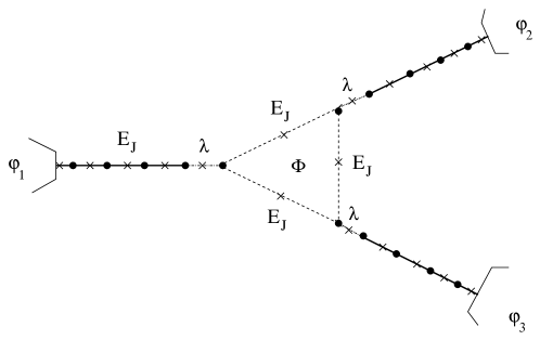
Figure 1: Sketch of the YJJN; Inset: graphical exact solutions for the energy levels at $g=9/8$.

Boundary conformal field theories [7] are a natural setting to investigate stable phases and phase transitions of quantum impurity systems, once the quantum impurity is traded [7] for a boundary interaction, involving only a subset of the bulk degrees of freedom: the boundary interaction is then renormalized by the bulk degrees of freedom, and the infrared (IR) behavior is determined by the stable fixed point(s) in the phase diagram.

Superconducting Josephson devices are not only promising candidates for realizing quantum coherent two-level systems [8], but also provide remarkable realizations of quantum systems with impurities, whose phase diagrams, in the simple cases so far investigated, admit only two fixed points: an unstable weak coupling fixed point (WFP), and a stable one at strong coupling (SFP) [9]. The approach developed in Ref.[9] naturally allows for a field-theoretical treatment of the phase slips describing quantum tunneling between degenerate levels, and provides remarkable analogies to models of quantum Brownian motion on frustrated planar lattices [10, 11]. When an effective two-level quantum system is operated near by the WFP or the SFP, there is no frustration of decoherence, since, at strong coupling, there is not even quantum tunneling between the degenerate states while, at weak coupling, there is full entanglement between the two degenerate states and the plasmon modes. In the following, we shall show that a FFP emerges in a $Y$-shaped Josephson junction network (YJJN), and that it may be pertinently used to engineer two-level systems with enhanced quantum coherence.

A YJJN is realized by joining a circular Josephson junction array C to three finite Josephson chains via weak links of nominal strength $\lambda$ (see Fig.1). C is pierced by a dimensionless magnetic flux $\Phi$, and is joined to one of the endpoints of the three chains (inner boundary); the other endpoints (outer boundary) are connected to three bulk superconductors at fixed phases $\varphi_{i}$ ($i=1,2,3$). For simplicity, we assume that all the junctions in the YJJN are of strength $E_{J}$ and that $\lambda\ll E_{J}$. The Hamiltonian describing C is given by

$$H_{\bf C}=\frac{E_{c}}{2}\sum_{i=1}^{3}\left[-i\frac{\partial}{\partial\phi_{0}^{(i)}}-W_{g}\right]^{2}-2E_{J}\sum_{i=1}^{3}\cos\left[\Delta\phi_{0}^{(i)}+\frac{\Phi}{3}\right]\;\;\;\;,$$ (1)

where $\Delta\phi_{0}^{(i)}=\phi_{0}^{(i)}-\phi_{0}^{(i+1)}$, $\phi_{0}^{(i)}$ is the phase of the superconducting order parameter at grain $i$, and $W_{g}$ is a gate voltage. If $E_{J}/E_{c}\ll 1$, $W_{g}^{(i)}=N+\frac{1}{2}+h$, with integer $N$ and $0<h<1/2$, the low-energy dynamics is governed only by the two states with total charge equal to $N$ and to $N+1$.

The procedure outlined in Ref.[9] allows to describe the three finite chains with a Tomonaga-Luttinger Hamiltonian

$$H_{0}=\frac{g}{4\pi}\sum_{i=1}^{3}\>\int_{0}^{L}\>dx\>\left[\frac{1}{v}\left(\frac{\partial\Phi_{i}}{\partial t}\right)^{2}+v\left(\frac{\partial\Phi_{i}}{\partial x}\right)^{2}\right]\>\>\>\>.$$ (2)

In Eq.(2) $\Phi_{i}$ describe the plasmon modes of the chains, and $g$ and $v$ depend on the constructive parameters of the network [9].

Fixing the phase at the outer boundary of the chains sets Dirichlet boundary conditions on $\Phi_{i}(x)$ at $x=L$: $\Phi_{i}(L)=\varphi_{i}$. Since we require that the charge tunneling between ${\bf C}$ and the inner boundary of the three chains is described by a Josephson-like interaction, with nominal strength $\lambda\ll E_{J}$, one should use Neumann boundary conditions at the inner boundary, i.e. $\frac{\partial\Phi_{i}(0)}{\partial x}=0$ $\forall i$. This allows to write the tunneling Hamiltonian as $H_{T}=-\lambda\sum_{i=1}^{3}\cos[\Phi_{i}(0)-\phi_{0}^{(i)}]$.

A boundary field theory approach allows to trade $H_{\bf C}+H_{T}$ with an effective boundary Hamiltonian, $H_{b}$, involving only $\Phi_{i}(0)$, and given by

$$H_{b}=-2\bar{E}_{W}\sum_{i=1}^{3}:\cos[\vec{\alpha}_{i}\cdot\vec{\chi}(0)+\gamma]:\;\;\;\;,$$ (3)

with $\chi_{1}(x)=\frac{1}{\sqrt{2}}[\Phi_{1}(x)-\Phi_{2}(x)]$, $\chi_{2}(x)=\frac{1}{\sqrt{6}}[\Phi_{1}(x)+\Phi_{2}(x)-2\Phi_{3}(x)]$, $\vec{\alpha}_{1}=(1,0)$, $\vec{\alpha}_{2}=(-\frac{1}{2},\frac{\sqrt{3}}{2})$, $\vec{\alpha}_{3}=(-\frac{1}{2},-\frac{\sqrt{3}}{2})$, $\gamma=\tan^{-1}[3\tan(\frac{\Phi}{3})]$, and $\bar{E}_{W}=\left(\frac{a}{L}\right)^{\frac{1}{g}}E_{W}$, with $E_{W}\approx\frac{\lambda^{2}E_{J}}{24(E_{c})^{2}\tilde{h}^{2}}\sqrt{1+2\sin^{2}(\frac{\Phi}{3})}$. The colons $:\>:$ denote normal ordering with respect to the ground state of the plasmon modes, $|\{0\}\rangle$. In the following, we shall argue that, for $\gamma=\pi/3$, there is a finite range of values of $g$, for which a YJJN supports a FFP: this results from the fact that, for this value of $\gamma$, the two plasmon baths $\chi_{1}$ and $\chi_{2}$, cooperate to destabilize both the SFP and the WFP.

The perturbative second-order renormalization group (RG) equation for the running coupling strength $G=L\bar{E}_{W}$, given by

$$\frac{dG}{d\ln(\frac{L}{L_{0}})}=\left(1-\frac{1}{g}\right)G-2G^{2}\>\>\>\>,$$ (4)

shows that $H_{b}$ is a relevant perturbation for $g>1$, while it is irrelevant for $g<1$. In Eq.(4), $L_{0}$ is a pertinent reference length scale. The strongly coupled fixed point (SFP) is reached when the running coupling constant $G$ goes to $\infty$. The fields $\chi_{j}(x)$, $j=1,2$, now obey Dirichlet boundary conditions at $x=0$ and $\chi_{1}(0),\chi_{2}(0)$ are determined by the manifold of the minima of the effective boundary potential (Eq.(3)). One sees that for $0\leq\gamma<\pi/3$, the minima lie on the triangular sublattice A, defined by $(\chi_{1}(0),\chi_{2}(0))=(2\pi m_{12},\frac{2}{\sqrt{3}}[2\pi m_{13}+\pi m_{12}])$, while, for $\pi/3<\gamma\leq 2\pi/3$, the minima lie on the triangular sublattice B, given by $(\chi_{1}(0),\chi_{2}(0))=(2\pi m_{12}-\frac{2\pi}{3},\frac{2}{\sqrt{3}}[2\pi m_{13}+\pi m_{12}-\pi])$, with $m_{12},m_{13}$ relative integers. From Eq.(3), one sees also that the difference in energy between the sets of the minima forming the A and B sublattices is given by $\sim\bar{E}_{J}\sin(\gamma-\frac{\pi}{3})$. The manifold of the minima is depicted in Fig.2, where the instanton connecting the degenerate minima of the honeycomb lattice emerging when the A and B sublattices are degenerate, is shown.

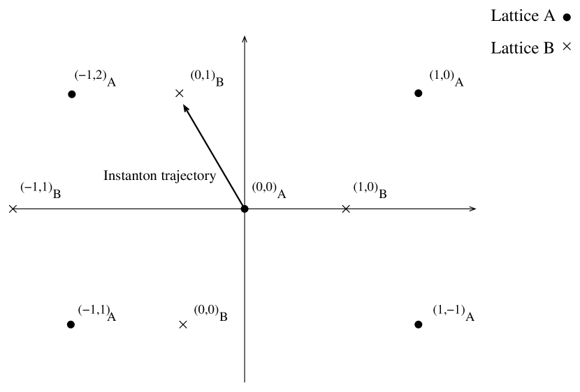
Figure 2: Some points on the two lattices A and B: at $\gamma=\pi/3$, the two lattices are degenerate. In this case, the set of the minima of the boundary potential spans a honeycomb lattice, whose sites are connected by instanton trajectories as the one drawn in the figure.

Following the approach outlined in Ref.[10], instanton effects may be taken into account through

$$\tilde{H}_{b}=-Y\sum_{i=1}^{3}\{T^{-}V_{i}(0)+T^{+}\bar{V}_{i}(0)\}\>\>\>\>.$$ (5)

In Eq.(5), $\vec{T}$ is an effective isospin operator, connecting two neighboring minima of the honeycomb lattice of the zero-mode eigenvalues, $V_{i}(\bar{V}_{i})=:\exp\left[-(+)\frac{2}{3}\vec{\alpha}_{i}\cdot\vec{\Theta}\right]:$, with $\vec{\Theta}$ being the dual fields of $\vec{\chi}$, while $\tilde{H}_{b}$ is the ”dual” boundary Hamiltonian of Eq.(3). $Y$ is an effective coupling defined as $Y=E_{J}-\bar{E}_{W}$ [12]. From the O.P.E. of the vertex operators entering $\tilde{H}_{b}$, the RG equation for the running coupling strength $y=LY$ is

$$\frac{dy}{d\ln\left(\frac{L}{L_{0}}\right)}=\left(1-\frac{4g}{9}\right)y-\frac{2g}{3}y^{3}\>\>\>\>.$$ (6)

For $\gamma=\pi/3$ and $1<g<\frac{9}{4}$, neither the WFP, or the SFP, are stable. Accordingly, a minimal hypothesis for the phase diagram requires a FFP at $y=y_{*}$, with $y_{*}$ finite. For instance, for $g=\frac{9}{4}-\epsilon$, with $\epsilon\ll 1$, one obtains $y^{*}\approx\left(\frac{2}{3}\right)^{\frac{1}{2}}\sqrt{\epsilon}$.

The energy of the minima may be varied by changing the phases of the three bulk superconductors since the eigenvalues $(p_{1},p_{2})$ of the zero-modes of the fields $\chi_{j}$ (it obeys Dirichlet b.c.!) depend on the phases $\varphi_{j}$ as

$$(p_{1},p_{2})=\sqrt{\frac{g}{2}}(n_{1}+\sqrt{2}\beta_{1},\frac{1}{\sqrt{3}}(2n_{2}+n_{1}+2\sqrt{2}\beta_{2}))\>\>\>\>,$$ (7)

on sublattice A, and

$$(p_{1},p_{2})=\sqrt{\frac{g}{2}}(n_{1}-\frac{1}{3}+\sqrt{2}\beta_{1},\frac{1}{\sqrt{3}}(2n_{2}+n_{1}-1+2\sqrt{2}\beta_{2}))\>\>\>\>,$$ (8)

on sublattice B. In Eqs.(7,8) $(n_{1},n_{2})$ are integers, $\beta_{1}=(\varphi_{1}-\varphi_{2})/(2\pi\sqrt{2})$, and $\beta_{2}=(\varphi_{1}+\varphi_{2}-2\varphi_{3})/(2\pi\sqrt{6})$.

As it happens with other superconducting systems [8], also a YJJN supports a two-level quantum system, operating between two pertinently selected quantum states. Indeed, for $y\ll 1$ and near the SFP, the low-energy spectrum is given by $E=\frac{\pi v}{2L}[\vec{p}]^{2}+E^{\prime}$, where $\vec{p}=(p_{1},p_{2})$ labels the zero-mode contribution, while $E^{\prime}$ comes from the plasmon modes: thus, for $\gamma=\pi/3$, a pertinent tuning of $\beta_{1}$ and $\beta_{2}$ renders degenerate the zero-mode contributions to the total energy coming from two nearest neighboring sites of the honeycomb lattice resulting from the degeneracy of the A and B sublattices (see Fig.2). This happens, for instance, if $\beta_{1}=1/3\sqrt{2},\beta_{2}=0$: the two degenerate quantum states $|\uparrow\rangle$ and $|\downarrow\rangle$ -labelled by $(n_{1},n_{2})=(0,0)$ on sublattice A and by $(n_{1},n_{2})=(1,0)$ on sublattice B- are macroscopically characterized by the opposite values of the Josephson current flowing across chain-1 and chain-2, namely: $I_{1}=-I_{2}=\pm\frac{\pi gve^{*}}{3L}$, $I_{3}=0$.

Quantum tunneling between the degenerate states is induced by $\tilde{H}_{b}$, with matrix element $-Y$. Setting $\beta_{2}=0$, and $\beta_{1}=1/3\sqrt{2}+\delta/(2\pi)$, with $\delta/2\pi\ll 1$, one easily gets an effective Hamiltonian for the two-level quantum system as

$$H_{2}=\epsilon_{0}(\delta){\bf I}+\epsilon(\delta)\sigma^{z}-Y\sigma^{+}\bar{V}_{1}(0)-Y\sigma^{-}V_{1}(0)\;\;\;\;.$$ (9)

In Eq.(9) $\epsilon_{0}(\delta)=\frac{g}{2}\left(\frac{1}{9}+\frac{\delta^{2}}{4\pi^{2}}\right)$, $\epsilon(\delta)=\frac{g}{3}\frac{\delta}{\sqrt{2}\pi}$, the $\sigma^{a}$’s are the Pauli matrices, $\delta$ is a control parameter determined by the phases $\{\varphi_{i}\}$, and $-Y[\sigma^{+}\bar{V}_{1}(0)+\sigma^{-}V_{1}(0)]$ describes the interaction of the two-level system with the phase slip operators introduced in Eq.(5)

In the spin Hamiltonian describing the two level system in Eq.(9), one sees that there is a $z$-component proportional to $\epsilon(\delta)$, as well as an $x$-component proportional to $Y$. While $\epsilon(\delta)$ does not get renormalized by the interaction with the two plasmon fields, $Y$ is renormalized and its value measures the amount of entanglement between the two-level system and the plasmon modes bath. In particular, if $Y$ is irrelevant, the two-level system decouples from the environment and behaves as a classical (Ising-like) spin, pointing along $z$. When this happens, no energy is dissipated into the environment, and the spectrum of the Hamiltonian in Eq.(9) is given by two classical states with $\omega=\pm\epsilon(\delta)$. If $Y\to\infty$, the effective field acting on the two-level system would again make it behave as a classical spin, pointing in the $x$-direction: now, all the energy is dissipated into the environment and the spectrum of Eq.(9) is given by only an overdamped mode at $\omega=0$. Only when $Y$ takes a finite value $y_{*}$, the competition between $\epsilon(\delta)$ and $y_{*}$ may lead to the emergenge of the frustration of the decoherence of the two-level system, since there is the possibility that, for a pertinent choice of the control parameter $\epsilon(\delta)$, there is a finite damping, resulting in two broad modes, centered at pertinent renormalized energies.

To evidence the frustration of decoherence around the FFP, we compute the spectral density of the Hamiltonian in Eq.(9), given by $\chi^{``}_{\perp}(\omega)/\omega$, where $\chi^{``}_{\perp}(\omega)$ is the imaginary part of the transverse dynamical spin susceptibility [1]. The diagrams contributing to $\chi_{\perp}(\omega)$ are shown in Fig.(3 b): $\chi_{\perp}(\omega)$ is computed as a loop defined by the $|\uparrow\rangle$-state propagating forward in (imaginary) time, and by the $|\downarrow\rangle$-state propagating backward. It is given by

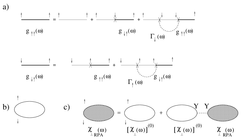
Figure 3: a): Graphical representation for the Schwinger-Dyson equations for $g_{\sigma\sigma^{\prime}}(\omega)$; b): The “bubble” yielding the dynamical spin susceptibility; c): Graphical representation of the RPA summation implemented to compute $\chi_{\perp}(\omega)$ near the FFP.

$$\chi_{\perp}(\omega)=-i\int_{-\infty}^{\infty}\;\frac{dz}{2\pi}\{g_{\uparrow,\uparrow}^{*}(-z)g_{\downarrow,\downarrow}(z+\omega)+g_{\downarrow,\downarrow}^{*}(-z)g_{\uparrow,\uparrow}(z+\omega)\}\>\>\>\>,$$ (10)

where $g_{\sigma\sigma}(\omega)$ is the Fourier tranform of the propagator of the “spin” eigenstate $|\sigma\rangle$ ($\sigma=\uparrow,\downarrow$).

For $\gamma=\pi/3$ and $g>9/4$, the boundary interaction is irrelevant, and one may neglect corrections to the amplitudes of order $Y^{2}$. This amounts to substituting $g_{\sigma\sigma}(\omega)$ with its noninteracting limit, $g^{(0)}_{\sigma}(\omega)=1/[i\omega+\sigma\epsilon(\delta)]$, yielding

$$\frac{\chi^{"}(\omega)}{\omega}\propto[\delta(\omega+2\epsilon(\delta))-\delta(\omega-2\epsilon(\delta))]/\omega\>\>\>\>.$$ (11)

Eq.(11) shows that there is no entanglement (for $g>9/4$) between the two-level quantum system and the plasmon modes. Since, in this range of $g$, there is no tunnel splitting between the two degenerate states, the system is classical and no quantum coherence emerges.

For $\gamma=\pi/3$ and $g<1$, instantons provide a relevant perturbation and the IR behavior of the system is driven by the WFP. To compute $\chi_{\perp}(\omega)$, one now needs to substitute $g^{(0)}_{\sigma}(\omega)$ with the dressed propagator, $g_{\sigma\sigma}(\omega)$, drawn in Fig.(3 a), where the solid heavy line represents the fully dressed propagator, while the solid light line represents $g_{\sigma}^{(0)}(\omega)$. As a result, $g_{\sigma\sigma^{\prime}}(\omega)$ is given by

$$g_{\sigma,\sigma^{\prime}}(\omega)=\frac{\delta_{\sigma,\sigma^{\prime}}[[g^{(0)}_{\bar{\sigma}}]^{-1}(\omega)+Y^{2}\Gamma_{\sigma}(\omega)]+iY\delta_{\sigma,{\bar{\sigma}}{{}^{\prime}}}}{\{[g^{(0)}_{\uparrow}]^{-1}(\omega)+Y^{2}\Gamma_{\downarrow}(\omega)\}\{[g^{(0)}_{\downarrow}]^{-1}(\omega)+Y^{2}\Gamma_{\uparrow}(\omega)\}+Y^{2}}\>\>\>\>,$$ (12)

with $\bar{\sigma}=-\sigma$, and $\Gamma_{\sigma}(\omega)$ is the Fourier transform of the propagation function

$$\Gamma(\tau_{1}-\tau_{2})=\langle\{0\}|:e^{\pm i\frac{2}{3}\Theta(\tau_{1})}::e^{\mp i\frac{2}{3}\Theta(\tau_{1})}:|\{0\}\rangle=[e^{\frac{\pi i}{L}v\tau_{1}}-e^{\frac{\pi i}{L}v(\tau_{2}+i\eta)}]^{-\frac{8}{9}g}\>\>\>\>,$$ (13)

at frequency $\omega-\sigma\epsilon(\delta)$. $\chi_{\perp}(\omega)$ near the WFP is computed by taking the large-$Y$ limit of Eq.(12), yielding

$$\frac{\chi^{"}(\omega)}{\omega}\propto[|2\epsilon(\delta)+\omega|^{3-\frac{16}{9}g}-|2\epsilon(\delta)-\omega|^{3-\frac{16}{9}g}]/\omega\>\>\>\>.$$ (14)

Eq.(14) shows that a large part of the spectral weight has moved now from the side peaks towards $\omega=0$, signaling the strong decoherence of the two-level system described by Eq.(9).

For $\gamma=\pi/3$ and $1<g<\frac{9}{4}$, the IR behavior is driven by the FFP. A closed-form computation of $\chi_{\perp}(\omega)$ is now possible only for special values of $g$. For instance, if $g=\frac{9}{4}-\epsilon$ with $\epsilon\ll 1$, $y_{*}$ is $\ll 1$, and one may compute $\chi_{\perp}(\omega)$ by resorting to a RPA summation, graphically sketched in Fig.(3c)). The result is

$$[\chi_{\perp}]_{\rm RPA}(\omega)\approx\frac{1}{\omega-2\sqrt{\epsilon^{2}(\delta)+Y^{2}}-Y^{2}\Gamma[-1-\frac{8}{9}\gamma](-\omega)^{1+\frac{8}{9}\gamma}}$$

$$+\frac{1}{\omega+2\sqrt{\epsilon^{2}(\delta)+Y^{2}}-Y^{2}\Gamma[-1-\frac{8}{9}\gamma](-\omega)^{1+\frac{8}{9}\gamma}}\>\>\>\>.$$ (15)

When writing $[\chi_{\perp}]_{\rm RPA}(\omega)$ as a function of the dimensionless variable $x=\frac{2L}{\pi v}\omega$, taking into account that the dimensionless variable $y=YL^{1-\frac{4}{9}g}\longrightarrow y_{*}$ as $L\to\infty$, one gets

$$[\chi_{\perp}]_{\rm RPA}(x)\propto\frac{1}{x-2\Delta+e^{i\pi\frac{8}{9}\gamma}x^{1+\frac{8}{9}\gamma}}+\frac{1}{x+2\Delta+e^{i\pi\frac{8}{9}\gamma}x^{1+\frac{8}{9}\gamma}}\>\>\>\>,$$ (16)

where $\Delta=\frac{2L}{\pi v}\sqrt{E^{2}+Y^{2}}$. The imaginary part of Eq.(16) shows two peaks centered around $\pm 2\sqrt{[\epsilon(\delta)]^{2}+(\frac{\pi v}{L}y_{*})^{2}}$, where $y_{*}$ is the finite fixed point value of the running coupling constant. In Fig.4, we provide the plot of $\chi^{``}(\omega)/\omega$.

A very special situation arises for $\gamma=\pi/3$ when $g=9/8$ since, for this value of $g$, the scaling dimension of the relevant instanton operators equals 1/2, just as it happens with fermionic operators. Indeed, for $g=9/8$, the plasmon field $:\exp\left[-\frac{2}{3}i\sqrt{2g}\Theta(x,\tau)\right]:$ becomes a fermionic operator $\psi(x+iv\tau)$ ($-L\leq x\leq L$), and the spin-1/2 operators may be fermionized according to

$$\sigma^{z}\longrightarrow a^{\dagger}a-\frac{1}{2}\;\;\;,\;\;\sigma^{+}\longrightarrow a^{\dagger}e^{\frac{3}{2}i\pi\sqrt{\frac{2}{g}}P_{1}}\;\;\;\;,$$ (17)

where the zero-mode operator $P_{1}$ ensures, for $g=9/8$, the correct anticommutation relations between $\psi$ and the operators in Eq.(17). As a result, the two-level Hamiltonian Eq.(9) becomes

$$H_{\rm Fer}=-iv\int_{-L}^{L}\>dx\>\psi^{\dagger}(x)\frac{\partial\psi(x)}{\partial x}+\epsilon(\delta)(a^{\dagger}a-\frac{1}{2})-Y\psi(0)a^{\dagger}e^{\frac{3}{2}i\pi\sqrt{\frac{2}{g}}P_{1}}-{\rm h.c.}\>\>\>\>,$$ (18)

with twisted boundary condition

$$\psi(L)=\exp\left[\frac{4}{3}i\pi\sqrt{g}p_{1}\right]\>\psi(-L)\>\>\>\>,$$ (19)

where $p_{1}$ is the eigenvalue of the zero-mode operator $P_{1}$. A similar situation arises in the analysis of a spin-1/2 Kondo system at the Toulouse point [13]. In particular, the Hamiltonian in Eq.(18) has been recently proposed [14] to describe two qubits at the end of a finite length 1d cavity.

To determine the energy eigenstates of the Hamiltonian in Eq.(18), $|E\rangle$, with the boundary condition in Eq.(19), one may posit

$$|E\rangle=\left\{\int_{-L}^{L}\>dx\>f_{E}(x)\psi^{\dagger}(x)+\lambda_{E}a^{\dagger}\right\}|{\bf 0}\rangle\>\>\>\>,$$ (20)

where $|{\bf 0}\rangle$ is the simultaneous eigenstate of $P_{1}$ and $\sigma^{z}$ given by $|(p_{1}=-\sqrt{\frac{g}{2}}\frac{\delta_{1}}{2\pi}),\downarrow\rangle$. From $H_{\rm Fer}|E\rangle=E|E\rangle$, one gets

$$-iv\frac{\partial f_{E}(x)}{\partial x}+Y\lambda_{E}e^{\frac{3}{4}i\delta_{1}}\delta(x)=Ef_{E}(x)$$

$$\lambda_{E}\epsilon(\delta)+Yf_{E}(0)e^{-\frac{3}{4}i\delta_{1}}=E\lambda_{E}\>\>\>\>,$$ (21)

which is solved by

$$f_{E}(x)=\frac{1}{\sqrt{2L}}[e^{i\frac{\chi}{v}}\theta(x)+e^{-i\frac{\chi}{v}}\theta(-x)]\>\>\>\>,$$ (22)

provided that

$$\frac{E}{v}L+\frac{\chi}{v}+\frac{\pi}{2}=0\>\>\>;\;\;v\tan\left(\frac{\chi}{v}\right)+L\frac{Y^{2}}{E-\epsilon(\delta)}=0\;\;\;\;.$$ (23)

In the inset of Fig.1, Eqs.(23) are graphically solved for $\epsilon(\delta)=0$, using the dimensionless variable $x=LE/v$.

For $g>1$, inhomogeneities in the fabrication parameter $E_{J}$ provide an irrelevant perturbation, since the pertinent operator scales as $\left(\frac{L}{L_{0}}\right)^{1-g}$ [9] and, thus, does not alter the main results of our analysis. Furthermore, today ’s technology allows to fabricate superconducting devices with values of $g$ ranging from $g<1$, to $g\sim 2$ [15].

Operating a YJJN near the FFP allows to engineer a realistic finite-size two-level quantum device with enhanced quantum coherence. Indeed, for a YJJN of finite size $L$, the FFP is stable against small fluctuations of the flux $\Phi$, provided that $v/L$ is sufficiently big: if $\gamma=\pi/3$ is displaced by a small amount $\nu$, $v/L$ needs to be larger than the energy splitting $\bar{E}_{W}\sin(\nu)$ between the minima of the two triangular sublattices. When $v/L<\bar{E}_{W}\sin(\nu)$, there is a flow towards the SFP and, depending on ${\rm sgn}(\nu)$, the minima of the boundary potential lie on either one of the triangular A and B sublattices (see Fig.5). The parameters $\beta_{1},\beta_{2}$ may be safely tuned to the degeneracy values $\beta_{1}=1/(3\sqrt{2})$, $\beta_{2}=0$ by resorting to multipolar magnetic coils [16] inserted in loops connecting the bulk superconductors at the outer boundary of the YJJN since, for sufficiently long chains, the magnetic flux generated by the coil does not alter the flux threading the circular Josephson junction array C.

Josephson networks where $n$ finite chains are connected to a central circular array ${\bf C}$ share properties similar to a YJJN. For $n=4$, the resulting network is the tetrahedral qubit proposed in Ref.[17].

In summary, our analysis of YJJNs provides an explicit example of a situation in which quantum impurities may be pertinently used for engineering quantum devices with enhanced quantum coherence.

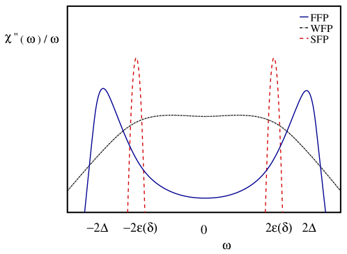
Figure 4: Qualitative behavior of $\chi^{"}(\omega)/\omega$ in the various regimes.

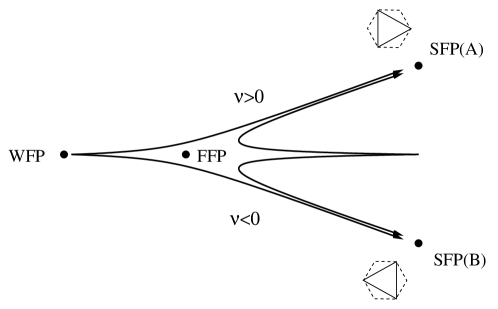
Figure 5: Sketch of the RG flow for $\gamma=\pi/3+\nu$ ($\nu/\pi\ll 1$).

We thank I. Affleck, C. Chamon, P. Degiovanni, R. Russo and A. Trombettoni for useful discussions and correspondence.

References

References

- [1] A. H. Castro Neto, E. Novais, L. Borda, G. Zaránd, and I. Affleck, Phys. Rev. Lett. 91, (2003) 096401-1; E. Novais, A. H. Castro Neto, L. Borda, I. Affleck, and G. Zarand, Phys. Rev. B 72, (2005), 014417.
- [2] H. Kohler and F. Sols, New J. Phys. 8, (2006), 149.
- [3] P. Nozières and A. Blandin, J. Phisique 41, (1980), 193.
- [4] I. Affleck, A. W. W. Ludwig, and B. Jones, Phys. Rev. B 52, (1995), 9528.
- [5] C. Chamon, M. Oshikawa and I. Affleck, Phys. Rev. Lett. 91, (2003), 206403; M. Oshikawa, C. Chamon and I. Affleck, Journal of Statistical Mechanics JSTAT/2006/P02008; Chang-Yu Hou and Claudio Chamon, Phys. Rev. B 77, (2008), 155422.
- [6] A. Tokuno, M. Oshikawa and E. Demler, Phys. Rev. Lett. 100, (2008), 140402.
- [7] J. Cardy, Encyclopedia of Mathematical Physics, (Elsevier, 2006) (physics arXiv:hep-th/0411189).
- [8] Y. Makhlin, G. Shön, and A. Shnirman, Rev. Mod. Phys. 73, (2001), 357.
- [9] D. Giuliano and P. Sodano, Nucl. Phys. B 711, (2005), 480; Nucl. Phys. B 770, (2007), 332.
- [10] H.Yi and C.L.Kane, Phys.Rev.B 57,R5579-R5582(1998).
- [11] I. Affleck, M. Oshikawa and H. Saleur, Nucl. Phys. B594, (2001), 535.
- [12] A. M. Tsvelik, ”Quantum Field Theory in Condensed Matter Physics”, Cambridge University Press, Cambridge, UK (Chapter 29).
- [13] V. J. Emery and S. Kivelson, Phys. Rev. Lett. 67 1991 (2882); Phys. Rev. B 46, (1992), 10812.
- [14] S. Camalet, J. Schriefl, P. Degiovanni, F. Delduc, Europhysics Letters 68, (2004) 37.
- [15] D. B. Haviland, K. Andersson, and P. Agren, J. Low Temp. Phys. 124,(2001) 291.
- [16] C. Granata, A. Vettoliere and M. Russo, Appl. Phys. Lett. 88, (2006) 212506.
- [17] M. V. Feigel’man, L. B. Ioffe, V. B. Geshkenbern, P. Dayal, and G. Blatter, Phys. Rev. Lett 92, 098301 (2004); Phys. Rev. B 70, 224524 (2004).