Linear Response and Stability of Ordered Phases of Block Copolymer Melts

Abstract

An efficient pseudo-spectral numerical method is introduced for calculating a self-consistent field (SCF) approximation for the linear susceptibility of ordered phases in block copolymer melts (sometimes referred to as the random phase approximation). Our method is significantly more efficient than that used in the first calculations of this quantity by Shi, Laradji and coworkers, allowing for the study of more strongly segregated structures. We have re-examined the stability of several phases of diblock copolymer melts, and find that some conclusions of Laradji et al. regarding the stability of the Gyroid phase were the result of insufficient spatial resolution. We find that an epitaxial (${\bf k}=0$) instability of the Gyroid phase with respect to the hexagonal phase that was considered previously by Matsen competes extremely closely with an instability that occurs at a nonzero crystal wavevector ${\bf k}$.

I Introduction

The local stability of periodic structures, such as those formed by block copolymer melts, may be characterized by a linear response function that describes the nonlocal response of the monomer concentrations to a hypothetical external chemical potential field. This response function is closely related to the correlation function that is probed by small angle x-ray and neutron scattering. The use of a self-consistent field (SCF) approximation to calculate the linear susceptibility of a homogeneous polymer blend or disordered diblock copolymer melt is often referred as a “random phase approximation” (RPA) for the correlation function.¹ This usage has become entrenched in the polymer literature, despite its somewhat obscure origin ^{2, 3, 4} as one of several names for the use of a time-dependent SCF theory (i.e., time-dependent Hartree theory) to calculate the dynamic linear response of a free electron gas ⁵, ⁶.

In this paper, we present an efficient numerical method to calculate the SCF linear susceptibility of ordered phases of block copolymers. The SCF susceptibility of the disordered phase of a diblock copolymer melt was first calculated by Leibler ⁷. Leibler used this both to describe diffuse scattering from the disordered phase, and as one building block in his theory of weak microphase segregation. Shi, Laradji and coworkers ⁸, ⁹, ¹⁰ were the first to calculate the SCF susceptibility of ordered phases of diblock copolymer melts, which they used to examine the limits of local stability of various ordered structures.

The calculation of the full linear response for an ordered structure is a numerically intensive task. Laradji et al. ⁸, ⁹, ¹⁰ used a spectral method to complete this calculation that was closely analogous to the algorithm used by Matsen and Schick ¹¹ to study equilibrium structures. When applied to three dimensionally periodic structures such as the BCC and Gyroid phases, this algorithm was able to accurately describe only very weakly segregated structures. This limitation was a result of a rapid increase in computational cost with increases in the number $M$ of spatial degrees of freedom required to resolve the structure: The computational cost of a spectral calculation of the response to a single perturbation (e.g., the response to a single plane wave) is of ${\cal O}(M^{3})$, while the cost of a calculation of the full RPA response function (i.e., the response to an arbitrary small perturbation) is ${\cal O}(M^{4})$.

The earlier use of a spectral method by Matsen and Schick¹¹ to calculate the equilibrium phase diagram for diblock copolymer melts relied heavily upon the use of space group symmetry to decrease the number of basis function needed to describe a structure. Matsen and Schick introduced the use of basis functions with the space group symmetry of each structure of interest. Use of these symmetry-adapted basis functions functions reduces the number of degrees of freedom $M$ needed to obtain a given spatial resolution by a factor roughly equal to the number of point group symmetries in the relevant space group. For the BCC and Gyroid cubic phases, this reduces $M$ by almost a factor of 48, and thus reduced the cost of solution a single iteration of the SCF equations by a factor of almost $(48)^{3}\approx 10^{5}$.

The calculation of the full linear susceptibility, however, requires the calculation of the response to arbitrary infinitesimal perturbations, which generally do not preserve the space group symmetry of the crystal. In general, it thus requires the use of either a plane wave basis or a spatial discretization that does not impose any symmetry upon the perturbation. Primarily as a result of this loss of the advantages of symmetry, Laradji et al.^{9, 10} were able to obtain results for the Gyroid phase only for $\chi N\leq 12$. Matsen has been able to carry out linear response calculations for the BCC and Gyroid phases at significantly larger values of $\chi N$ by considering only the response to perturbations that preserve the periodicity of the cubic lattice, and that preserve a subgroup of the space group of the unperturbed structure ^{12, 13}. Matsen’s method and results are discussed in more detail in Sec. VII.

More recent work on numerical methods for solving the equilibrium SCFT by Rasmussen and Kalosakas ¹⁴, and by Fredrickson and co-workers ^{15, 16, 17} has made use of pseudo-spectral methods for which the cost of a single iteration of the SCFT equations scales as ${\cal O}(M\ln M)$, rather than ${\cal O}(M^{3})$. Here, we present a derivation of a perturbation theory for the linear response to an arbitrary disturbance in a form that we can evaluate numerically using a pseudo-spectral algorithm.

The remainder of the paper is organized as follows: In Section II, we discuss the basic formalism of the SCF linear response theory for perturbations of a periodic microstructure, and review the consequences of Bloch’s theorem. In Section III, we present a perturbation theory for the underlying modified diffusion equation, which is used to calculate the linear susceptibility of a reference system of non-interacting polymers in a periodic potential. In Section IV, we discuss the use of linearized SCFT to calculate the corresponding susceptibility of an incompressible system of interacting chains. In Section VI, we discuss the implementation and efficiency of our algorithm. Section VII presents selected results regarding the stability of the HEX, BCC, and (particularly) the Gyroid phases of diblock copolymer melts.

II Response of a periodic structure

In self-consistent field theory, we calculate the average concentration $\rho_{i}({\bf r})$ for monomers of type $i$ by considering a hypothetical system of non-interacting polymers in which monomers of type $i$ are subjected to a self-consistently determined field $\omega_{i}({\bf r})$. We consider incompressible systems in which each monomer occupies a volume $v$, and define a volume fraction field $\phi_{j}({\bf r})\equiv v\rho_{j}({\bf r})$.

In what follows, we consider the response of an unperturbed state in which $\omega_{i}({\bf r})$ satisfies the self-consistent field (SCF) equation

$$\omega_{i}({\bf r})=\chi_{ij}\phi_{j}({\bf r})+\xi({\bf r})\quad.$$ (1)

Here, $\chi_{ij}$ is a Flory-Huggins parameter for binary interactions between monomers of types $i$ and $j$, and $\xi({\bf r})$ is a Lagrange multiplier field that must be chosen so as to satisfy an incompressibility constraint. To calculate the SCF linear susceptibility, we consider the perturbation caused by an additional infinitesimal external potential $\delta\omega^{\rm ext}_{i}({\bf r})$. The resulting deviation $\delta\omega_{i}$ must satisfy

$$\delta\omega_{i}({\bf r})=\chi_{ij}\delta\phi_{j}({\bf r})+\delta\xi({\bf r})+\delta\omega^{\rm ext}_{i}({\bf r})$$ (2)

where $\delta\phi_{i}({\bf r})$ is the corresponding deviation in the monomer concentration, and $\delta\xi({\bf r})$ is the deviation in $\xi({\bf r})$ required to satisfy the incompressibility constraint

$$\sum_{i}\delta\phi_{i}({\bf r})=0$$ (3)

The deviation $\delta\phi_{i}({\bf r})$ may be described by either of two related linear response functions: It may be expressed either as an integral

$$\delta\phi_{i}({\bf r})=-\int\hat{S}_{ij}({\bf r},{\bf r}^{\prime})\delta\omega_{j}({\bf r^{\prime}})d{\bf r}^{\prime}$$ (4)

in which $\hat{S}_{ij}({\bf r},{\bf r}^{\prime})$ is nonlocal susceptibility of an inhomogeneous gas of non-interacting polymers to a change in the total self-consistent field $\omega$, or by a corresponding relation

$$\delta\phi_{i}({\bf r})=-\int S_{ij}({\bf r},{\bf r}^{\prime})\delta\omega^{\rm ext}_{j}({\bf r^{\prime}})d{\bf r}^{\prime}$$ (5)

in which $S_{ij}({\bf r},{\bf r}^{\prime})$ is the SCF susceptibility of the interacting liquid of interest to the external potential $\omega^{\rm ext}$.

It is convenient to introduce a Fourier representation of the problem. As an example, we consider the ideal gas response function $\hat{S}$ in what follows, but identical arguments apply to $S$. The linear response to a perturbation

$$\delta\omega_{i}({\bf r})=\sum_{{\bf k}}e^{i{\bf k}\cdot{\bf r}}\delta\omega_{i}({\bf k})$$ (6)

may be expressed in Fourier space, for a system of finite volume, as a sum

$$\delta\phi_{i}({\bf k})=\sum_{{\bf k}^{\prime}}\hat{S}_{ij}({\bf k},{\bf k}^{\prime})\delta\omega_{j}({\bf{\bf k}^{\prime}})$$ (7)

in which

$$\hat{S}_{ij}({\bf k},{\bf k}^{\prime})\equiv\frac{1}{V}\int{\bf dr}\int{\bf dr}^{\prime}\hat{S}_{ij}({\bf r},{\bf r}^{\prime})e^{-i{\bf k}\cdot{\bf r}+i{\bf k}^{\prime}\cdot{\bf r}^{\prime}}$$ (8)

where $V$ is the volume of a system containing many unit cells of the original structure, with Born-von Karmann boundary conditions.

We are interested here in the response of an unperturbed structure that is invariant under translations ${\bf r}\rightarrow{\bf r}+{\bf R}$, where ${\bf R}$ is any vector in the Bravais lattice of the unperturbed crystal. As a result, we expect any linear response function to exhibit the symmetry

$$\hat{S}_{ij}({\bf r},{\bf r}^{\prime})\equiv\hat{S}_{ij}({\bf r}+{\bf R},{\bf r}^{\prime}+{\bf R})$$ (9)

for any lattice vector ${\bf R}$. By Fourier transforming both sides of this equality, using definition (8) for the transform, we find that $\hat{S}_{ij}({\bf k},{\bf k}^{\prime})$ can be nonzero only for values of ${\bf k}$ and ${\bf k}^{\prime}$ for which $e^{i({\bf k}-{\bf k}^{\prime})\cdot{\bf R}}=1$ for any lattice vector ${\bf R}$. The reciprocal lattice is the set of all wavevectors ${\bf G}$ such that $e^{i{\bf G}\cdot{\bf R}}=1$ for any Bravais lattice vector ${\bf R}$. This implies that $\hat{S}_{ij}({\bf k},{\bf k}^{\prime})$ can be nonzero only for values of ${\bf k}$ and ${\bf k}^{\prime}$ for which ${\bf k}-{\bf k}^{\prime}={\bf G}$ for some reciprocal lattice vector ${\bf G}$. This is the content of Bloch’s theorem, as applied to a linear response function. It is thus convenient to represent the nonzero elements of $\hat{S}$ by a matrix

$$\hat{S}_{ij}({\bf G},{\bf G}^{\prime};{\bf k})\equiv\hat{S}_{ij}({\bf G}+{\bf k},{\bf G}^{\prime}+{\bf k})$$ (10)

where ${\bf k}$ is a crystal wavevector in the first Brillouin zone. A similar notation will be used for the SCF response function $S$.

Consider the response to perturbation that has the form of a Bloch function,

$$\delta\omega_{i}({\bf r})=\delta{\tilde{\omega}}_{i}({\bf r})e^{i{\bf k}\cdot{\bf r}}$$ (11)

in which ${\bf k}$ is a crystal wavevector in the first Brillouin zone, and $\delta{\tilde{\omega}}_{i}({\bf r})$ is a periodic function with the periodicity of the unperturbed lattice,

$$\delta{\tilde{\omega}}_{i}({\bf r})=\sum_{{\bf G}}\delta{\tilde{\omega}}_{i}({\bf G})e^{i{\bf G}\cdot{\bf r}}$$ (12)

in which $\sum_{{\bf G}}$ denotes a sum over reciprocal lattice vectors. Bloch’s theorem guarantees that the resulting density perturbation will assume the same form

$$\delta{\phi}_{i}({\bf r})=\delta{\tilde{\phi}}_{i}({\bf r})e^{i{\bf k}\cdot{\bf r}}$$ (13)

where $\delta{\tilde{\phi}}({\bf r})$ is also a periodic function. The relationship between the Fourier components $\delta{\tilde{\omega}}_{i}({\bf G})$ and $\delta{\tilde{\phi}}_{i}({\bf G})$ may be expressed as a matrix product

$$\delta{\tilde{\phi}}_{i}({\bf G})=-\sum_{{\bf G}^{\prime}j}\hat{S}_{ij}({\bf G},{\bf G}^{\prime};{\bf k})\delta\tilde{\omega}_{j}({\bf G}^{\prime})$$ (14)

with a matrix $\hat{S}_{ij}({\bf G},{\bf G}^{\prime};{\bf k})$ whose elements depend parametrically upon ${\bf k}$. It also follows from the block-diagonal form of $\hat{S}({\bf k},{\bf k}^{\prime})$ that the eigenmodes of $\hat{S}$ and $S$ must be Bloch functions. As emphasized by Shi ¹⁸, these conclusions about the consequences of periodicity are quite general, and are independent of the self-consistent field approximation.

The SCF response function is related to the SCFT free energy functional $F[\phi]$ by the standard identity

$$S_{ij}^{-1}({\bf G},{\bf G}^{\prime};{\bf k})=\frac{\delta^{2}F[\phi]}{\delta\phi_{i}({\bf k}+{\bf G})\delta\phi_{j}(-{\bf k}-{\bf G}^{\prime})}$$ (15)

Here, the inverse of $S$ is defined in reciprocal space by requiring

$$\sum_{j,{\bf G^{\prime}}}S_{ij}^{-1}({\bf G},{\bf G}^{\prime};{\bf k})S_{jk}({\bf G}^{\prime},{\bf G}^{\prime\prime};{\bf k})=\delta_{ik}\delta_{{\bf G},{\bf G}^{\prime\prime}}$$ (16)

The condition for local stability of a periodic structure is thus that the matrix $S_{ij}^{-1}({\bf G},{\bf G}^{\prime};{\bf k})$ be positive definite for every ${\bf k}$ in the first Brillouin zone. The onset of instability occurs when one of the eigenvalues of $S_{ij}^{-1}({\bf G},{\bf G}^{\prime};{\bf k})$ passes through zero at some ${\bf k}$.

III Ideal Gas Response

In SCFT, the monomer concentration fields are obtained by calculating the concentrations in a reference system of non-interacting chains in which monomers of type $i$ are subjected to a field $\omega_{i}({\bf r})$. This reference system is treated by considering a pair of constrained partition functions $q_{a}({\bf r},s)$ and $q^{\dagger}_{a}({\bf r},s)$ for chains of species $a$, which satisfy the modified diffusion equations

$$\frac{\partial q_{a}}{\partial s} = -Hq_{a}$$

$$\frac{\partial q_{a}^{\dagger}}{\partial s} = +Hq_{a}^{\dagger}$$ (17)

in which

$$H\equiv-\frac{b_{i}^{2}}{6}\nabla^{2}+\omega_{i}({\bf r})$$ (18)

These quantities satisfy initial conditions $q({\bf r},s=0)=1$ and $q^{\dagger}({\bf r},s=N_{a})=1$, respectively, where $N_{a}$ is the length of chains of type $a$. Here, $b_{i}$ and $\omega_{i}$ are a statistical segment length and a chemical potential field for monomers of the type $i$ found at point $s$ along the chains of type $a$. The volume fraction of monomers of type $i$ on chains of type $a$ is given by an integral

$$\phi_{ai}({\bf r})=\frac{\overline{\phi}_{a}}{N_{a}Q_{a}}\int\!ds\;q_{a}({\bf r},s)q^{\dagger}_{a}({\bf r},s)\quad,$$ (19)

where the integral with respect to $s$ is taken only over those blocks that contain monomers of type $i$. Here, $\overline{\phi}_{a}$ is the volume fraction of chains of type $a$, and

$$Q_{a}\equiv\frac{1}{V}\int\!d{\bf r}\;q_{a}({\bf r},N_{a})\quad.$$ (20)

The chemical potential $\mu_{a}$ for species $i$ and $Q_{a}$ are connected (for a particular choice of standard state) by a relation

$$\overline{\phi}_{a}=Q_{a}e^{\mu_{a}/kT}\quad.$$ (21)

The SCFT can be applied in either the canonical or grand-canonical ensemble by simply regarding either $\overline{\phi}_{a}$ or $\mu_{a}$ as a specified input parameter, respectively.

Here, we consider a perturbation theory for the variation in $q_{a}$ that results from a variation in $\omega_{i}$. The chemical potential field can be written as a sum

$$\omega_{i}({\bf r},s)=\omega_{i}^{(0)}({\bf r},s)+\delta\omega_{i}({\bf r},s)$$ (22)

of an unperturbed part $\omega^{(0)}_{i}({\bf r})$ and a small perturbation $\delta\omega_{i}({\bf r})$. Similarly $q_{a}({\bf r},s)$ can be expressed as a sum

$$q_{a}({\bf r},s)=q_{a}^{(0)}({\bf r},s)+\delta q_{a}({\bf r},s)$$ (23)

where $q_{a}^{(0)}({\bf r},s)$ is the solution to the SCF equations for the unperturbed periodic structure. Substituting equations 22 and 23 in 17 yields the perturbation equation:

$$\left(\frac{\partial}{\partial s}+H^{(0)}\right)\delta q_{a}({\bf r},s)=-\delta\omega_{i}({\bf r})q_{a}^{(0)}({\bf r},s)$$ (24)

where $H^{(0)}$ is the unperturbed “Hamiltonian”. This must be be solved subject to an initial condition $\delta q_{a}({\bf r},0)=0$. The unperturbed fields $\omega^{(0)}({\bf r})$ and $q_{a}^{(0)}({\bf r},s)$ have the periodicity and space group symmetry of the unperturbed crystal.

To take advantage of Bloch’s theorem, we consider a perturbation of the form of a Bloch function $\delta\omega_{i}({\bf r})=e^{i{\bf k}\cdot{\bf r}}\delta\tilde{\omega}_{i}({\bf r})$, which will produce a corresponding deviation

$$\delta q_{a}({\bf r},s)=e^{i{\bf k}\cdot{\bf r}}\delta\tilde{q}_{a}({\bf r},s)$$ (25)

Here, ${\bf k}$ is a wavevector in the first Brillouin zone, and $\delta\tilde{\omega}_{i}$ and $\delta\tilde{q}_{a}$ are periodic functions. Substituting these expressions into the modified diffusion equation and keeping terms that are linear in the perturbation yields an inhomogeneous PDE:

$$\left(\frac{\partial}{\partial s}+H_{{\bf k}}\right)\delta\tilde{q}_{a}({\bf r},s)=-\delta\tilde{\omega}_{i}({\bf r})q_{a}^{(0)}({\bf r},s)$$ (26)

in which

$$H_{{\bf k}}\equiv-\frac{b^{2}_{i}}{6}(\nabla+i{\bf k})^{2}+\omega^{(0)}_{i}({\bf r})\quad.$$ (27)

A closely analogous PDE may be obtained for $\delta\tilde{q}^{\dagger}_{a}({\bf r},s)$. The resulting deviations must satisfy boundary conditions $\delta\tilde{q}_{a}({\bf r},0)=0$ and $\delta\tilde{q}^{\dagger}_{a}({\bf r},N_{a})=0$ where $N_{a}$ is the number of monomers in a chain of type $a$. To calculate the ideal gas linear response, we numerically solve this pair of PDEs using a pseudo-spectral algorithm that is presented in the appendix.

The perturbation in the periodic part of the monomer concentration field may be expressed, in grand-canonical ensemble, as an integral

$$\delta{\tilde{\phi}}_{ai}({\bf r})=\frac{\overline{\phi_{a}}}{Q_{a}}\int\frac{ds}{N_{a}}\left[\delta{\tilde{q}_{a}}({\bf r},s)q_{a}^{\dagger}({\bf r},s)+q_{a}({\bf r},s)\delta{\tilde{q}_{a}}^{\dagger}({\bf r},s)\right]$$ (28)

Here, $\overline{\phi}_{a}$, $Q_{a}$, $q_{a}({\bf r},s)$ and $q_{a}^{\dagger}({\bf r},s)$ all represent values evaluated in the unperturbed state. The integral with respect to $s$ in the above must be taken only over the block or blocks that contain monomers of type $i$.

The expression for $\delta{\tilde{\phi}}_{ai}({\bf r})$ in canonical ensemble is the same as that obtained for grand canonical ensemble for any crystal wavevector ${\bf k}$ except ${\bf k}=0$. It may be shown that only perturbations with ${\bf k}=0$ (i.e., perturbations with the same periodicity as the unperturbed crystal) can induce changes in $Q_{a}$ to linear order in the strength of the applied potential. In grand-canonical ensemble, any change $\delta Q_{a}$ in $Q_{a}$ will cause a change $\delta\overline{\phi}_{a}=\delta Q_{a}e^{\mu_{a}/kT}$ in the molecular volume fraction $\overline{\phi}_{a}$ obtained from Eq. (21), but the prefactor to $e^{\mu_{a}}=\overline{\phi}_{a}/Q_{a}$ in Eq. (19) remains constant. In canonical ensemble, where $\overline{\phi}_{a}$ is regarded as an fixed input parameter, a change in $Q_{a}$ instead induces a change in the denominator of Eq. (19) for ${\tilde{\phi}}_{ai}({\bf r})$. This yields a slightly modified expression

$$\delta{\tilde{\phi}}_{ai}({\bf r})={\rm GCE}-\phi_{ai}^{(0)}({\bf r})\frac{\delta Q_{a}}{Q_{a}}$$ (29)

for perturbations in canonical ensemble at exactly ${\bf k}=0$, in which “GCE” represents the grand-canonical ensemble response given by the right hand side of Eq. (28). It may be shown that this expression yields a perturbation in which $\int d{\bf r}\;\delta{\tilde{\phi}}_{ai}({\bf r})=0$ for all $a$ and $i$.

By using the above perturbation theory to calculate the Fourier components of the perturbation $\delta\tilde{\phi}_{j}({\bf r})$ caused by a particular plane wave perturbation $\delta\tilde{\omega}_{i}({\bf r})\propto e^{i{\bf G}^{\prime}\cdot{\bf r}}$, we may obtain one row of the matrix $\hat{S}_{ij}({\bf G,G^{\prime}};{\bf k})$ at a specified value of ${\bf k}$. The elements of this reciprocal-space matrix are generally complex numbers, but may be shown to be real when the unperturbed crystal has inversion symmetry.

IV Self-Consistent Response

We now discuss how the SCF susceptibility $S({\bf G},{\bf G}^{\prime};{\bf k})$ can be calculated from the response function $\hat{S}({\bf G},{\bf G}^{\prime},{\bf k})$ of an ideal gas.

IV.1 General Analysis

Consider the response to an external perturbation of the Bloch form $\delta\omega_{i}^{\rm ext}({\bf r})=\delta\tilde{\omega}_{i}^{\rm ext}({\bf r})e^{i{\bf k}\cdot{\bf r}}$. Substituting the self-consistency condition into definition 14 of the ideal gas response function, and expressing the result in Fourier space, yields the linear self-consistency condition

$$\delta\tilde{\phi}_{i}({\bf G})=-\hat{S}_{ij}({\bf G},{\bf G}^{\prime};{\bf k})\delta\tilde{\omega}_{j}({\bf G}^{\prime})$$ (30)

where

$$\delta\tilde{\omega}_{j}({\bf G}^{\prime})=\delta\tilde{\omega}^{\rm ext}_{j}({\bf G}^{\prime})+\chi_{jk}\delta\tilde{\phi}_{k}({\bf G}^{\prime})+\epsilon^{+}_{j}\delta\tilde{\xi}({\bf G}^{\prime})$$ (31)

Summation over repeated reciprocal wavevectors and monomer type indices is implicit. Here we have introduced the notation $\epsilon^{+}_{j}$ for a vector for which $\epsilon^{+}_{j}=1$ for all $j$, and $\delta\tilde{\xi}({\bf G}^{\prime})$ for a Fourier component of the periodic part $\delta\tilde{\xi}({\bf r})$ of a deviation

$$\delta\xi({\bf r})=\delta\tilde{\xi}({\bf r})e^{i{\bf k}\cdot{\bf r}}$$ (32)

Eq. (30) can be expressed more compactly, in a matrix notation, as

$$\boldsymbol{\delta\tilde{\phi}}_{i} = -\hat{{\bf S}}_{ij}{\boldsymbol{\delta\tilde{\omega}}}_{j}$$ (33)

$$= -\hat{{\bf S}}_{ij}\left[\boldsymbol{\delta\tilde{\omega}}^{\rm ext}_{j}+\chi_{jk}\boldsymbol{\delta\tilde{\phi}}_{k}+\epsilon^{+}_{j}\boldsymbol{\delta\tilde{\xi}}\right]$$

Here and hereafter, we use boldfaced Greek letters with a single latin monomer index $i,j,k,\ldots$ to represent column vectors in the space of reciprocal lattice vectors (or periodic functions of ${\bf r}$), so that ${\boldsymbol{\delta\tilde{\phi}}}_{i}\equiv\delta{\tilde{\phi}}_{i}({\bf G})$ and ${\boldsymbol{\delta\tilde{\omega}}}_{j}\equiv{\delta\tilde{\omega}}_{j}({\bf G^{\prime}})$, and boldfaced capital Roman letter with two monomer type indices to represent matrices in this space, so that $\hat{{\bf S}}_{ij}\equiv\hat{S}_{ij}({\bf G},{\bf G^{\prime}};{\bf k})$. In this notation, matrix-vector and matrix-matrix multiplication is thus used to represent summation over repeated reciprocal lattice vector arguments. When monomer types indices are displayed explicitly, summation over repeated indices is implied.

Imposing the incompressibility constraint

$$0=\sum_{i}\delta\tilde{\phi}_{i}({\bf G})=\epsilon^{+}_{i}\delta\tilde{\phi}_{i}({\bf G})$$ (34)

yields a condition

$$0=\epsilon_{i}^{+}\hat{{\bf S}}_{ij}\left[\boldsymbol{\delta\tilde{\omega}}^{\rm ext}_{j}+\chi_{jk}\boldsymbol{\delta\tilde{\phi}}_{k}+\epsilon^{+}_{j}\boldsymbol{\delta\tilde{\xi}}\right]$$ (35)

Solving Eq. (35) for $\boldsymbol{\delta\tilde{\xi}}$ yields

$$\boldsymbol{\delta\tilde{\xi}}=-\hat{{\bf S}}^{-1}_{++}\hat{{\bf S}}_{+j}\left[\boldsymbol{\delta\tilde{\omega}}^{\rm ext}_{j}+\chi_{jk}\boldsymbol{\delta\tilde{\phi}}_{k}\right]\quad,$$ (36)

Here, we have introduced the quantities

$$\hat{S}_{i+}({\bf G},{\bf G}^{\prime};{\bf k}) \equiv \hat{S}_{ij}({\bf G},{\bf G}^{\prime};{\bf k})\epsilon_{j}^{+}$$

$$\hat{S}_{+j}({\bf G},{\bf G}^{\prime};{\bf k}) \equiv \epsilon_{i}^{+}\hat{S}_{ij}({\bf G},{\bf G}^{\prime};{\bf k})$$ (37)

$$\hat{S}_{++}({\bf G},{\bf G}^{\prime};{\bf k}) \equiv \epsilon_{i}^{+}\hat{S}_{ij}({\bf G},{\bf G}^{\prime};{\bf k})\epsilon_{j}^{+}\quad.$$

These are represented in matrix notation by $\hat{{\bf S}}_{i+}$, $\hat{{\bf S}}_{+j}$, and $\hat{{\bf S}}_{++}$, respectively. Substituting Equation (36) for $\boldsymbol{\delta\tilde{\xi}}$ back into Equation (33) yields

$$\boldsymbol{\delta\tilde{\phi}}_{i}=-\tilde{{\bf S}}_{ij}\left[\boldsymbol{\delta\tilde{\omega}}^{\rm ext}_{j}+\chi_{jk}\boldsymbol{\delta\tilde{\phi}}_{k}\right]$$ (38)

where

$$\tilde{{\bf S}}_{ij}=\hat{{\bf S}}_{ij}-\hat{{\bf S}}_{i+}\hat{{\bf S}}^{-1}_{++}\hat{{\bf S}}_{+j}$$ (39)

The quantity $\tilde{{\bf S}}_{ij}$ is the SCFT response function of incompressible system with $\chi_{ij}=0$.

By solving Eq. (38), we find that

$$\boldsymbol{\delta\tilde{\phi}}_{i}=-{\bf S}_{ij}\boldsymbol{\delta\tilde{\omega}}^{\rm ext}_{j}$$ (40)

where

$${\bf S}_{ij}=\tilde{{\bf S}}_{ik}\left[{\bf I}-\mbox{${\mathbf{\chi}}$}\tilde{{\bf S}}\right]^{-1}_{kj}$$ (41)

is the desired SCF response function. Here ${\bf I}$ denotes the identity in the space of reciprocal lattice vectors and monomer type indices, with elements $\delta_{kj}\delta_{{\bf G},{\bf G}^{\prime}}$, $\chi\tilde{{\bf S}}$ denotes a matrix in this space with elements $\sum_{j}\chi_{ij}\tilde{S}_{jk}({\bf G},{\bf G^{\prime}})$, and inversion is defined in this expanded space.

In order for the incompressibility condition (34) to be satisfied for the response to an arbitrary infinitesimal perturbation, the response function $S$ for any incompressible liquid must satisfy

$$0=S_{+j}({\bf G},{\bf G^{\prime}};{\bf k})=S_{i+}({\bf G},{\bf G^{\prime}};{\bf k})$$ (42)

for any ${\bf k}$, ${\bf G}$, and ${\bf G^{\prime}}$. The second equality in the above follows from Onsager reciprocity. Eq. 42 also implies that $S_{++}({\bf G},{\bf G^{\prime}};{\bf k})=0$. The same conditions apply to $\tilde{{\bf S}}$, which is a special case of ${\bf S}$ for $\chi=0$. It is straightforward to confirm that Eq. (39) satisfies these conditions for $\tilde{{\bf S}}$, and that they are preserved by Eq. (41) for ${\bf S}$.

Eq. (42) implies that ${\bf S}$ is singular, if viewed as a matrix in the space of reciprocal lattice vectors and monomer types, since it implies that

$$S_{ij}({\bf G},{\bf G}^{\prime})\psi_{j}({\bf G}^{\prime})=0$$ (43)

for any vector of the form $\psi_{j}({\bf G}^{\prime})=\epsilon^{+}_{j}\psi({\bf G}^{\prime})$, for which the elements are functions of ${\bf G}^{\prime}$ alone, independent of the value of the monomer index $j$. The matrix ${\bf S}_{ij}$ thus has a null space spanned by the space of all such vectors. In any numerical calculation for a system of $C$ monomer types in which we use a truncated Fourier representation of $M$ reciprocal lattice vectors, ${\bf S}$ is a matrix in a $CM$ dimensional space that contains an $M$ dimensional null space (or kernel). Thus, though it is tempting for us to rewrite Equation (41) as ${\bf S}^{-1}=\tilde{{\bf S}}^{-1}-\chi$, this would be meaningless, because neither ${\bf S}$ nor $\tilde{{\bf S}}$ are invertible. The non-null space of the symmetric matrix ${\bf S}$ (i.e., the space spanned by all eigenvectors of ${\bf S}$ with non-zero eigenvalues) is spanned by all functions for which $\sum_{i}\psi_{i}({\bf G})=0$, since this is the condition of orthogonality with any vector in the null space. The non-null space is thus the same as the space of monomer concentration fluctuations that respect incompressibility constraint (34).

IV.2 Systems with Two Types of Monomer

Consider a system containing only two types of monomer, with a single interaction parameter $\chi=\chi_{12}=\chi_{21}$. In this case, it is straightforward to project the problem onto the space of physically allowable fluctuations, which respect the incompressibility constraint. We define the two component vectors $\varepsilon^{\pm}_{i}$ = ($1,\pm 1$), where $i=1$ or 2 for the two monomer types, and introduce the following transformation for any $2N\times 2N$ dimensional correlation function matrix $S_{ij}({\bf G},{\bf G}^{\prime})$:

$$S_{\mu\nu}({\bf G},{\bf G^{\prime}};{\bf k})=\varepsilon^{\mu}_{i}S_{ij}({\bf G},{\bf G}^{\prime};{\bf k})\varepsilon^{\nu}_{j}\quad,$$ (44)

in which $\mu$ and $\nu$ belong to the set $\{+,-\}$. The quantity $\hat{S}_{++}({\bf G},{\bf G}^{\prime})$ defined in Eq. (IV.1) is an example of this notation. As already noted, the incompressibility constraint requires that $\tilde{{\bf S}}_{++}=\tilde{{\bf S}}_{+-}=\tilde{{\bf S}}_{-+}=0$. By evaluating the remaining $--$ element of Eq. (39) for $\tilde{{\bf S}}_{ij}$, we find that

$$\tilde{{\bf S}}_{--}=\hat{{\bf S}}_{--}-\hat{{\bf S}}_{-+}\hat{{\bf S}}^{-1}_{++}\hat{{\bf S}}_{+-}$$ (45)

It is straightforward to show that ${\bf S}_{--}$ and $\tilde{{\bf S}}_{--}$ are related by

$${\bf S}_{--}=\tilde{{\bf S}}_{--}\left[{\bf I}-\frac{\chi}{2}\tilde{{\bf S}}_{--}\right]^{-1}$$ (46)

where $\chi\equiv\chi_{12}$ is the conventional scalar Flory-Huggins parameter. This result is equivalent to Eqs. (17) and (18) of Laradji et al. ¹⁰. The matrix $\tilde{{\bf S}}_{--}$ in a system described by a truncated basis of $M$ reciprocal lattice vectors and $2$ monomer types is an $M\times M$ matrix, which is generally non-singular. It therefore is legitimate to rewrite Eq. (46) as

$${\bf S}^{-1}_{--}=\tilde{{\bf S}}^{-1}_{--}-\frac{\chi}{2}{\bf I}\quad,$$ (47)

in close analogy to the RPA equation for an incompressible disordered system.

The limits of stability of an ordered structure may be identified by examining the eigenvalues of the RPA response function ${\bf S}_{--}$. At each ${\bf k}$ in the first Brillouin zone, we consider the eigenvalue equation

$$\sum_{{\bf G}^{\prime}}S_{--}({\bf G},{\bf G}^{\prime};{\bf k})\psi_{n}({\bf G}^{\prime};{\bf k})=\lambda_{n}({\bf k})\psi_{n}({\bf G};{\bf k})$$ (48)

with eigenvectors $f_{n}({\bf G};{\bf k})$. The vector $\psi_{n}({\bf G};{\bf k})$ contains the Fourier components of a periodic function $\psi_{n}({\bf r};{\bf k})$ that is the periodic part of an eigenvector of the Bloch form $e^{i{\bf k}\cdot{\bf r}}\psi_{n}({\bf r})$. It follows from Eq. (47) that ${\bf S}_{--}$ and $\tilde{{\bf S}}_{--}$ have the same eigenvectors, and that their eigenvalues are related by

$$\lambda_{n}^{-1}({\bf k})=\tilde{\lambda}_{n}^{-1}({\bf k})-\frac{\chi}{2}$$ (49)

where $\tilde{\lambda}_{n}({\bf k})$ is a corresponding eigenvalue of the response function matrix $\tilde{{\bf S}}_{--}$. The problem of calculating the eigenvalues of ${\bf S}$ thus reduces to that of calculating and diagonalizing $\tilde{{\bf S}}$.

IV.3 Response at ${\bf k}=0$

When examining limits of stability we will often be particularly interested in instabilities at ${\bf k}=0$. In the cases of interest, these correspond to instabilities toward structures that have an epitaxial relationship with the original structure, but in which some of the reciprocal lattice vectors of the original structure are absent in the final structure. In diblock copolymer melts, the instabilities of the BCC phase towards hexagonally packed cylinders, and of the cylinder phase towards a lamellar phase are found to be epitaxial instabilities of this type. The linear response at exactly ${\bf k}=0$, however, has some special features that are important to understand when constructing a numerical algorithm.

The response $S_{ij}({\bf G},0;0)$ to a perturbation at ${\bf k}={\bf G}^{\prime}=0$ corresponds to a response to a spatially homogeneous shift in monomer chemical potentials. The change in potential energy associated with any spatially homogeneous perturbation $\delta\omega_{j}^{\rm ext}$ in the external fields that couple to monomer concentration depends only upon the total number of monomers of each type in the system, which can change only as a result in the change in the number of molecules of each species. Such a homogeneous perturbation is thus equivalent to the response to a shift $\delta\mu_{a}=\sum_{i}N_{ai}\delta\omega_{i}$ in the set of macroscopic chemical potential fields for molecules of different species, where $N_{ai}$ is the number of $i$ monomers per molecule of type $a$. Such a homogeneous perturbation can have no effect upon monomer concentration fields in canonical ensemble, because the number of molecules of each type is constrained. It also can have no effects in either ensemble in an incompressible liquid with only one molecular species, such as a diblock copolymer melt, because the number of molecules per volume is then constrained by incompressibility.

In either ensemble, we thus expect the matrix $S_{--}({\bf G},{\bf G}^{\prime};{\bf k}=0)$ in an incompressible diblock copolymer melt to have one vanishing eigenvalue, for which the only nonzero element of the corresponding eigenvector $f_{n}({\bf G};0)$ is the ${\bf G}=0$ element, corresponding to a homogeneous perturbation. This has long been known to be the case in the homogeneous phase of an incompressible diblock copolymer melt, for which the matrix $S_{--}({\bf G},{\bf G}^{\prime};{\bf k}=0)$ is diagonal, with a diagonal element $S({\bf k})=0$ at ${\bf k}={\bf G}={\bf G}^{\prime}=0$. We have confirmed that our numerical results for both $\tilde{{\bf S}}_{--}$ and ${\bf S}_{--}$ for ordered phases of diblock melts have this property. As in the disordered phase, we also find that the eigenvalue $\lambda_{n}({\bf k})$ associated with one branch of the spectrum continuously approaches zero as ${\bf k}\rightarrow 0$. To apply Eq. (49) to a diblock copolymer melt at ${\bf k}=0$, one must thus identify and exclude this trivial zero mode.

The spectrum of $S_{ij}({\bf G},{\bf G}^{\prime};{\bf k}=0)$ for a three dimensional structure generally also has three divergent eigenvalues, as a result of translational invariance. The corresponding eigenvectors are generators of rigid translations, which all have the form

$$\delta\phi_{i}({\bf r})=\delta{\bf t}\cdot\nabla\phi_{i}({\bf r})$$ (50)

where $\delta{\bf t}$ is an infinitesimal rigid translation. Basis vectors for the subspace of rigid translations may be obtained considering infinitesimal translations along three orthogonal directions. The inverse eigenvalue $\lambda_{n}^{-1}({\bf k})$ associated with these modes vanish because there is no free energy cost for rigid translation of a crystal. In a band structure of $\lambda_{n}^{-1}({\bf k})$ vs. ${\bf k}$ for a three dimensional structures, we thus find three “phonon-like” bands (one longitudinal and two transverse) in which the values of $\lambda_{n}^{-1}({\bf k})$ approach zero as $k^{2}$ in the limit ${\bf k}\rightarrow 0$.

The fact that these “phonon-like” eigenvalues of ${\bf S}_{ij}$ diverge as ${\bf k}\rightarrow 0$ does not cause any numerical problems for diblock copolymer melts if we use Eq. (49) to calculate the eigenvalues of ${\bf S}_{--}$. In this procedure, we numerically diagonalize the matrix $\tilde{{\bf S}}_{--}$, for which the corresponding eigenvalues have finite values of $\tilde{\lambda}_{n}^{-1}({\bf k}=0)=\chi/2$. We find, however, that the our numerical results for $\lambda_{n}^{-1}({\bf k}=0)$ for these modes are very small only when the linear response is calculated for a well converged solution to the equilibrium SCFT, and only when the calculation is carried out with adequate spatial resolution. The behavior of these phonon-like modes thus provides a useful, and quite stringent, test of numerical accuracy.

V Space Group Symmetry

When calculating particular eigenvalues of the linear response matrix $S({\bf k})$ at ${\bf k}=0$ or other special points in the Brillouin zone, it is sometimes possible to substantially reduce the cost of the eigenvalue calculation by making use of space group symmetry. As a simple example, if we know that the instability of a centrosymmetric structure is a result of an epitaxial instability towards another centrosymmetric structure, we expect the corresponding eigenvector of $S({\bf k})$ at ${\bf k}=0$ to be even under inversion. To calculate the eigenvalue associated with such an instability, we may thus calculate a matrix representation of $S({\bf k})$ in the subspace of even functions by using a basis of cosine functions, rather than plane waves, and thereby reduce the number of basis functions by a factor of $2$ at a given spatial resolution.

More generally, group theory can be used in the calculation of eigenvalues of $S({\bf k})$ at special points in the Brillouin zone in a manner very similar to what has long been used in the calculation of eigenvalues of the Schroedinger equation in band structure calculations.^{19, 20} The starting point of the general analysis, in the present context, is the observation that the linear response operator ${\bf S}({\bf k})$ of a periodic structure is invariant under the symmetry elements of the so-called “little group” $L({\bf k})$ associated with crystal wavevector ${\bf k}$. In the case of eigenvectors at ${\bf k}=0$, $L({\bf k})$ is the same as the space group $G$ of the unperturbed crystal. More generally, $L({\bf k})$ is the subgroup of the full space group $G$ containing symmetry elements that leave a plane wave $e^{i{\bf k}\cdot{\bf r}}$ of wavevector ${\bf k}$ invariant. By arguments similar to those used to characterize the symmetry of eigenvectors of the Schroedinger equation at special ${\bf k}$ points, it may be shown that (in the absence of accidental degeneracies) each eigenvalue of ${\bf S}({\bf k})$ may be associated with a specific irreducible representation of group $L({\bf k})$. Each such irreducible representation is associated with a subspace of functions that transform in a specified way under the action of the symmetry elements of $L({\bf k})$. Eigenvectors with the symmetry properties characteristic of a particular irreducible representation may be expanded using basis of functions that span the associated subspace.

As a trivial example, consider a one dimensional problem involving perturbations at ${\bf k}=0$ of a periodic structure that is symmetric under inversion (i.e., a centrosymmetric lamellar phase). The space group $G$ of the unperturbed crystal is the group $-1$, which contains only the identity element, ${\bf r}\rightarrow{\bf r}$, and the inversion element, ${\bf r}\rightarrow-{\bf r}$. At ${\bf k}=0$, the relevant little group is the same as this full group. There are two possible irreducible representations of this group, for which the associated subspaces contain all functions $\psi(z)$ that are even under inversion, $\psi(z)=\psi(-z)$, or odd under inversion, $\psi(z)=-\psi(-z)$, respectively. Each eigenvector $\psi_{n}(z)$ must lie within one of these two subspaces, i.e., must be either even or odd. To calculate eigenvalues associated with the subset of eigenfunctions at ${\bf k}=0$ that are even under inversion, we can use a cosine basis. To obtain eigenvalues associated with the remaining odd eigenfunctions, we can use a sine basis. Even if we require all of the eigenvalues, the size of the required secular matrices is reduced by considering even and odd subspaces separately, thereby block diagonalizing $S$.

In general, to calculate an eigenvector or set of eigenvectors with a known symmetry, we may introduce a set of basis function with the desired symmetry. Let $f_{1}({\bf r}),f_{2}({\bf r}),\ldots,f_{M}({\bf r})$ be a set of $M$ orthonormal basis functions that lie within the subspace of periodic functions associated with a given irreducible representation of the relevant little group $L({\bf k})$. Each of these basis functions is generally a superposition of plane waves with reciprocal lattice wavevectors that are related to one another by the symmetry elements of group $L({\bf k})$. The phase relationships among the coefficients of different plane waves within such a basis function are different in different irreducible representations. The symmetrized basis functions that we use to represent the solution of the unperturbed crystal, which are required to be invariant under all elements of the full space group $G$, are a special case of such basis functions, as are cosine and sine functions.

To calculate the response within a subspace spanned by any such set of symmetry-adapted basis functions, we consider the response of an ideal gas to a perturbation of the form

$$\delta\omega_{j}({\bf r})=e^{i{\bf k}\cdot{\bf r}}\sum_{\beta}\delta\omega_{\beta j}f_{\beta}({\bf r})\quad.$$ (51)

Such a perturbation is expected to yield a concentration perturbation $\delta\phi_{\alpha}({\bf r})$ with a periodic factor that can be expanded in terms of the same basis functions, with coefficients $\delta\phi_{\alpha i}$. The linear response of the ideal gas in the subspace of interest may thus be characterized by a matrix

$$\delta\tilde{\phi}_{\alpha i}=-\hat{S}_{\alpha\beta,ij}({\bf k})\delta\tilde{\omega}_{\beta j}$$ (52)

where $\hat{S}_{\alpha\beta,ij}({\bf k})$ is a matrix representation of the ideal gas response $\hat{S}({\bf k})$ within the chosen subspace. The corresponding RPA response can be represented in this subspace by a matrix $S_{\alpha\beta,ij}({\bf k})$ of the same form, using the same basis functions. The matrix equations that relate the ideal gas and RPA response matrices in this representation are identical to those obtained above for the special case of a plane wave basis, except for the replacement of summation over reciprocal vectors by summation over basis function indices $\alpha$ and $\beta$.

Our implementation of the linear response calculation allows for the introduction of an arbitrary set of such basis functions. We have thus far automated the generation of symmetry-adapted basis functions, however, only for cases in which the required basis functions are invariant under all elements of $L({\bf k})$, or of a specified subgroup of $L({\bf k})$. In these cases, the required basis functions may be generated by the same algorithm as that used to generate symmetry adapted basis functions for the solution of the unperturbed problem. We have thus far actually used symmetry adapted basis functions, rather than plane waves, only for the purpose of refining our results for the eigenvalues of specific eigenvectors of $S$ in the Gyroid phase, as discussed below.

When calculating eigenvalues for body-centered crystals using a simple cubic cubic computational unit cell, we encountered a subtlety that is a result of the translational symmetry that relates the two equivalent sublattices of the BCC structure. This is discussed in appendix B.

VI Algorithm and Efficiency

To calculate the eigenvalues of ${\bf S}$ for an equilibrium structure of a diblock copolymer melt at a specific crystal wavevector ${\bf k}$, we first calculate the equilibrium structure, and store the converged $\omega$ field. If the calculation will use symmetry adapted basis functions, rather than a full plane wave basis, we next generate these functions. To calculate the spectrum of $S$ in the invariant space spanned by the chosen set of basis functions (which may be plane waves) we must then:

1. Use the perturbation theory of Sec. (III) to calculate the ideal-gas response matrix $\hat{S}_{ij}({\bf G},{\bf G}^{\prime};{\bf k})$, in a plane wave basis, or $\hat{S}_{\alpha\beta,ij}({\bf k})$, in a basis of symmetry adapted functions.

2. Solve matrix Eq. (45) to obtain $\tilde{{\bf S}}_{--}$.

3. Diagonalize $\tilde{{\bf S}}_{--}$.

Once the eigenvalues of $\tilde{{\bf S}}_{--}$ are known, Eq. (47) may be used to obtain the corresponding eigenvalues of ${\bf S}_{--}$.

In step 1, we calculate $\hat{S}_{\alpha\beta,ij}$ using a truncated set of $M$ basis function, which may be either plane waves or symmetry-adapted functions. To do so, we calculate the perturbation $\delta\phi_{i}$ in monomer concentration produced by perturbations of the form $\delta\omega_{\beta j}({\bf r})\propto e^{i{\bf k}\cdot{\bf r}}f_{\beta}({\bf r})$, for every basis function $f_{\beta}({\bf r})$ in our basis set, for perturbations in both $\omega_{1}$ and $\omega_{2}$. This requires us to solve the perturbation theory for the ideal gas $2M$ times. Each such solution, which requires a calculation $\delta q$ and $\delta q^{\dagger}$, provides one row of the $2M\times 2M$ matrix $\hat{S}_{\alpha\beta,ij}$.

In the spectral method employed by Shi et al.⁸, ${\cal O}(M^{3})$ floating point operations are required to calculate the response of an ideal gas to a single plane wave perturbation. The cost of a calculation of the entire matrix $\hat{S}({\bf G},{\bf G}^{\prime};{\bf k})$ for a single ${\bf k}$ vector is thus ${\cal O}(M^{4})$. The matrix operations required in steps (2) and (3) each require ${\cal O}(M^{3})$ operations. In the spectral method, the ${\cal O}(M^{4})$ cost of the calculation of the ideal gas susceptibility $\hat{S}$ thus dominates the cost for large values of $M$. With this algorithm, Shi et al. ¹⁰ were limited to values of $M<800$.

In our pseudo-spectral implementation, the calculation of the response to a single perturbation requires ${\cal O}(M_{s}M_{g}\ln{M_{g}})$ operations, where $M_{g}$ is the number of grid points, or plane waves, and $M_{s}$ is the number of discretized “time-like” steps along the chain. The cost of the calculation of the entire matrix $\hat{S}({\bf G},{\bf G}^{\prime};{\bf k})$ is thus ${\cal O}(MM_{s}M_{g}\ln{M_{g}})$. For plane wave calculations, $M=M_{g}$, and the cost of the calculation is ${\cal O}(M_{s}M^{2}\ln{M})$. We have used a time stepping algorithm, described in the appendix, that yields global errors of ${\cal O}(\Delta s^{4})$, where $\Delta s$ is the contour length step size. With this algorithm, very high accuracy can be obtained with $M_{s}\simeq 10^{2}$. The pseudo-spectral algorithm for calculation of the ideal gas response function thus becomes much more efficient than the spectral method for large values of $M$. As a result, however, the ${\cal O}(M^{3})$ cost of the matrix inversion and diagonalization required in steps (2) and (3) will become the bottleneck for large $M$ in our algorithm. A comparison of CPU times for the different parts of the calculation is given in Table 1. The CPU time required for steps 2 and 3 remains less than that of step 1 over the range grids reported here, but would begin to dominate for slightly larger values of $N$.

On a commodity personal computer, the calculation is also limited by the memory required in steps 2 and 3. In our implementation, in which we have taken care to minimize memory usage, these matrix manipulations require storage of $2.5M^{2}$ double precision real numbers for calculations involving centrosymmetric unperturbed crystals.

$N$	$M$	time I.G.	time L.A.	memory I.G.	memory L.A.
8	512	2	0.2	19	4
12	1728	30	7	35	55
16	4096	219	106	61	320
20	8000	1053	771	107	1221

Table 1: CPU time and memory costs for the calculation of $S({\bf k})$ and its eigenvalues for a Gyroid phase at a given crystal wavevector ${\bf k}$, using a plane wave basis set on an $N\times N\times N$ grid, where $M=N^{3}$. Times are in minutes and memory in megabytes. The time and memory required to calculate the ideal gas perturbation (step 1) are labeled time I.G. and memory I.G., respectively, while the costs of the linear algebra operations in steps 2 and 3 are labeled time L.A. and memory L.A. Each calculation was carried out on a single Athlon 2200 MP processor running at 1.7 GHz.

The efficiency of our calculation of limits of stability could be further improved in several ways that we have not yet explored:

A more efficient algorithm for calculating ${\bf S}$ (step 2) for large values of $M$ might be obtained by replacing our direct matrix solution of the linearized SCF equation by an iterative calculation of the self-consistent field $\boldsymbol{\delta\tilde{\omega}}$ produced by a given external field $\boldsymbol{\delta\tilde{\omega}}^{\rm ext}$. The required iteration would be very similar to that which is normally used to solve the SCF equations for an equilibrium microstructure. The cost of each iteration in such a method would be ${\cal O}(M_{s}M\ln M)$.

When only a limited number of low eigenvalues are of interest, as is the case when determining limits of stability, efficient iterative methods could be used to solve the eigenvalue problem. Development of an efficient iterative solution of the linear SCF equations would provide a more efficient method of calculating the matrix-vector product $\boldsymbol{\delta\tilde{\phi}}={\bf S}\boldsymbol{\delta\tilde{\omega}}^{\rm ext}$ for an arbitrary input vector $\boldsymbol{\delta\tilde{\omega}}^{\rm ext}$. This could then be used as the inner operation of an iterative Krylov subspace method, such as the Lanczos method, to efficiently calculate the lowest eigenvalues of ${\bf S}$.

VII Stability of Diblock Copolymer Phases

In this Section we present “band diagrams” for HEX, BCC and Gyroid phases in diblocks. The discussions for HEX and BCC phases are focused on the interpretation of the degenerate unstable eigenmodes occurring at ${\bf k}=0$. The discussion of Gyroid phase focuses on resolving the questions raised by earlier studies of linear stability by Shi, Laradji and coworkers ⁹, ¹⁰ and by Matsen ¹².

VII.1 Hexagonally Ordered Cylinders

First, we examine instabilities of the HEX phase toward BCC spheres, which occurs at ${\bf k}\neq 0$, and towards a lamellar structure, which occurs at ${\bf k}=0$. Experiments have shown that diblocks can undergo thermo-reversible transitions between cylinders to spheres ²¹.

Figure 1 shows the bands of inverse eigenvalues of the SCF response function for a HEX phase at $f=0.428$ and $\chi N=10.9$, which lies along the limit of stability of the HEX phase. The band structure in this figure appears to agree with that obtained by Shi et al. for the same choice of parameters. The instability at non-zero ${\bf k}$ seen in this figure is an instability towards a BCC structure, which has been discussed by Shi et al.

Figure 2 shows the evolution of the first few bands in the HEX phase with changes in $f$ $\chi N=10.9$ for a range of compositions near the limit of stability towards a lamellar phase. The structure becomes unstable at $f=0.478$, when the inverse eigenvalues that are degenerate at ${\bf k}=0$ simultaneously pass through zero at ${\bf k}=0$. In addition to these unstable modes, this band diagram contains two phonon-like modes, for which $\lambda^{-1}_{n}({\bf k}=0)=0$ for all choices of parameters.

Examination of the two unstable eigenvectors at ${\bf k}=0$ confirms that they have a structure consistent with an instability towards a lamellar phase. Both of the degenerate unstable eigenmodes are found to be even under inversion. We find that it is possible to construct three linear superpositions of these two eigenmodes such that each has a mirror symmetry through one of the three mirror planes of the hexagonal phase.

A more detailed view may be obtained by considering the projections of these linear superpositions of the unstable modes onto the first “star” of reciprocal vectors (i.e., the primary scattering peaks) for the HEX phase. Let these six primary reciprocal vectors be denoted ${\bf G}_{1},{\bf G}_{2},{\bf G}_{3},{\bf G}_{4},{\bf G}_{5},{\bf G}_{6}$, with ${\bf G}_{4}=-{\bf G}_{1}$, ${\bf G}_{5}=-{\bf G}_{2}$, and ${\bf G}_{6}=-{\bf G}_{3}$. The projections of the unstable eigenmodes onto these vectors can be expressed in real space as a sum of three cosine functions with wave-vectors ${\bf G}_{1}$, ${\bf G}_{2}$, and ${\bf G}_{3}$. The amplitudes of these cosine functions for the three superpositions discussed above, which each exhibits a mirror plane, are ($1,-0.5,-0.5$), ($-0.5,1,-0.5$), and ($-0.5,-0.5,1$), respectively. Each of these superpositions thus tends to increase the amplitude of one of the three cosine functions and decrease the amplitudes of the other two equally. This is what we expect for an epitaxial instability towards a lamellar phase that is aligned along any of three equivalent directions.

Figure 1: The bands diagram of inverse eigenvalues of the response matrix for the HEX phase. The top subfigure shows the first Brillouin zone and the several points of high symmetry in the hexagonal structure ²². The lower subfigure shows the band structure of the HEX phase at $f=0.428$ and $\chi N=10.9$, with the HEX-BCC instability at nonzero ${\bf k}$. Subdiagrams labeled $\Gamma$-$M$ and $M$-$K$ in the band diagram show inverse eigenvalues calculated along corresponding lines in the plane $k_{z}=0$ in reciprocal space, while subdiagram $K$-$Z$ shows values along a line constructed perpendicular to this plane through point $K$.

Figure 2: The lowest few bands for the HEX phase at $\chi N=10.9$ and at different compositions near the HEX to lamellar instability, for small ${\bf k}$ along the ${\bf k}$-space line segment $\Gamma$-$M$. This instability occurs at ${\bf k}=0$, at $f\simeq 0.478$.

VII.2 BCC Spheres

Next, we examine the stability of the BCC spheres and the nature of the instability. The instability has been considered previously by both Shi et al. ⁹, ¹⁰ and Matsen ¹³.

Figure 3: Band diagrams of a stable BCC phase. The top subfigure shows the first Brillouin zone and labeled high symmetry points in ${\bf k}$-space for a BCC crystal. ²² The lower subfigure shows the BCC bands at $\chi N=10.7$ and $f=0.448$, along several line segments in reciprocal space that connect the labeled pairs of points $\Gamma$-$H$, $H$-$P$, etc. The inverse eigenvalues smaller than 0.15 are plotted. For this set of parameters the BCC structure is stable. At a slightly higher value of $\chi{N}=10.8$ at the same composition the BCC phase becomes unstable, as shown in the Figure 4.

Figure 4: Band diagrams of a BCC phase at $\chi N=10.8$ and $f=0.448$. The inverse eigenvalues smaller than 0.15 are plotted. The instability is seen to occur at the $\Gamma$ point, i.e., at ${\bf k}=0$.

The BCC bands for $f=0.448$ at two values of $\chi N$, 10.7 and 10.8, calculated using an $8\times 8\times 8$ grid, are shown respectively in Figures 3 and 4. For $\chi{N}=10.7$, the BCC structure is found stable for all ${\bf k}$, whereas as $\chi{N}=10.8$, the BCC equilibrium structure is unstable. The instability in this structure sets in at ${\bf k}=0$ as seen in Figure 4. The unstable eigenmode is triply degenerate at ${\bf k}=0$. In addition to the unstable mode, the spectrum contains three phonon-like bands (one longitudinal and two transverse). The two transverse phonon bands are degenerate along the lines $\Gamma$-$P$ and $\Gamma$-$H$.

In this case, we find that it is possible to construct a linear superposition of the three degenerate unstable eigenmodes at ${\bf k}=0$ such that the resultant superposition has three fold symmetry about the $[111]$ axis. The resulting mode has positive and equal amplitudes for the 6 primary $\{011\}$ reciprocal lattice vectors that lie within a plane perpendicular to perpendicular $[111]$ (thus reinforcing these peaks), and negative amplitudes for the remaining 6 $\{011\}$ vectors (thus leading towards their extinction). This superposition corresponds to a modulation that leads towards the formation of hexagonal cylinders along the $[111]$ direction. Equivalent linear superpositions can be constructed for instabilities to cylindrical phases along the other $\langle 111\rangle$ directions. We thus interpret the unstable mode as an epitaxial instability towards a hexagonal phase with cylinders along any of the $\langle 111\rangle$ directions.

This interpretation is consistent with the assumptions underlying Matsen’s calculation, which could only describe instabilities of this type at ${\bf k}=0$. Our interpretation is, however, different from that of Laradji et al. ¹⁰ who concluded that the instability of the BCC phase was an instability towards formation of a perforated lamellar structure with layers perpendicular to a $\{011\}$ direction. Laradji et al. did not report the fact that this unstable mode is degenerate. It appears likely to us that Laradji et al. overlooked the possibility of constructing an instability directly to the equilibrium HEX phase, rather than a metastable perforated lamellar phase, by a suitable linear superposition of the 3 degenerate unstable eigenmodes.

VII.3 Gyroid Phase

Our results regarding the stability of the Gyroid phase require some discussion because earlier results by Laradji et al. have been controversial: Laradji, Shi et al. ⁸, ⁹, ¹⁰ found that Gyroid phase was locally unstable at values of $\chi N\leq 12.0$, within a range of the parameters $f$ and $\chi N$ in which the Gyroid phase was then believed to be the equilibrium phase. This result, if correct, would obviously be incompatible with the conclusion that the Gyroid phase was the global minimum in the free energy in this range of parameters. Our own interest in this question was initially raised by the discovery by our group ^{23, 24, 25} that an $Fddd$ orthorhombic network is actually the equilibrium structure in precisely the slice of parameter space (along the line of equal lamellar and HEX free energies) for which Laradji et al. reported the Gyroid to be unstable. This raised the question in our minds of whether Laradji et al. might have identified an instability of the Gyroid phase towards an $Fddd$ phase of lower free energy. (This does not appear to be the case, as discussed below).

Matsen has argued instead that ²⁶ Laradji et al.’s conclusion about the Gyroid phase was probably a result of numerical inaccuracy arising from the use of an insufficient number of plane waves. Matsen has studied a pathway for epitaxial transformations between the Gyroid and a hexagonal cylinder phases in which the cylinders are aligned along the cubic [111] axis. ¹² As part of this study, he examined the local stability of the Gyroid phase with respect to changes in the composition field that maintained the symmetries shared by the Gyroid and cylinder phase: He considered only perturbations of the Gyroid phase that retained the periodicity of the parent Gyroid phase (corresponding to instabilities at ${\bf k}=0$), inversion symmetry, and three fold symmetry around the [111] axis. Matsen found that the limit of stability of the Gyroid with respect to this type of instability lies near the line of equilibrium transitions between HEX and BCC phases, which is well beyond the calculated line of equilibrium Gyroid-HEX transitions. He thus concluded that the Gyroid phase was locally stable with respect to this type of instability throughout, and well beyond, the region in which the Gyroid is known to have a lower SCF free energy than the HEX phase.

Matsen assumed throughout this controversy that the instability found by Laradji et al. must be an instability towards the HEX phase, of the type that he considered. This has remained less clear to us, however, because Laradji et al. said nothing about the nature of the instability that they had identified, or even whether the instability occurred at zero or nonzero crystal wavevector. We have confirmed in private communications with Shi that he and his coworkers did not ascertain the nature of the reported instability. One motivation for the work described here was thus to lay this question to rest, by repeating the calculation of the full response function without the restrictions on the symmetry or crystal wavevector of the perturbation, while using a significantly more efficient numerical method than that used by Laradji et al.. We find, in agreement with Matsen, that the Gyroid phase is locally stable throughout region of parameter space in which it has a lower free energy than both the HEX and lamellar phases.

A band diagram for the Gyroid phase at $f_{A}=0.43$ and $\chi N=12$ is shown in Figure 5. These parameters correspond to those at which Laradji et al. concluded that the Gyroid was unstable, but that lie within the region in which Matsen and Schick found the Gyroid phase to be globally stable (i.e., to case 2 of Table 1 in Laradji et al. ¹⁰). The eigenvalues in this diagram were calculated using a $16\times 16\times 16$ grid, and a plane wave basis.

The lowest bands in this diagram are phonon-like modes. These have a small negative eigenvalue at the $\Gamma$ point (${\bf k}=0$) as a result of some remaining numerical error, which is not related to the physical instability of the structure. We have confirmed that these three eigenmodes at ${\bf k}=0$ correspond to rigid translations by confirming that (to within small numerical errors) they span the same subspace as that spanned by Eq. (50) for the density modulation generated by arbitrary infinitesimal rigid translations. As a corollary of this, they are all found to be odd under inversion. We show in Table 2 that the associated value of $\lambda_{n}^{-1}({\bf k}=0)$ rapidly approaches zero as the grid is refined further. Because all of the other inverse eigenvalues in this diagram, are positive, we conclude that the Gyroid is stable at this point in parameter space.

The physical instability of the Gyroid towards the HEX phase that was considered by Matsen is associated with a three fold-degenerate eigenvalue at ${\bf k}=0$ that is the next band up in this diagram. This set of three degenerate eigenmodes is found to have the same symmetry properties (i.e., the same irreducible representation) as those found for the corresponding instability of the BCC phase towards HEX: All three eigenvectors are even under inversion, and the space spanned by these eigenvectors contains an eigenvector with three-fold rotational symmetry about the $[111]$ axes, as well as equivalent eigenvectors with three-fold symmetry about each of the other other $\langle 111\rangle$ axes.

In light of the history of the problem, it is important for us to pay attention to questions of numerical convergence. Table 2 presents a study of the convergence with increasing spatial resolution of the eigenvalues associated with both the rigid translation modes (labeled $T$) and these three dangerous modes for the $G\rightarrow H$ instability labeled ($H$) at ${\bf k}=0$, for the same parameters of $f=0.43$ and $\chi N=12$. Calculations with $N\times N\times N$ grids of $N$=8, 12, 16, and 20 have been carried out with a plane wave basis. We can only use grids with $N$ being a multiple of 4 because the grid must be invariant under the space group operations of group $Ia\overline{3}d$, which include diagonal (“$d$”) glide operations that displace the structure by one-quarter of a unit cell. Calculations of the eigenvalue of the $H$ modes were also carried out on grids with $N=16$, $20$, $24$, and $28$ using basis functions with inversion symmetry and three fold rotational axis around the [111] axis, which require approximately 1/6 as many basis functions at each value of $N$. Calculations of the eigenvalue associated with the rigid translation $T$ modes at ${\bf k}=0$ were also carried out for $N$=16, 20, 24, and 28 using basis functions with three fold rotational symmetry about the [111] axis, with no imposed inversion symmetry. This leaves a single rigid translation mode that corresponds to a translation parallel to the [111] axis. Calculations carried out with a plane wave basis and with symmetry adapted basis functions defined on the same grid, for $N=16$ and $N=20$, were found to yield corresponding eigenvalues that are identical to within the accuracy displayed in this table. Eigenvalues calculated by different methods are thus not distinguished in the table. The values given in the table, and those shown in Figs. 1-5, are all values of $\lambda_{n}^{-1}({\bf k}=0)$ for a diblock copolymer that has been non-dimensionalized by taking the reference volume equal to the chain volume, so that $N=1$.

For this set of parameters, we conclude that our results are adequately converged for $N\geq 16$, with errors of a few times $10^{-3}$ for $N=16$, but that qualitative errors appear at $N=8$ and $N=12$. We find that order of the eigenvalues associated with different eigenvectors at ${\bf k}=0$ (which may be uniquely identified by their degeneracy and symmetry properties) is independent of $N$ for $N\geq 16$, but that the order is different for $N=8$ and $N=12$. For $N=8$, at these set of parameters, we find a total of 12 eigenvectors with negative values of $\lambda_{n}^{-1}({\bf k}=0)$, in several families of degenerate eigenvectors, among which are the 3 degenerate rigid translation/phonon modes. At $N=12$, only the 3 translation modes have negative eigenvalues. Accurate calculations for the Gyroid phase seem to require a substantially finer grid than required for the BCC phase, for which we obtain a comparable accuracy at similar values of $\chi N$ using $N=8$.

The number of plane waves used by Laradji et al. ($M\leq 783$) corresponds most closely to that obtained with an $8\times 8\times 8$ grid ($M=512$), from which we obtain qualitatively incorrect results. The conclusions of Laradji et al. regarding the stability of the Gyroid phase at this point in parameter space thus appear to be a result of inadequate spatial resolution.

	8	12	16	20	24	28
T	-0.2661	-3.605E-2	-4.422E-3	-3.791E-4	-3.828E-5	-9.885E-7
H	0.1139	0.1140	0.1362	0.1372	0.1373	0.1373

Table 2: $\lambda_{n}^{-1}$ at ${\bf k}=0$ for the 3-fold degenerate rigid translation mode (labelled T) and the 3-fold degenerate dangerous mode for the $G\rightarrow\!H$ instability (labelled H) in the Gyroid phase at $f=0.43$ and $\chi N=12$, calculated using different $N\times N\times N$ grids, for $N=$8-28.

Figure 5: Band diagrams of a stable Gyroid phase at $f$=0.43, and $\chi{N}$=12, along the representative directions in ${\bf k}$-space. The first 16 inverse eigenvalues are plotted. The labelling of special ${\bf k}$-vectors is the same as those for BCC structure in Figure 3.

We next considered the limits of stability of the Gyroid phase with respect to the epitaxial instability that was considered previously by Matsen. To do so, we calculated eigenvalues at ${\bf k}=0$ over a range of values of $f_{A}$ for several values of $\chi N$. The three-fold degenerate inverse eigenvalue $\lambda_{n}^{-1}({\bf k}=0)$ associated with the epitaxial $G\rightarrow H$ instability was found to decrease and pass through zero with decreasing $f_{A}$, at each value of $\chi N$, and to be the first inverse eigenvalue at ${\bf k}=0$ to become unstable. The resulting limit of stability with respect to this eigenmode is shown in Figure 6 by the dashed line with open circles. Our results for this line of instabilities, which lies very close to the equilibrium order-order transition between BCC spheres and hexagonal cylinders, agrees very well with Matsen’s result for the same eigenmode ¹².

To check whether this instability at ${\bf k}=0$ is preempted by another instability at some ${\bf k}\neq 0$, we then calculated another band diagram at a point $f=0.3745$, $\chi N=12$ along the proposed limit of stability line, at which the value of $\lambda_{n}^{-1}({\bf k}=0)$ corresponding to the epitaxial $G\rightarrow H$ instability exactly vanishes. The results are shown in Figure 7. At these conditions, 6 eigenvectors have nearly vanishing eigenvalues at ${\bf k}=0$ (the $\Gamma$ point), corresponding to the 3 rigid translation modes and the three $G\rightarrow H$ modes. For this pair of parameters, however, we also found very small negative values of $\lambda^{-1}_{n}({\bf k})$ at several points near the $P$ and $N$ points: Unstable modes were found along the $HP$(1), $PN$(2), $N\Gamma$(1) and $\Gamma P$ (2) directions. (The numbers in parentheses indicate the degree of degeneracy of the relevant bands along these high-symmetry lines.) The most negative eigenmode in this diagram, which we assume to correspond to the true limit of stability, lies along the $HP$ direction. By calculating eigenvalues at several nearby points along two lines constructed through this point along directions perpendicular to the $HP$ line, we have confirmed that this is a local minimum of $\lambda^{-1}_{n}({\bf k})$ for the lowest band in the three-dimensional band diagram.

To investigate further, we thus ran a series of calculations of the band diagram along the $HP$ line for several of values of $f$ near the previously calculated limit of stability of the epitaxial mode, for integer values of $\chi N$ = 11-16. At each value of $\chi N$, we found a minimum value of $\lambda^{-1}({\bf k})$ vs ${\bf k}$ at approximately the same wavevector ${\bf k}$, which is displaced from the $P$ point by a fraction $0.25$ of the distance between $P$ and $H$ for $\chi N=12$ and which becomes closer to the $H$ point as the value of $\chi N$ increases. At each value of $\chi N$, we found that this minimum value of $\lambda^{-1}({\bf k})$ at ${\bf k}\neq 0$ passed through zero at a value of $f$ that is within approximately $10^{-3}$ of that at which the epitaxial ${\bf k}=0$ modes become unstable. For example, at $\chi N=12$, we find an instability at ${\bf k}\neq 0$ at $f=0.3757$, vs. $f=0.3745$ for the instability at ${\bf k}=0$. Differences in the two critical values of $f$ are equally small for the other values of $\chi N$. We are not confident of our ability to accurately resolve such small differences in the critical values of $f$ with the $16\times 16\times 16$ grid used in these calculations. We thus conclude only that this unexpected incommensurate instability competes extremely closely with the epitaxial instability considered by Matsen, and may well preempt it.

We do not have a physical interpretation of the nature of this incommensurate instability, or toward what type of structure it might lead. We note, however, that the identification of such an instability at ${\bf k}\neq 0$ could not have been accomplished by Matsen’s approach, which allowed him to consider only stability with respect to ${\bf k}=0$ eigenmodes with a specified residual symmetry: It required the development of an efficient method of calculating the full linear response at arbitrary ${\bf k}$.

Figure 6: Stability limits of the Gyroid. The full lines are the equilibrium phase boundaries (excluding the $Fddd$ phase) and the open circles connected by dashed lines are various calculated limits of stability of the Gyroid structure. The position of the boundary at small values of $f$, which is an epitaxial (${\bf k}=0$) instability towards a HEX phase, is found to agree well with Matsen’s results ¹². Another eigenmode at ${\bf k}\neq 0$ is found to become unstable along a line that would be indistinguishable from this one at the scale of this figure. The other symbols $\star$, $\diamond$, $\ast$ and the connecting dashed lines indicate the other types of unstable modes, as discussed in the text.

Figure 7: Band diagrams for the Gyroid phase at $f=0.3745$, and $\chi{N}=12$, along the representative directions in ${\bf k}$-space. The first 16 inverse eigenvalues are plotted. The labeling of special ${\bf k}$-vectors is the same as in Figure 5.

In Figure 6 we have also shown three other limits of stability of this Gyroid structure at larger values of $f$. The branch labeled with $\diamond$ is obtained by tracing the equilibrium unit cell size $a$ of the Gyroid structure, and is characterized by a rapid contraction of the unit cell with increasing $f$: As this line is approached from the left, the derivative $\partial a/\partial f$ appears to diverge to $-\infty$. The branch labeled with $\star$ is obtained from perturbation calculation at ${\bf k}=0$ and is doubly degenerate, with even eigenfunctions. It is often found to be accompanied by one of the other two unstable modes not shown in the figure, also occurring at ${\bf k}=0$. One of these two modes is non-degenerate, for which the eigenfunction is odd under inversion, and has three fold rotational symmetry along $\langle 111\rangle$ directions. Another one is triply degenerate, with eigenfunctions that are even. The branch labeled with $\ast$ is also obtained from perturbation calculation at ${\bf k}=0$ and is the result of a triply degenerate instability that appears to cross the $G\rightarrow H$ instability in the vicinity of the critical point. Along this high-$f$ boundary of the Gyroid phase, where one might expect a transition to a lamellar phase, we made no attempt to look for yet more instabilities at ${\bf k}\neq 0$.

VIII Conclusions

We have developed a pseudo-spectral algorithm for calculating the linear susceptibility of the ordered phases in block copolymeric melts that is significantly more efficient than that employed in earlier work by Shi and coworkers. We have used the new algorithm to re-examine the limits of stability of several ordered phases in diblock copolymers, and have resolved a controversy regarding the local stability of the Gyroid phase. We have also identified an unexpected instability of the Gyroid phase at a nonzero ${\bf k}$ vector along the zone edge, which competes very closely with the epitaxial $G\rightarrow H$ transition considered previously by Matsen.

Acknowledgments: This work was supported primarily by the MRSEC Program of the National Science Foundation under Award Number DMR-0212302, using computer resources provided by MRSEC and by the University of Minnesota Supercomputer Institute. We are also grateful for helpful conversations with both An-Chang Shi and Mark Matsen.

Appendix A Integration Algorithm

To calculate response of an ideal gas to a specified perturbation, we must numerically solve Equation (26) for $\delta q({\bf r},s)$. We do so by discretizing the “time-like” variable $s$ into steps of equal size $\Delta s$ and numerically integrating the partial differential equation. To carry out the integration, we use a pseudo-spectral algorithm closely analogous to one that was introduced by Rasmussen and Kalosakas ¹⁴ as an algorithm for solving the unperturbed MDE that is solved to describe unperturbed equilibriums state. We have combined a pseudo-spectral algorithm with Richardson extrapolation to obtain solutions with errors of ${\cal O}(\Delta s^{4})$.

A.1 Unperturbed MDE

In this subsection, we review the Rasmussen-Kalosakas (RK) algorithm for the solution of the unperturbed for $q({\bf r},s)$, and present an extrapolation method that we use to improve the accuracy of this algorithm. The RK algorithm is based upon a representation of $q({\bf r},s)$ at each value of $s$ on a regular spatial grid, and the use of a Fast Fourier Transform (FFT) to transform between real- and Fourier-space representations. Given a solution $q({\bf r},s_{n})$ at $s=s_{n}$, the value at $s_{n+1}=s_{n}+\Delta s$ may be expressed formally as a product

$$q(s_{n+1})=e^{-\Delta s\;H}q(s_{n})$$ (53)

where $q(s_{n})$ represents the function $q({\bf r},s_{n})$, and where $e^{-\Delta s\;H}$ is an exponential operator. In the RK algorithm, the propagator is approximated by

$$\exp(-H\Delta s)\simeq e^{-\frac{1}{2}\Delta s\;\omega}e^{\Delta s\;\frac{b^{2}}{6}\nabla^{2}}e^{-\frac{1}{2}\Delta s\;\omega}\quad.$$ (54)

The product $e^{-H\Delta s}q(s_{n})$ is then evaluated by:

1. Evaluating a product

   $$q_{n}^{(+)}({\bf r})=e^{-\frac{\Delta s}{2}\omega({\bf r})}q({\bf r},s_{n})$$ (55)

   at regularly spaced grid points,

2. Applying a FFT to obtain $q_{n}^{+}({\bf k})$ and using the Fourier representation to evaluate

   $$q^{(-)}_{n+1}({\bf k})=e^{-\Delta s\frac{b^{2}}{6}|{\bf k}|^{2}}q_{n}^{(+)}({\bf k})$$ (56)

3. Applying an inverse FFT to obtain $q_{n+1}^{(-)}({\bf r})$ and again evaluating a product

   $$q({\bf r},s_{n+1})=e^{-\frac{\Delta s}{2}\omega({\bf r})}q^{(-)}_{n+1}({\bf r})\quad,$$ (57)

   on the real-space grid.

This algorithm yields a solution with local errors of ${\cal O}(\Delta s^{3})$, or global errors of ${\cal O}(\Delta s^{2})$

To improve the accuracy of the solution we have used an extrapolation scheme in which we calculate each time step using two different values of $\Delta s$, which differ by a factor of 2, and then extrapolating to $\Delta s=0$ to obtain the next value. Given $q(s_{n})$, we first calculate a function $q(s_{n+1};\Delta s)$ by applying the RK algorithm once with a time step $\Delta s$. We then calculate a function $q(s_{n+1};\Delta s/2)$ by applying the above algorithm twice, using a step size $\Delta s/2$. The final value of $q(s_{n+1})$, which is used as the starting point for the next step, is obtained from the extrapolation

$$q(s_{n+1})=[\;4q(s_{n+1};\Delta s/2)-q(s_{n+1};\Delta s)\;]/3\quad,$$ (58)

which is designed to cancel the accumulating errors of order $(\Delta s)^{2}$.

This extrapolation scheme for the unperturbed MDE was originally implemented in the pseudo-spectral version of our SCFT code. When designed, it was expected to remove global errors of order ${\cal O}(\Delta s^{2})$, and to leave errors of ${\cal O}(\Delta s^{3})$. When the algorithm was tested, however, it was found to yield a global error that decreased with $\Delta s$ as $(\Delta s)^{4}$. We now believe that this behavior is a result of a special property of reversible integration algorithms ²⁷. An algorithm is said to be reversible if one forward propagation of the solution $q(s_{n})$, followed by a backward propagation with the same step size, can exactly recover the starting point $q(s_{n})$. The RK algorithm is reversible in this sense. It is known ²⁷ that the Taylor series expansion of the global error produced by a reversible discrete integrator for any system of first order differential equations contains only even powers of $\Delta s$. As a result, reversible integration algorithms always exhibit the behavior we observed for the extrapolated RK algorithm: An extrapolation that is designed to decrease the global errors from ${\cal O}(\Delta s)^{2n}$ to order $(\Delta s)^{2n+1}$ generally yields a solution with global errors of order $(\Delta s)^{2n+2}$.

A.2 Perturbed MDE

We now describe the algorithm used to solve Eq. (26), and the conjugate equation for $\delta q^{\dagger}$. A formal solution of the Equation 26 over a single step of length $\Delta s$ can be written as an integral:

$$\delta\tilde{q}(s_{n+1})=G_{{\bf k}}(\Delta s)\delta\tilde{q}(s_{n})+\int_{0}^{\Delta s}ds^{\prime}G_{{\bf k}}(s^{\prime})f(s_{n+1}-s^{\prime})$$ (59)

where

$$f({\bf r},s)=-\delta\tilde{\omega}({\bf r};{\bf k})q_{0}({\bf r},s)$$ (60)

is the inhomogeneous term in this linear PDE, and where $G_{{\bf k}}(s)\equiv e^{-sH_{{\bf k}}}$ is the propagator for perturbations of crystal wavevector ${\bf k}$.

Our integration scheme (prior to Richardson extrapolation) is to take

$$\delta\tilde{q}(s_{n+1})=G(\Delta s)\delta\tilde{q}(s_{n})+G(\Delta s/2)\overline{f}(s_{n})\Delta s$$ (61)

where

$$\overline{f}(s_{n})\equiv[f(s_{n+1})+f(s_{n})]/2$$ (62)

while using the RK approximation for propagation by both $G(\Delta s)$ and $G(\Delta s/2)$. This algorithm, like the RK algorithm, yields global errors of ${\cal O}(\Delta s^{2})$. Also, like the RK algorithm, it is reversible. We thus use the same extrapolation scheme for this algorithm as that given in Eq. (58) for the RK algorithm. After $\delta q$ and $\delta q^{\dagger}$ are obtained by this method, the integral with respect to $s$ in Eq. (28) is evaluated using Simpson’s method. The extrapolated solution for $\delta\phi$, and thus for the matrix ${\bf S}$, have errors of ${\cal O}(\Delta s^{4})$, as demonstrated in Fig. 8.

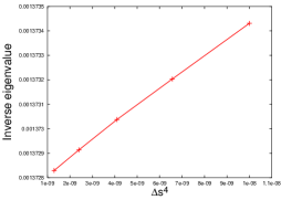
Figure 8: First inverse eigenvalue of the response function ${\bf S}$ a lamellar phase vs. $\Delta{s}^{4}$ when the perturbation theory is evaluated using the extrapolation scheme of Eq. 58.

Appendix B Body- and Face-Centered Lattices

Here, we explain an issue that we encountered when calculating band diagrams for BCC and Gyroid phases using a non-primitive cubic unit cell. Analogous issues can arise whenever a body- or face-centered crystal is treated with a non-primitive computational unit cell.

Band diagrams for the BCC and Gyroid phases, can be calculated using either a cubic unit cell with orthogonal axes, or a primitive unit cell with non-orthogonal axes, which has half the volume of the cubic unit cell. (The Gyroid structure is based on a BCC lattice). We have used a simple cubic computational unit cell with cell size $a$, and discretized this with a simple cubic FFT grid. The reciprocal lattice associated with this computational unit cell thus includes wavevectors that are not part of the reciprocal lattice of the BCC Bravais lattice, which is an FCC lattice in $k$-space. The first Brillouin zone (FBZ) associated with the simple cubic unit cell ($|k_{x}|,|k_{y}|,|k_{z}|<\pi/2$) has half the volume in $k$-space as the FBZ for the BCC unit cell.

If the algorithm described in this paper is applied to a BCC structure using a simple cubic cell, without explicitly accounting for the centering symmetry of the unperturbed structure, the list of eigenvalues obtained at a specified ${\bf k}$ in the FBZ of the simple cubic cell include both those associated with ${\bf k}$ and those associated with another wavevector ${\bf k}^{\prime}={\bf k}+{\bf G}$ that differs from ${\bf k}$ by a lattice vector ${\bf G}=(\pm 1,0,0)2\pi/a$, $(0,\pm 1,0)2\pi/a$, or $(0,0,\pm 1)2\pi/a$ that is part of the simple cubic reciprocal lattice, but not part of the reciprocal lattice of BCC. The vectors ${\bf k}$ and ${\bf k}^{\prime}$ are thus equivalent from the point of view of the simple cubic lattice but inequivalent from the point of view of the BCC lattice. Correspondingly, if ${\bf k}$ lies in the FBZ of the simple cubic cell, then ${\bf k}^{\prime}$ generally lies within the FBZ of the BCC unit cell but the outside the smaller FBZ of the simple cubic unit cell. The result is a “folding” of the FBZ of the BCC unit cell into the smaller FBZ of the simple cubic computational unit cell.

The problem could be avoided either by using a primitive BCC unit cell from the outset, or by using only the reciprocal vectors of the BCC unit cell in the calculation of $S_{ij}({\bf G},{\bf G}^{\prime};{\bf k})$. What we have actually done is to use our machinery for generating symmetrized basis functions to generate basis functions that are invariant under a subgroup of $L({\bf k})$ group that, at a minimum, includes the identity ${\bf r}\rightarrow{\bf r}$ and the body-centering translational symmetry ${\bf r}\rightarrow{\bf r}+(1,1,1)a/2$. This guarantees that we will only obtain eigenfunctions of the Bloch form $e^{i{\bf k}\cdot{\bf r}}\psi_{n}({\bf r})$ in which $\psi_{n}({\bf r})$ has the periodicity of the BCC lattice, and not just the periodicity of the larger cubic cell. If only these two symmetry elements are included, the algorithm automatically generates basis functions that are simply plane waves with wavevectors that belong to the reciprocal lattice for BCC, while discarding the remaining “extinct” reciprocal lattice vectors of the simple cubic lattice. The advantage of this approach is its generality: It allows the use of either primitive or non-primitive unit cells, generalizes immediately to the treatment of other kinds of body- and face-centered crystals, and does not require the explicit addition of special extinction conditions to our algorithm.

References

- de Gennes 1979 P.-G. de Gennes, Scaling Concepts in Polymer Physics (Cornell University Press, 1979).
- Nozieres and Pines 1958a P. Nozieres and D. Pines, Physical Review 109, 741 (1958a).
- Nozieres and Pines 1958b P. Nozieres and D. Pines, Physical Review 109, 762 (1958b).
- Pines and Nozieres 1989 D. Pines and P. Nozieres, Theory of Quantum Liquids (Addison Wesley Publishing Company, 1989).
- Ashcroft and Mermin 1976 N. W. Ashcroft and N. D. Mermin, Solid State Physics (Saunders College Publishers, 1976).
- Ziman 1972 J. M. Ziman, Principles of the Theory of Solids (Cambridge University Press, 1972).
- Leibler 1980 L. Leibler, Macromolecules 13, 1602 (1980).
- Shi et al. 1996 A.-C. Shi, J. Noolandi, , and R. C. Desai, Macromolecules 29, 6487 (1996).
- Laradji et al. 1997a M. Laradji, A.-C. Shi, R. C. Desai, and J. Noolandi, Physical Review Letters 78, 2577 (1997a).
- Laradji et al. 1997b M. Laradji, A.-C. Shi, R. C. Desai, and J. Noolandi, Macromolecules 30, 3242 (1997b).
- Matsen and Schick 1994 M. W. Matsen and M. Schick, Physical Review Letters 72, 2660 (1994).
- Matsen 1998a M. W. Matsen, Physical Review Letters 80, 440 (1998a).
- Matsen 2001 M. W. Matsen, Journal of Chemical Physics 114, 8165 (2001).
- Rasmussen and Kalosakas 2002 K. O. Rasmussen and G. Kalosakas, Journal of Polymer Sci. B 40, 1777 (2002).
- Sides and Fredrickson 2003 S. W. Sides and G. H. Fredrickson, Polymer 44, 5859 (2003).
- Cochran et al. 2006 E. W. Cochran, C. J. Garcia-Cervera, and G. H. Fredrickson, Macromolecules 39, 2449 (2006).
- Fredrickson 2006 G. H. Fredrickson, The Equilibrium Theory of Inhomogeneous Polymers (Clarendon Press, Oxford, 2006).
- Shi 1999 A.-C. Shi, J. Phys: Condensed Matter 11, 10183 (1999).
- Bouckaert et al. 1936 L. P. Bouckaert, R. Smoluchowski, and E. Wigner, Physical Review 50, 58 (1936).
- Tinkham 1964 M. Tinkham, Group Theory and Quantum Mechanics (McGraw-Hill Book Company, 1964).
- Sakurai et al. 1993 S. Sakurai, H. Kawada, T. Hashimoto, and L. J. Fetters, Macromolecules 26, 5796 (1993).
- Jones 1975 H. Jones, Theory of Brillouin zones and Electronic States in Crystals (North Holland Publishing Company, Amsterdam, 1975).
- Tyler and Morse 2005 C. A. Tyler and D. C. Morse, Physical Review Letters 94, 208302 (2005).
- Tyler et al. 2007 C. A. Tyler, J. Qin, F. Bates, and D. C. Morse, Macromolecules 40, 4654 (2007).
- Ranjan and Morse 2006 A. Ranjan and D. C. Morse, Physical Review E 74, 011803 (2006).
- Matsen 1998b M. W. Matsen, Physical Review Letters 80, 201 (1998b).
- Deuflhard and Mornemann 2002 P. Deuflhard and G. Mornemann, Scientific Computing with Ordinary Differential Equations (Springer-Verlag New York Inc., 2002).