Nuclear Bar Catalyzed Star Formation: ¹³CO, C¹⁸O and Molecular Gas Properties in the Nucleus of Maffei 2

Abstract

We present $\sim 3^{{}^{\prime\prime}}$ resolution maps of CO, its isotopologues, and HCN from in the center of Maffei 2. The J=1–0 rotational lines of ¹²CO, ¹³CO, C¹⁸O and HCN, and the J=2–1 lines of ¹³CO and C¹⁸O were observed with the OVRO and BIMA arrays. The lower opacity CO isotopologues give more reliable constraints on H₂ column densities and physical conditions than optically thick ¹²CO. The J=2–1/1–0 line ratios of the isotopologues constrain the bulk of the molecular gas to originate in low excitation, subthermal gas. From LVG modeling, we infer that the central GMCs have $n_{H_{2}}\sim 10^{2.75}~{}cm^{-3}$ and T${}_{k}~{}\sim 30$ K. Continuum emission at 3.4 mm, 2.7 mm and 1.4 mm was mapped to determine the distribution and amount of H II regions and dust. Column densities derived from C¹⁸O and 1.4 mm dust continuum fluxes indicate the standard Galactic conversion factor overestimates the amount of molecular gas in the center of Maffei 2 by factors of $\sim$2-4. Gas morphology and the clear “parallelogram” in the Position-Velocity diagram shows that molecular gas orbits within the potential of a nuclear ($\sim$220 pc) bar. The nuclear bar is distinct from the bar that governs the large scale morphology of Maffei 2. Giant molecular clouds in the nucleus are nonspherical and have large linewidths, due to tidal effects. Dense gas and star formation are concentrated at the sites of the $x_{1}-x_{2}$ orbit intersections of the nuclear bar, suggesting that the starburst is dynamically triggered.

1 Introduction

Concentrations of molecular gas are common in the centers of large spiral galaxies, often in the form of nuclear bars. Bars represent likely mechanisms by which rapid angular momentum loss and gas inflow concentrate gas in the centers of galaxies (eg. Sakamoto et al., 1999; Sheth et al., 2005; Knapen, 2005). Secondary nuclear bars can be important in controlling the dynamics of the innermost few hundred parsecs of galaxies (eg., Shlosman, Frank & Begelman, 1989; Friedli & Martinet, 1993; Heller et al., 2001; Maciejewski et al., 2002; Shlosman & Heller, 2002; Englmaier & Shlosman, 2004). In addition to being an avenue by which nuclear gas and stellar masses are built up, these bars can also significantly influence the physical and chemical properties of molecular clouds within them (eg. Meier & Turner, 2001; Petitpas & Wilson, 2003; Meier & Turner, 2004, 2005).

We have observed the two lowest rotational lines of ¹³CO and C¹⁸O, plus new high resolution images of ¹²CO(1-0) and HCN(1-0) in the nearby galaxy, Maffei 2, with the Owens Valley Millimeter (OVRO) Array and the Berkeley-Illinois-Maryland Association Array (BIMA). Because they are optically thin, or nearly so, CO isotopologues more directly trace the entire molecular column density than does optically thick ¹²C¹⁶O (hereafter “CO”). Also ratios amongst isotopologues are more sensitive to changes in density and temperature throughout the clouds. HCN, which has a higher critical density than CO, constrains the dense molecular cloud component. Here we aim to characterize the properties of molecular clouds in the center of this barred galaxy, and to connect those properties with the dynamics of the nucleus.

Maffei 2 is one of the closest large spirals (D$\simeq$3.3 Mpc, $\S$2; Table Nuclear Bar Catalyzed Star Formation: ¹³CO, C¹⁸O and Molecular Gas Properties in the Nucleus of Maffei 2), but lies hidden behind more than 5 magnitudes of Galactic visual extinction (Maffei, 1968). A disturbed, strongly barred spiral galaxy (Hurt et al., 1993a; Buta & McCall, 1999), Maffei 2 has an asymmetric HI disk and tidal arms that suggest a recent interaction with a small satellite (Hurt, Turner & Ho, 1996). The interaction may be responsible for the bright nuclear CO emission (eg., Rickard, Turner & Palmer, 1977; Ishiguro et al., 1989; Mason & Wilson, 2004) and active nuclear star formation of L${}_{OB}~{}\simeq~{}1.7\times 10^{9}~{}$L_⊙ (Turner & Ho, 1994, corrected for distance).

2 Distance to Maffei 2

Galactic extinction complicates distance determinations for this nearby ($V_{LSR}$=-30 km s^-1) galaxy. Some have suggested that Maffei 2 is close enough to have a significant dynamical influence on the Local Group (Buta & McCall, 1983; Zheng, Valtonen & Byrd, 1991). Estimated distances to the members of the IC 342/Maffei 2 group range from 1.7–5.3 Mpc (Buta & McCall, 1983; McCall, 1989; Luppino & Tonry, 1993; Karachentsev & Tikhonov, 1993, 1994; Krismer, Tully & Gioia, 1995; Karachentsev et al., 1997; Ivanov et al., 1999; Davidge & van den Bergh, 2001). Closer distances (D${}_{mpc}~{}\sim$ 2) tend to come from the Faber-Jackson relationship and the brightest supergiants method (Buta & McCall, 1983; Karachentsev & Tikhonov, 1993, 1994; Karachentsev et al., 1997), while the farther distances (D${}_{mpc}~{}\sim$ 4–5) come from Tully-Fisher relations on Maffei 2 and surface brightness fluctuations methods towards its companion Maffei 1 (Hurt, 1993; Luppino & Tonry, 1993; Krismer, Tully & Gioia, 1995; Ivanov et al., 1999). In several cases, the same method gives wide ranges of distances for different galaxies within the same group, suggesting the group is spatially extended (likely) or each distance measurement has higher uncertainties than claimed (Krismer, Tully & Gioia, 1995; Karachentsev et al., 1997). Recent studies appear to be converging to D $\sim$ 3-3.5 Mpc for the IC 342/Maffei 2 group (Saha, Claver, & Hoessel, 2002; Fingerhut et al., 2003; Karachentsev et al., 2003; Karachentsev, 2005; Fingerhut et al., 2007). Fingerhut et al. (2007) do a self consistent analysis of several different measurements and obtain a distance of 3.3 Mpc. We adopt this distance for Maffei 2, with uncertainties of $\sim$ 50 %. Quoted uncertainties in this paper do not include this systematic uncertainty.

3 Observations

Aperture synthesis observations of the ¹³CO(1-0), ¹³CO(2-1), C¹⁸O(1-0), C¹⁸O(2-1) and HCN(1-0) lines were obtained with the Owens Valley Radio Observatory (OVRO) Millimeter Array between 1993 October 26 and 1999 March 29. The ¹³CO(1-0) and ¹³CO(2-1) data were obtained when the OVRO array had five 10.4 meter antennas, while the remaining data are from the six-element array (Padin et al., 1991; Scoville et al., 1994). Observing parameters are listed in Table 2. Separate 1 GHz bandwidth continuum channels at 3.4 mm, 2.7 mm and 1.4 mm were also recorded. 3C84 and 0224+671 were used to calibrate instrumental amplitudes and phases. Absolute fluxes were calibrated using Neptune, Uranus and 3C273 as standards, with additional observations of 3C84 and 3C454.3 as consistency checks. Absolute flux calibration should be good to 10 – 15% for the 3 mm data and 20 – 25% for the 1 mm data, and internally consistent between each transition.

We have also obtained high resolution ($\sim 3^{{}^{\prime\prime}}$) observations of the ¹²CO(1-0) transition with the ten element Berkeley-Illinois-Maryland Association (BIMA) Array (Welch et al., 1996). Phase calibration was done with 0224+671 and the ultracompact H II region W3(OH) was used for flux calibration.

Each OVRO track includes at least two phase centers separated by less than the FWHM power points of the primary beams of the dishes (Table 2). The pointings were naturally weighted and mosaiced using the MIRIAD. Quoted noise levels are the rms from line-free channels of the spectral cube half-way between the map centers and edges. The true noise level is slightly lower ($\sim 10\%$) at the phase centers and somewhat higher towards the edge of the primary beams due to the mosaicing. Subsequent data analysis was done with the NRAO AIPS.

Since interferometers act as spatial filters, it is important that emission maps being compared have similar $(u,v)$ coverage, including minimum baselines. For the 3 mm lines observed with OVRO, the $(u,v)$ coverage is very similar. For the J=2–1 lines at $\lambda=1$ mm, the $(u,v)$ coverage is consistent (C¹⁸O(1–0) and C¹⁸O(2–1) were observed simultaneously), but scaled up by a factor of two from their 3 mm counterparts ( $(u,v)=B_{proj}/\lambda$, projected baselines in the east-west and north-south directions respectively). The 2–1 transitions were tapered to match the $(u,v)$ range of the corresponding 1–0 transition. For the OVRO datasets, the minimum (1–0) [(2–1)] baselines are $(u,v)_{min}\simeq 5.5~{}k\lambda$ [$11~{}k\lambda$]. Thus the images are insensitive to emission on spatial scales $\mbox{$\stackrel{{\scriptstyle>}}{{{}_{\sim}}}$}35$–$40^{{}^{\prime\prime}}$ ($\sim$500–600 pc) for 110 GHz and $\mbox{$\stackrel{{\scriptstyle>}}{{{}_{\sim}}}$}20^{{}^{\prime\prime}}$ ($\sim$300 pc) for 220 GHz. For the ¹²CO(1–0) transition, observed at BIMA, uv coverage is similar to the OVRO 3 mm uv coverage ($(u,v)_{min}~{}\sim 5.4~{}k\lambda$).

We have estimated the amount of flux resolved out of each map due to missing short spacings. Single-dish spectra of ¹²CO(1–0), ¹³CO(1–0), ¹³CO(2–1) and HCN(1–0) exist for Maffei 2 in the literature (Table 2.) The interferometer map for each line was convolved to the beamsize of the single-dish and then sampled at the same pointing center. Within uncertainties, all of the flux of the CO(1–0) and ¹³CO(1–0) lines is detected. The ¹³CO(2–1) and HCN(1–0) maps recover $\sim$ 60% of the single dish flux, although the single-dish ¹³CO(2–1) flux measurement is rather uncertain (Wild et al., 1992). We expect the interferometer to recover fractions of C¹⁸O flux similar to the corresponding ¹³CO lines.

To generate integrated intensity maps, a mask was made by convolving the channel maps to 10${}^{{}^{\prime\prime}}$ resolution, then blanking regions of emission $<$ 2$\sigma$. This mask was then used to blank out non-signal portions for the full resolution channel cube. Velocities from -160 km s^-1 to 100 km s^-1 were integrated, including emission $>$1.2$\sigma$ in the full resolution channel maps. For the line ratio maps, the integrated intensity maps were convolved with an elliptical Gaussian to the beam size of the lowest resolution maps (¹³CO(1–0) and C¹⁸O(1–0)). This gives a resolution of $\sim 3.9^{{}^{\prime\prime}}$ for the line ratio maps. Regions of emission $<$ 3$\sigma$ in either line (2$\sigma$ for the C¹⁸O(2–1)/C¹⁸O(1–0) map) were blanked in making the ratio maps. Because of the uncertainties in fluxes and absolute positions, the ratio maps are estimated to be accurate to $\sim$ 35–40% in magnitude, and $\sim 2^{{}^{\prime\prime}}$ in position (excluding possible systematic errors associated with differences in resolved-out flux).

Since Maffei 2 is within 1° of the Galactic Plane, and at essentially zero redshift, we have to consider the possibility of contamination from Galactic CO. Galactic HI emission significantly affects VLA images of Maffei 2 in the velocity range -70 km s^-1–0 km s^-1 (Hurt, Turner & Ho, 1996), with the strongest absorption at -40 km s^-1. Galactic HI emission is more widespread than CO emission, however, and what CO emission there is near Maffei 2 has very narrow lines ($<$ few km s^-1, based on our spectra from the late NRAO 12 Meter Telescope.) Inspection of our channel maps reveals no obvious evidence of Galactic CO emission, and so we disregard it.

4 Molecular Gas in the Center of Maffei 2: Overview

4.1 Gas Morphology

CO emission in Maffei 2 takes the form of two prominent and highly inclined arms (Ishiguro et al., 1989), which form the molecular bar, as shown in the integrated intensity maps of Figure 1. The emission extends roughly 1$\farcm$5 (1440 kpc) along the major axis (Table 3). The brightest CO emission emerges from clouds within the central 15″ ($\sim$240 pc) of the galaxy.

A higher (2″; $\sim$30 pc) resolution, uniformly-weighted image of CO(1–0) (Figure 2a) shows that the bright CO peaks resolve into GMCs. The central two CO peaks become a nuclear ring of radius $\sim$5″, or $\sim$80 pc about the dynamical center. The eastern side of this ring is brighter in CO(1–0) but ¹³CO(1–0) remains rather uniform. The molecular arms are roughly linear features running northeast and southwest, terminating at the central ring. Peak observed brightness temperatures, T${}_{mb},$ reach $\simeq$ 31 K, and are typically $\stackrel{{\scriptstyle>}}{{{}_{\sim}}}$ 10 K across much of the arms.

Cloud properties—size, linewidth, temperature, mass—are derived for the brightest molecular clouds in Maffei 2, using the uniformly-weighted CO(1–0) image (Figure 2c). Following Meier & Turner (2001, 2004) (Table 4), a molecular cloud is defined as a region of spatially and spectrally localized emission greater than 2$\sigma$ in two adjacent channels, but need not necessarily be a gravitationally bound entity. Each cloud was fit from channel maps that include only the gas over its localized velocity range. Clumps separated by one beamwidth or less are considered the same GMC. Cloud complexes are labeled A–H based on their locations in the lower resolution maps; sub-clumps resolved in the higher resolution image are numbered.

Most of the GMCs are resolved along at least one axis, with sizes of $\sim$40–110 pc (Table 4). The clouds are significantly elongated, with axial ratios often greater than 2. Typical position angles of the clouds, 20-60°, are very similar to the sky plane position angle of the bar, $\sim$40°. This is not an artifact of the beam shape, since the beam is elongated perpendicular to the bar. Nor is the elongation due to an underlying smooth gas component along the bar, since fits come only from maps localized in velocity. If the elongation of the clouds is a foreshortening effect due to the high inclination of Maffei 2 (67°; Table Nuclear Bar Catalyzed Star Formation: ¹³CO, C¹⁸O and Molecular Gas Properties in the Nucleus of Maffei 2), then the GMCs must be flattened perpendicular to the plane of the galaxy, that is, disk-like, rather than spherical. However, since similar elongations are observed in the molecular clouds along the bar in the nucleus of the face-on galaxy IC 342 (Meier & Turner, 2001), we consider cloud elongation along the bar more likely. The shapes of the nuclear GMCs are clearly affected by their location within the bar.

With the exception of two small GMCs (D2 and H1), cloud linewidths are $>50$ km s^-1 FWHM, and approach $\sim$ 100 km s^-1 in a couple of locations. If these clouds were in virial equilibrium, then their individual masses would be in excess of $10^{7}M_{\odot}$. However, these clouds are very unlikely to be in virial equilibrium (§6). This is further demonstrated by the fact that there is no correlation between the size $(\sqrt{ab})$ and $\Delta v_{1/2}$ in Table 4.

The CO isotopologues generally follow the brighter CO emission, but there are subtle differences. Weak ¹³CO(1-0) emission (Fig. 1b) extends to the map’s edge, roughly along the major axis of the large-scale near-infrared (NIR) (Hurt et al., 1993a) and the large-scale molecular bar (Mason & Wilson, 2004). The ¹³CO(2-1) emission (Fig. 1e) is found mostly at cloud peaks due to the higher critical density ($A_{ij}$) of the J=2–1 line, but some diffuse gas not associated with the clumps is resolved out. Little emission off the trailing southwestern CO arm ridges (GMC H) is seen in ¹³CO.

C¹⁸O emission (Figs. 1c and 1f) follows ¹³CO, but the C¹⁸O linewidths are slightly narrower. This may be a critical density effect, with the lower opacity C¹⁸O more confined to the dense cores. As a result of these spatial differences, comparisons of C¹⁸O line intensities with ¹²CO and ¹³CO will slightly overestimate their true temperature ratios. Peak main-beam temperatures are T${}_{mb}\simeq 0.5$ K (T${}_{mb}\simeq 1.0$ K) in a $3\farcs 9\times 3\farcs 4$ beam ($2\farcs 4\times 2\farcs 3$) for C¹⁸O(1-0) (C¹⁸O(2-1)).

The HCN(1–0) map is shown in Figure 1d. Because of its much larger electric dipole moment ($\sim$30 times CO), HCN has a critical density nearly 1000 times higher than CO, and traces high density gas. HCN predominately traces the two inner peaks of GMCs D+E and F. HCN(1–0) emission falls off with distance from the center of the galaxy faster than seen in any of the other lines (note particularly GMC G). There is also evidence that the HCN is more strongly confined to the GMCs than CO or ¹³CO. Apparently the densest molecular gas is localized more strongly to the very center of the galaxy.

4.2 Star Formation in Maffei 2: Millimeter Continuum Images of H II Regions and Dust

Continuum maps of Maffei 2 at 3.4 mm, 2.7 mm and 1.4 mm are presented in Figure 3, along with the 2 cm VLA maps from Turner & Ho (1994). The 3.4 mm continuum has been corrected for the contribution of HCN and HCO⁺ lines within the bandpass, and the 2.7 mm continuum map for the contribution of ¹³CO. The advantage of imaging continuum at 3 mm is that this is the part of the spectrum where the free-free emission component from H II regions is at its maximum relative to other sources of emission, such as nonthermal synchrotron and thermal dust emission.

There are three main 3.4 mm continuum sources near the center of Maffei 2, with weaker sources towards the southwestern bar end (GMC G) (Table 5). Four central sources are found at 2 cm; source III has a non-thermal spectral index between 6 cm and 2 cm (Turner & Ho, 1994), and is predictably absent in the millimeter maps. Sources I & II are coincident with GMCs D and E and each have fluxes of $\sim$ 5.8 mJy. Source IV is just north of GMC F and has a flux of $\sim$ 5.0 mJy. The non-thermal source III is not associated with any of the bright GMCs. At higher resolution these continuum sources resolve into a collection of SNR and H II regions (Figure 2d; Tsai et al., 2006).

Spectral energy distributions (SEDs) for each of the main radio sources are shown in Figure 4. Three components are fit: synchrotron, bremsstrahlung (free-free) and dust, with spectral indices of -0.7, -0.1 and 3.5 ($\beta=1.5$) respectively:

$$S_{source}=S^{4.9}_{syn}\left(\frac{\nu}{4.885}\right)^{-0.7}+S^{89}_{ff}\left(\frac{\nu}{88.92}\right)^{-0.1}+S^{219}_{d}\left(\frac{\nu}{219.3}\right)^{3.5}.$$

Estimated fluxes for free-free and dust emission are recorded in Table 6. At cm wavelengths, the central continuum sources have spectral indices between 6 cm and 2 cm, $\alpha^{6}_{2}$, of -0.63 ($S_{\nu}\propto\nu^{\alpha}$), and therefore are dominated by synchrotron emission. The spectral index between 2 cm and 3.4 mm, $\alpha^{2}_{3.4}$, flattens to -0.1 – -0.3, as expected for H II regions dominated by free-free emission. There can be mixtures of synchrotron and free-free emission within our beam; we have also shown cm-wave fluxes for the compact sources (Tsai et al., 2006, corrected for distance) for comparison in Figure 4. Our fits indicate that towards I, II and IV the 3 mm continuum emission is dominated by the compact, free-free emission sources.

The 1.4 mm continuum map is shown in Figure 3d, convolved to the resolution of the 2.7 mm map. Emission peaks towards Source II at $\sim$21 mJy beam^-1. Continuum fluxes at 1.4 mm are larger than the 3.4 or 2.7 mm fluxes, indicating a rising spectral index between 2.7 mm and 1.4 mm, $\alpha_{2.7}^{1.4}$, of +1.5. The 1.4 mm emission is therefore a mixture of free-free and dust emission, with the predominance of dust varying with position. The total flux associated with dust emission, after removing the estimated thermal free-free contribution, is $S_{1.4mm}\sim$7–19 mJy for each source.

5 Gas Excitation and Opacity Across the Nucleus of Maffei 2

Excitation temperatures are important for understanding molecular gas properties and how they vary across the nucleus. The J=2–1 and J=1–0 lines are sensitive to relatively cool gas in GMCs, and the low J CO lines, especially CO(1–0), are thermalized in all but the lowest density molecular clouds. CO isotopologues thermalize at somewhat higher densities ($\mbox{$\stackrel{{\scriptstyle>}}{{{}_{\sim}}}$}10^{3}$ cm^-3) due to their lower opacity, making them excellent probes of gas excitation in this density regime.

5.1 Excitation Temperatures

Excitation temperatures, T_ex, are constrained by the ratios of integrated intensities of the J = 2–1 and J = 1–0 lines,

$${\int^{i}T_{21}dv\over\int^{i}T_{10}dv}\simeq{{}^{i}f_{21}(^{i}J_{21}(T_{ex})-^{i}J_{21}(T_{cmb}))(1-e^{-^{i}\tau_{21}})\over{}^{i}f_{10}(^{i}J_{10}(T_{ex})-^{i}J_{10}(T_{cmb}))(1-e^{-^{i}\tau_{10}})},$$ (1)

where ${}^{i}J_{\nu}(T_{ex})~{}=~{}(h\nu/k)/(exp\{h\nu/kT_{ex}\}-1)$, ${}^{i}\tau_{ul}$ and ${}^{i}f_{ul}$ are the optical depth and filling factors of the $i$th isotopologue, respectively. We assume LTE (constant T_ex with J) throughout the cloud. Limitations of this assumption are noted below.

The ¹³CO(2–1)/¹³CO(1–0) line ratios for the nuclear bar are shown in Figure 5 (Table 7). Values range from 0.3 to 0.8, corresponding to T${}_{ex}\simeq 3$–6 K if ¹³CO is optically thin, or up to 10 K, if completely thick. This ratio peaks towards the central two GMC complexes (GMC D+E & F), and falls with increasing radial distance. C¹⁸O(2–1)/C¹⁸O(1–0) is also higher at the central two emission peaks, with values of $\sim$ 0.68–0.79. C¹⁸O is almost certainly optically thin. From C¹⁸O(2–1)/C¹⁸O(1–0), we obtain T${}_{ex}\sim$5.4–6 K (Table 8). There are several regions off the GMCs (between C and D; H2) that have higher ratios. The ratios are largest between clouds: perhaps the intercloud gas is warmer than the GMCs (although emission is weak here). Figure 6 shows the average peak T_mb ratios schematically as a function of velocity to show changes in excitation along the central ring. The eastern side of the central ring has the highest T_ex and this is the side closest to the starburst.

T_ex based on the isotopologues are significantly lower than both the T_ex implied by the single dish CO(2-1)/CO(1-0) line ratio of $\mbox{$\stackrel{{\scriptstyle>}}{{{}_{\sim}}}$}2$ (Sargent et al., 1985) and the brightness temperatures, T_mb, estimated from the high resolution CO(1–0). Single-dish CO(3-2)/CO(1-0) line ratios are also high, $\sim$1.3–1.8 (Hurt et al., 1993b; Dumke et al., 2001), as are ¹³CO(3-2)/¹³CO(2-1) ratios (1.6; Wall et al., 1993). These CO ratios suggest that there is warm, optically thin gas with T${}_{k}\mbox{$\stackrel{{\scriptstyle>}}{{{}_{\sim}}}$}50$ K. Other molecules indicate a range of gas temperatures. From ammonia, Takano et al. (2000) find a rotational temperature of $T_{rot}\sim$30 K that is constant across the field, and an ortho-to-para ratio consistent with formation at 13 K. Henkel et al. (2000) obtain $T_{rot}$= 85 K, based predominantly on the inclusion of the the high energy metastable transition, (J,K) = (4,4). However, they point out that it is possible to fit the four lowest metastable transitions with a cool component and a warm component. Rieu et al. (1991) derived a low T_ex of 10 K from a multi-line study of HNCO.

Excitation of molecular clouds in the nucleus of Maffei 2 is complex, and different molecular transitions will find different values for T_ex, depending on where the molecules are found. Some of the differences in line ratios between CO, its optically thinner isotopologues, and other molecular tracers, are due to the isotopologues being subthermally excited relative to CO, such that T_ex $<$ T_k because $n_{H_{2}}~{}<~{}n_{crit}(CO)$. If the densities determined from the LVG analysis are correct then the T_ex of the isotopologues imply kinetic temperatures of T_k = 15 - 35 K (§7). These are close to but still slightly cooler than the (cool component of) ammonia. Thus the bulk of molecular gas, traced by the optically thinner species, is cool. However CO emission is unlikely to be subthermal at these densities. So the high single-dish CO line ratios are inconsistent with the physical conditions of this component and require the presence of some warmer gas. Whether the emission from the high opacity CO transitions originates in warmer envelopes of the clouds (as in IC 342, Turner et al., 1993; Meier & Turner, 2001), or from a compact, dense component (possibly associated with the high temperature ammonia component) remains unclear from the current data. The low T_ex of the higher critical density HNCO may argue against the latter, but spatially-dependent chemical effects may also be involved here.

5.2 Opacity of the ¹³CO and C¹⁸O Lines

The opacity of the ¹³CO line is important for mass determinations and the interpretation of brightness temperatures. Based on the large CO(3–2)/¹³CO(1–0) ratio, Hurt et al. (1993b) estimated that the $\tau_{13CO(1-0)}\sim 0.1$, or that $\tau_{CO(1-0)}$ is only 5–7, on the assumption that CO(3–2) and ¹³CO(1–0) have the same T_ex. With higher spatial resolution this now appears not to be the case.

Better opacity estimates are obtained by avoiding ratios taken between lines with widely different opacities, particularly in situations where temperature gradients and other non-LTE effects may be present. The ¹³CO(1-0)/¹⁸CO(1-0) integrated intensity ratio map of Maffei 2 is shown in Figure 5f. Values range from 2.4–4.3. The line ratio is lower than expected if the ¹³CO(1-0) line (and the ¹⁸CO(1-0) line) have negligible opacities for adopted abundance ratios of [H₂]/[¹³CO]=$4.7\times 10^{5}$ and [H₂]/[C¹⁸O]=$2.9\times 10^{6}$, or [¹²CO]/[H₂] = $8.5\times 10^{-5}$, [¹²CO]/[¹³CO] = 60 and [C¹⁶O]/[C¹⁸O]=250 (Frerking et al., 1982; Henkel et al., 1994; Wilson & Rood, 1994; Wilson, 1999; Milam et al., 2005). These isotopic abundances are typical of what is measured in nearby starbursts (eg. Henkel et al., 1994), and are within a factor of $\sim$2 of the entire range observed in the Galaxy. A ¹³CO(1–0)/¹⁸CO(1–0) line ratio of 3.0 implies $\tau_{13CO(1-0)}\simeq 1$, for these isotopic abundance ratios.

Uncertainties in derived opacities depend sensitively on the true [¹³CO/C¹⁸O] abundance ratio which may differ from the value adopted here. Both [CO/¹³CO] and the [CO/C¹⁸O] decrease with stellar processing (assuming the CO isotopologues abundances are proportional to their respective isotopic abundances). Based on Galactic disk studies, [¹³CO/C¹⁸O] is expected to decrease from $\sim$7.5 in the local ISM to $\sim$4 in the inner kpc of the disk, arguing for a decrease in the combined ratio with nuclear synthesis (eg. Wilson, 1999; Milam et al., 2005). Attempts to determine isotopic abundances directly in starbursts obtain ¹³CO/C¹⁸O $\simeq$ 5, further supporting a lower ratio in high metallicity regimes (eg. Henkel et al., 1994). On the other hand, Galactic Center (Sgr B2) determinations arrive at anomalously high values of [¹³CO/C¹⁸O] $\sim$10 (eg. Langer & Penzias, 1990). Using the Galaxy as a guide [¹³CO/C¹⁸O] should fall somewhere between 4 and 10. We favor values on the low end of this range for the high metallicity nucleus of Maffei 2 for three reasons: (1) The Galactic disk gradient and the starburst values imply low ratios in heavily processed locations. (2) The LVG models give consistent ¹³CO and C¹⁸O parameter space solutions for value [¹³CO/C¹⁸O] $\simeq$ 4, but not for 10 (§7). (3) There is marginally significant evidence for lower CO(1–0)/¹⁸CO(1–0) and ¹³CO(1–0)/¹⁸CO(1–0) line ratios along the central ring, even towards the lower column density portions (Figure 6). This may represent direct evidence for enrichment of C¹⁸O relative to ¹³CO (and CO) in the immediate vicinity of the nuclear starburst (similar effects are seen in IC 342; Meier & Turner, 2001).

Modulo small differences in resolved-out flux or linewidth, we conclude $\tau_{13CO(1-0)}\sim 1$ over the molecular peaks, but note that systematic abundance uncertainties allow anything between $\tau\ll$ 1 up to $\tau\sim$ 4. The fact that the CO(3–2)/¹³CO(1–0) line ratios of Hurt et al. (1993b) imply much lower opacities must then be a result of CO(3–2) emission (and likely CO in general) preferentially originating from higher excitation gas than do ¹³CO(1–0) and ¹⁸CO(1–0).

With $\tau_{13CO(1-0)}$ independently constrained from the ¹³CO/C¹⁸O ratio, comparisons between T_ex derived from eq. (1) (corrected for resolved out flux) and the observed ¹³CO(1–0) peak brightness temperature, ¹³T_mb, gives constraints on the filling factor, ${}^{13}f$, via ${}^{13}f~{}\sim$ [¹³T${}_{mb}/^{13}J_{10}(T_{ex})](1-e^{-\tau_{13CO(1-0)}})^{-1}$. Towards the molecular peaks ${}^{13}f$ $\sim$ 0.33 is estimated. Given the potentially large uncertainty in the estimate of the average ¹³CO opacity, ${}^{13}f$ should be considered only indicative. If $\tau_{13CO(1-0)}\gg$ 1 then ${}^{13}f$ could be as low as $\sim$0.15. The relatively bright ¹³CO(1–0) emission and the fact that ${}^{13}f~{}\leq$ 1 requires that $\tau_{13CO(1-0)}\mbox{$\stackrel{{\scriptstyle>}}{{{}_{\sim}}}$}$ 0.33.

In summary, the J= 2–1 to 1–0 line ratios of the lower opacity CO isotopomers imply LTE excitation temperatures of T${}_{ex}\sim$3-10 K. Brightnesses of the higher opacity J $>$ 1 transitions of CO, suggest that they preferentially sample more limited volumes of warmer gas. The opacity of the ¹³CO(1–0) transition appears to approaches unity over much of the nuclear peaks.

5.3 HCN

We also compare the distribution of dense gas traced by HCN to that of the total gas traced by CO. Figure 5c, shows the CO(1–0)/HCN(1–0) integrated intensity line ratio. The ratio varies from $\sim$8 at GMC F to $>$20 at the ends of the molecular bar. Figure 5c shows the general radial trend commonly seen in galaxies, namely an increase in the CO/HCN intensity ratio as one moves away from the star forming sites at the center (e.g., Helfer & Blitz, 1993, 1997; Sorai et al., 2002). Sites of high CO(1–0)/¹³CO(1–0) ratios (particularly in the off-arm regions) also have the highest CO(1–0)/HCN(1–0) ratios (Table 7). This provides evidence that the ¹³CO(1–0) is at least partially sensitive to the density of the gas.

6 Nuclear Gas Kinematics: The Parallelogram and a Bar Model

Maffei 2 is a strongly barred galaxy with a disturbed morphology, probably due to interaction with a nearby companion (Hurt et al., 1993a; Hurt, Turner & Ho, 1996; Mason & Wilson, 2004). Position-Velocity (P-V) diagrams based on lower resolution CO(1-0) data, show that the molecular gas in the central regions reaches high ($\stackrel{{\scriptstyle>}}{{{}_{\sim}}}$ 75 km s^-1) radial velocities over very small projected radii (Ishiguro et al., 1989; Hurt & Turner, 1991). Ishiguro et al. (1989) has interpreted this feature as an expanding ring generated by an explosive event some $\sim 5\times 10^{6}$ yrs ago, superimposed on a Keplerian component. Since Maffei 2 is strongly barred, it is reasonable to consider whether these motions are a result of non-circular motions due to a barred potential. Ishiguro et al. (1989) argued against this based on the fact the position angle of the “molecular bar” and the major axis of the galaxy are close so that any non-circular motions from a bar would be in the plane of the sky and therefore could not explain the motions observed. However, if there are ILRs (so $x_{2}$ orbits exist) and / or a nuclear bar rotated with respect to the large scale bar exists then this is not the case.

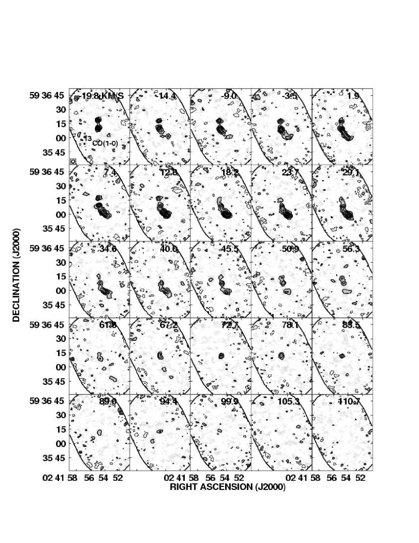
Figure 8: The redshifted half of Maffei 2’s ¹³CO(1-0) channel maps. Contours given in Figure 7.

The gas kinematics can been seen in the channel maps of ¹³CO(1–0) (Figures 7 and 8) and HCN(1–0) (9). ¹³CO(1–0) traces the velocity field of the total column density, while HCN the velocity field of the dense gas. CO emission extends from $\rm v_{LSR}\sim-$160 to +100 km s^-1 with blueshifted emission in the north. HCN is confined to velocity ranges $\rm v_{LSR}\sim-$145 to +60 km s^-1. If we assume trailing spiral arms, the northern arm is the near arm, consistent with the larger internal extinction there (Figure 2b).

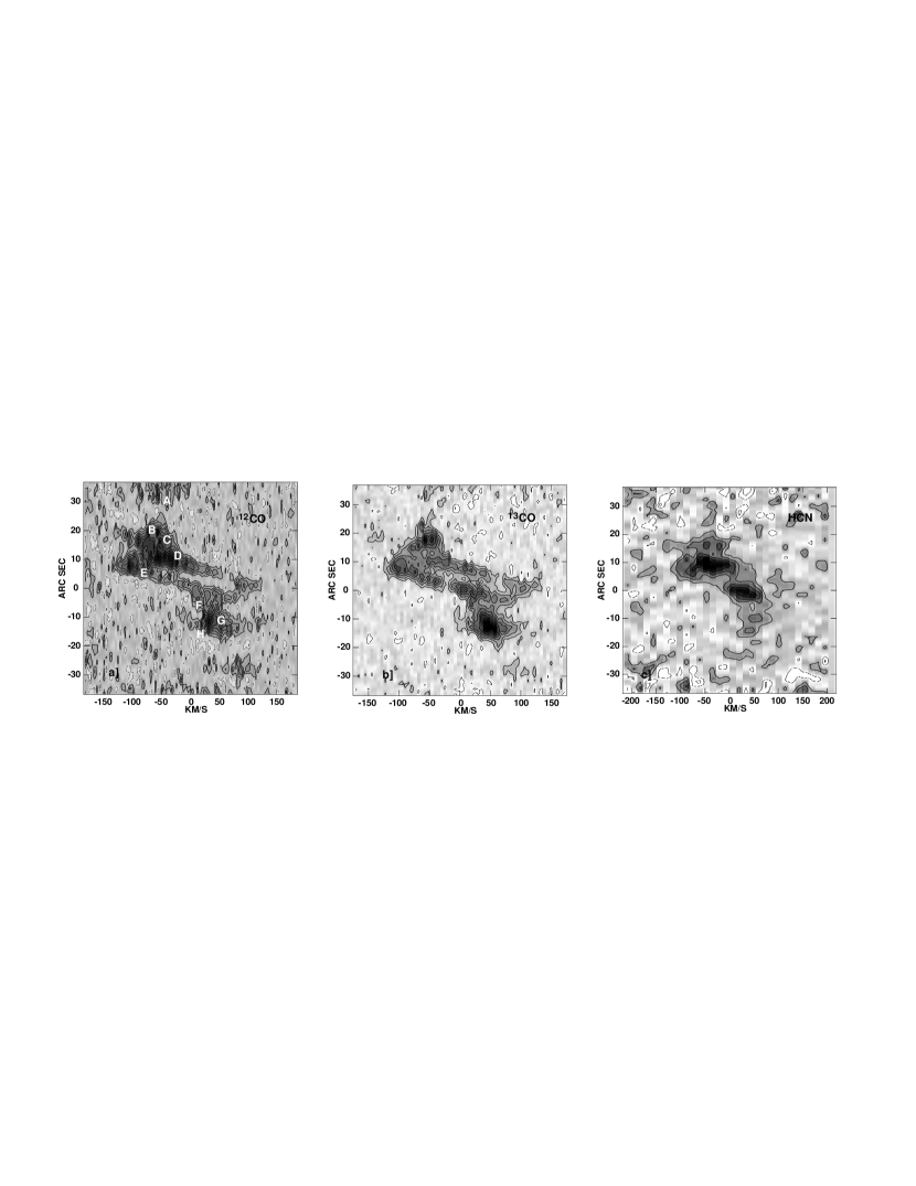
Figure 10: The a) CO(1-0), b) ¹³CO(1-0) and c) HCN(1-0) Position-Velocity (P-V) diagrams taken along the major axis of Maffei 2. The zero velocity corresponds to -20.5 km s^-1 (LSR). The zero position corresponds to 02:41:55; 59:36:10. Northeast along the galaxy is at the top of the figure. Contours are $\sim 2\sigma$. Labels in a) identify the location of each GMC in position and velocity.

Position-velocity (P-V) diagrams for Maffei 2, shown in Figure 10, were made from the cubes by averaging the central 5${}^{{}^{\prime\prime}}$ along the major axis of the galaxy ($p.a.=206^{o}$; Table Nuclear Bar Catalyzed Star Formation: ¹³CO, C¹⁸O and Molecular Gas Properties in the Nucleus of Maffei 2). We constructed major-axis P-V diagrams for CO(1-0), ¹³CO(1–0) and HCN(1–0). The CO(1–0) and ¹³CO(1–0) P-V diagrams reveal an essentially complete “parallelogram” associated with the central ring. The parallelogram has a width of $\simeq$10″, a spatial extent of 20″(160 pc in radius), and a total velocity extent of $\sim$250 km s^-1 (uncorrected for inclination). The ¹³CO-emitting gas along the central ring appears to be nearly uniform. CO(1–0), on the other hand, is asymmetric with much brighter emission at the GMC D + E starburst sites along the eastern side of the ring. The cause of the asymmetry is unclear, but since CO is so optically thick, its emissivity is more susceptible to locally elevated kinetic temperatures or other non-LTE surface effects. The uniformity of the ¹³CO is likely to be a better indicator of gas surface density in this situation. Beyond the parallelogram, the velocity field is dominated by two peaks corresponding to the ends of the molecular arms.

The velocity field of HCN(1-0) is significantly different from that of CO. The parallelogram is not apparent in the HCN P-V diagram, but instead dominated by two peaks corresponding to the intersection of the molecular arm emission and the parallelogram in the P-V diagrams. Even along the central ring, HCN has a much lower covering fraction in velocity space than CO.

6.1 Bar Model for Maffei 2

The new CO P-V diagrams (Figure 10) have sufficient spatial resolution to reveal that the “oval”-shaped pattern is actually a “parallelogram” like that observed towards the Galactic Center (Bally et al., 1988; Binney et al., 1991). The similarity of molecular gas kinematics in Maffei 2 to the Galactic Center, which is explained by gas response to a barred potential (eg. Binney et al., 1991; Huettemeister et al., 1998; Rodriguez-Fernandez et al., 2006), leads us to construct a model of barred gas response in Maffei 2.

We have modeled the gas distribution and kinematics in response to a stellar bar using an analytic weak-bar model. Such models are based on treating the dissipational nature of gas with the addition of a damping term proportional to the deviation from circular velocity (Wada, 1994; Lindblad & Lindblad, 1994; Sakamoto et al., 1999). Despite their simplicity, these model matches the structures seen in full hydrodynamical simulations with surprisingly fidelity (eg., Lindblad & Lindblad, 1994). The simplicity of an analytic bar model permits us to quickly explore a wide range of bar parameters.

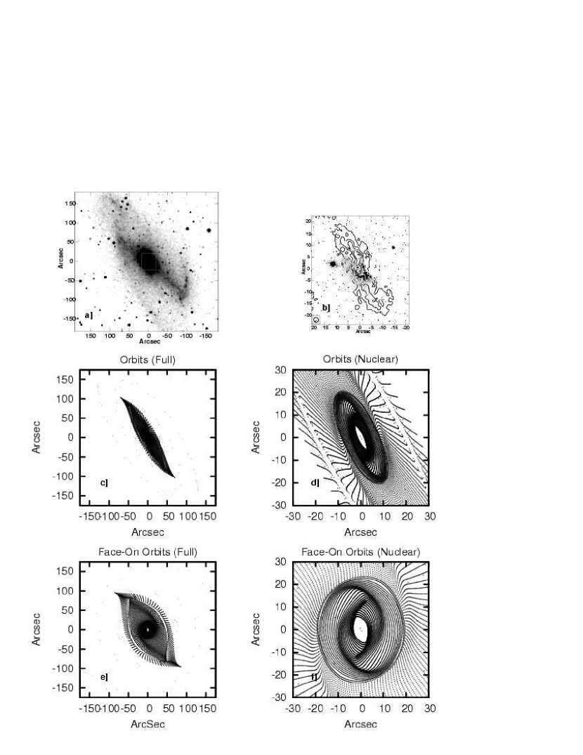
Figure 11: An epicyclic double bar model for Maffei 2. See §6.1 for a description and Table 9 for parameters. a) The 2MASS infrared K band image of Maffei 2. b) Nuclear molecular gas morphology traced by CO(1-0), showing only the 118 ($\times 1,4,8,12)$ K km s^-1 contours, overlaid off the 814W HST image. c) A model of the inner portion of the large scale bar on the same scale as a). Predicted positions of the gas peaks follow the locations of highest point density. Note that the northeastern NIR arm is tidally disturbed, and as a result the model agreement is poorer. d) A zoom in on the nuclear bar portion of the model. e) As in c) except displayed face-on. f) As in d) except viewed face-on.

Our model is based on those of Wada (1994) and Sakamoto et al. (1999), with the following modifications. (1) The gas dissipation term is extended to include azimuthal damping. This is done by adding a term, $2\mu\dot{\phi_{1}}$, to eq. (2) of Wada (1994) analogous to their eq. (1). (2) The model is extended to include both a small scale (hereafter “nuclear”) bar and a large scale bar, according to the prescription of Maciejewski & Sparke (1997, 2000). (3) The axisymmetric potential has been changed so that it generates a double Brandt rotation curve coupled in size to the two bars. The second component of the potential is required both to match the flattening of the rotation curve near the nucleus (Hurt, Turner & Ho, 1996) and to generate the necessary existence of ILRs at $\sim$5″. The size and shape of the large scale bar is set to match the NIR, CO and HI images of the galaxy (Figure 11a; Hurt et al., 1993a; Mason & Wilson, 2004; Hurt, Turner & Ho, 1996). It is assumed that the nuclear bar is co-planar with the large scale disk.

Similarities between the model and both the true gas distribution (Figure 11) and kinematics (Figure 12 & 13) are excellent. Table 9 lists the fitted model parameters. In the weak bar scheme the molecular gas is predicted to follow the sites of orbit crowding (higher density of dots in the figure). The model velocities match the observed pattern quite well. In general, the models are robust to small changes in parameters as long as two main requirements are met, (1) the combination of potential/rotation curve and bar parameters are such that there are two nuclear inner Lindblad resonances, oILR and iILR, and (2) the size scale of each bar is close to the values chosen. The first is important because it is this condition that is required for perpendicular $x_{2}$ orbits. In our barred model, the perpendicular $x_{2}$ orbits are vital to explain the large l-o-s velocities and “parallelogram” feature seen close to the center. The second point is important because it sets the scale of the features seen in the gas (ie. the $x_{1}$ orbits run between the oILR and corotation).

Our model shows gas associated with the well known $x_{1}$ and inner perpendicular $x_{2}$ orbits of barred potentials (eg. Athanassoula, 1992). A good fit for the nuclear morphology is achieved when the 4:1 ultraharmonic resonance of the nuclear bar is set equal to the oILR of the large scale bar. The pattern speed of the nuclear bar in Maffei 2 is thus much higher than the pattern speed of the larger bar, implying that the nuclear bar is decoupled from the larger scale bar. The morphology is best matched with the nuclear bar rotated $\sim 10^{o}$ clockwise (as viewed from the perspective of Figure 11e) relative to the large scale bar.

The “parallelogram” of the ¹³CO P-V diagram reveals additional information about the gas associated with the closed nuclear bar orbits. The ¹³CO parallelogram is nearly complete. This suggests that, while not obvious in the integrated intensity map due to the high inclination (though evidence is seen for it $\sim 5^{{}^{\prime\prime}}$ west of GMC E), the entire oval $x_{2}$ orbit region appears to contain molecular gas. The emission along the central ring in the P-V diagram is nearly unresolved spatially, suggesting that only a very small range of $x_{2}$ orbits are populated. Contrasts of $>$6 in column density are seen between the molecular gas associated with nuclear $x_{2}$ orbits and the very center of the galaxy, implying that the vast majority of inflowing molecular gas is trapped at the central ring and does not reach the core of the galaxy. The parallelogram suggests that a majority ($\sim$60 %) of the ¹³CO emission originates from gas residing on $x_{2}$ orbits with the rest residing on the $x_{1}$ orbits.

The observed “parallelogram” is slightly wider along the position axis than the model predicts. This suggests that the inner $x_{2}$ orbits are slightly more circular than displayed in Figure 11d. This is likely due to the limits of the epicyclic approximation at the very center of the potential. Nearly circular $x_{2}$ orbits are a common feature of the more complete hydrodynamical simulations (e.g., Piner, Stone & Teuben, 1995).

7 Molecular Clouds in the Nuclear Environment: Cloud Properties as a Function of Location

Armed with a reasonable kinematical model of the center of Maffei 2, and having identified the sites of current star formation from mm continuum maps, we can investigate the effects of environment on the properties of molecular clouds. Densities, $n_{H_{2}},$ and kinetic temperatures, T${}_{k},$ of the individual nuclear GMCs were determined by running Large Velocity Gradient (LVG) radiative transfer models with the observed intensities and line ratios as inputs (eg. Goldreich & Kwan, 1974; Scoville & Solomon, 1974; De Jong et al., 1975).

We adopt single component LVG models for the clouds. Three independent parameters, $n_{H_{2}}$, T_k and $X_{CO}$/$dv/dr$ are varied over the ranges $n_{H_{2}}$ = $10^{1}$–$10^{6}~{}cm^{-3}$, T_k = 1.5–150 K, and $X_{CO}$/$dv/dr$ = 10${}^{-3}-10^{-7.7}$ (collision coefficients are from De Jong et al., 1975). For each location, seven (eight if including HCN) distinct measurements, the two isotopic line ratios, the two $\Delta$J line ratios, the peak T_mb of the uniformly weighted CO(1-0) map and the ratio of cloud linewidth to cloud size are used to constrain the model parameters. The $\pm 1\sigma$ ranges do not include systematic uncertainties associated with changes in $X_{CO}$/$dv/dr$ or more general uncertainties related to the validity of the LVG approximation itself. Additional model solutions with $X_{CO}$/$dv/dr$ varied by a factor of $\pm$0.3 dex were determined (not shown). Increasing the velocity gradient (or correspondingly decreasing the abundance) results in an increase in derived densities by $\sim$0.3 dex and a decrease in derived T_K of $\sim$ 10 K. This variation is indicative of the sensitivity of the physical conditions to changes in the abundance or velocity gradient at the level permitted by their systematic uncertainties (§5).

In Figure 14, LVG model solutions for six locations across the central bar are displayed. Typical values of the velocity gradient for the GMCs are $\sim$ 1–2 km s^-1 pc^-1 (Table 4). We force abundance per velocity gradients of, $X_{CO}$/$dv/dr$ = $10^{-6.12}$ ($10^{-6.75}$) for ¹³CO (C¹⁸O), corresponding to [CO/H₂] $\simeq 8\times 10^{-5}$, [CO]/[¹³CO] $\simeq$ 60, [CO]/[C¹⁸O] $\simeq$ 250 (§5), and $dv/dr~{}\sim$ 1.5 km s^-1 pc^-1 (Table 4). The $\pm 1\sigma$ range for each ratio and the measured value for the CO(1-0) antenna temperature constrain parameter space.

Average densities and kinetic temperatures implied by the LVG models are $n_{H_{2}}$ $\simeq$ $10^{2.6-3.0}$ cm^-3 and T_k $\simeq$ 15–35 K. All the mapped CO lines imply a consistent set of physical conditions. Densities derived from CO tend to be nearly constant across the nuclear bar. Clouds associated with the starbursts (D and E) are slightly warmer than the others ($T_{K}\sim$ 30–40 K). By contrast, slightly cooler and denser values are derived for the quiescent gas clouds on the nuclear $x_{2}$ orbit (‘Western Ring’; Figure 14) compared to the starbursting side of the central ring (GMC E). The solutions reproduce the observed brightness temperature of the uniformly weighted CO(1–0), indicating a filling factor of unity. A unity filling factor for CO(1–0) is consistent with that estimated from ¹³CO excitation given its larger beam size. Only GMCs D and F have predicted brightness temperatures slightly lower than observed (by $\sim$50 %), which could be explained if the CO-emitting surfaces are somewhat warmer than the bulk of the gas in these clouds. The ¹³CO and C¹⁸O solutions are in excellent agreement, suggesting that the adopted relative abundances are reasonable.

HCN LVG models were also run, for levels up to J=12 (collision coefficients from Green & Thaddeus, 1974). Overlaid on Figure 14 are the observed range ($\pm 1\sigma$) for the ¹³CO(1-0)/HCN(1-0) line ratio, derived from the HCN(1-0) models. An abundance per velocity gradient, $X_{HCN}$/dv/dr = $2\times 10^{-8}$ was assumed, consistent with Galactic HCN abundances and $dv/dr$ = 1.5 km s^-1 (eg., Irvine, Goldsmith & Hjalmarson, 1987; Paglione et al., 1998). A small correction for resolved out flux has been made assuming emission is uniformly extended on scales $\mbox{$\stackrel{{\scriptstyle>}}{{{}_{\sim}}}$}30^{{}^{\prime\prime}}$. Densities derived from the HCN(1–0) line are about an order of magnitude higher than fit from the CO isotopologues: HCN is brighter than expected based on the CO-derived physical conditions. This implies that (1) these molecular clouds have a significant component of denser clumps from which the HCN originates, or (2) the HCN abundance is much larger than has been adopted. The absolute abundance of HCN is not known well enough to eliminate the second possibility, but the magnitude of the increase required ($\mbox{$\stackrel{{\scriptstyle>}}{{{}_{\sim}}}$}10\times$) makes it unlikely. The HCN data suggests that while the single-component LVG approximation yields internally consistent solutions for the optically thinner isotopologues, which sample the bulk of the molecular column density, it breaks down when including the very high density gas. The derived $n_{H_{2}}$ and T_k should then be treated as volume averages for the gas clouds traced in the isotopologues, but not necessarily the whole of the ISM. The ¹³CO/HCN would then reflect the relative fraction of very dense gas at each position (e.g., Kohno et al., 1999; Meier & Turner, 2004).

To summarize, molecular clouds in the central 300 pc of Maffei 2 averaged over $\sim$60 pc scales tend to be only modestly denser than GMCs in the disk of the Galaxy. How much denser depends on the exact velocity gradient/abundance of CO and HCN present. If the molecular gas has a velocity gradient $\sim$ 1–2 km s^-1 pc^-1, consistent temperatures and densities are obtained from the CO emitting gas, at values of $<n_{H_{2}}>~{}\simeq~{}10^{2.75}~{}cm^{-3}$ and T${}_{k}~{}\simeq~{}15$ - 35 K for all GMCs. At these densities, the CO isotopologues are subthermally excited. The HCN emission implies subclumping.

7.1 CO as a Tracer of Molecular Gas Mass: The Conversion Factor in Maffei 2

There are indications that CO(1–0) is overluminous per unit mass of $H_{2}$ gas in the nuclear regions of spiral galaxies relative to Galactic GMCs, and thus use of the Galactic conversion $X_{CO}$ can lead to overestimates of molecular gas masses in these systems. (e.g. Dahmen et al., 1998; Meier & Turner, 2001; Weiss et al., 2001; Meier & Turner, 2004). In this section, we compare several different methods of estimating molecular gas column densities to assess the validity of the conversion factor in the nucleus of Maffei 2.

7.1.1 Molecular Gas Column Densities from the Optically thin CO Isotopologues, Dust Continuum, and the Virial Theorem

Optically thin lines of CO isotopologues allow estimates of the molecular gas column density directly by summing up the emission from each molecule. These estimates depend only on the knowledge of relative CO abundance and excitation. For LTE (eg. Scoville et al., 1986),

$$N(H_{2})_{{}^{i}CO}=5.75\times 10^{17}~{}cm^{-2}~{}\frac{[T_{ex}+0.92]}{{}^{i}\nu_{G}^{2}}~{}{[~{}H_{2}~{}]\over[^{i}CO]}~{}{e^{{}^{i}T_{o}\over T_{ex}}}~{}\times~{}~{}~{}$$

$$~{}~{}~{}~{}~{}~{}~{}~{}~{}~{}~{}~{}~{}~{}~{}~{}~{}~{}~{}~{}~{}~{}~{}~{}~{}~{}~{}\left(\frac{{}^{i}\tau}{1-e^{-^{i}\tau}}\right)~{}I_{{}^{i}CO}~{}(K~{}km~{}s^{-1}).$$ (2)

where $[~{}H_{2}~{}]\over[^{i}CO]$ is the abundance of the isotopologue, ${}^{i}\nu_{G}$, ${}^{i}\tau$ and ${}^{i}T_{o}$ are the frequency (in GHz), the opacity and the characteristic temperature ($h\nu_{o}/k$) of the particular transition (${}^{i}T_{o}=5.29$ for ¹³CO(1-0) and 5.27 for C¹⁸O(1-0)). We calculate T_ex separately from the ¹³CO(2-1)/¹³CO(1-0) line ratio assuming that ${}^{13}\tau_{CO}\simeq 1$ (§5), and the C¹⁸O(2-1)/C¹⁸O(1-0) line ratio. These values and the H₂ column densities derived from them are presented in Table 8 for each peak (T_ex = 5 K is assumed for positions beyond the (2-1) primary beam). Under LTE, T_ex values turn out to be almost independent of opacity over the range of 0 – 5 (changing by $<$ 20 %) when J = 2–1/J=1–0 line ratios are around the observed value of $\sim 0.7$. Therefore systematic uncertainties in N${}_{H_{2}}$ stem primarily from uncertainties in the assumed isotopic abundances. Abundances are expected to be within a factor of $\stackrel{{\scriptstyle<}}{{{}_{\sim}}}$2 of the adopted values (§5).

Values of N${}_{H_{2}}$ range from $<0.61~{}(1.3)$–$10~{}(6.5)\times 10^{22}$ cm^-2 (Table 8), based on ¹³CO (C¹⁸O) fluxes, with corresponding mass surface densities of $\Sigma~{}\simeq~{}<$130 (280)–2200 (1400) $M_{\odot}~{}$pc^-2. Emission from the fainter C¹⁸O line does not extend to the lower column densities, otherwise the predictions of column densities from the two species agree to within a factor of 2.

Dust continuum emission has also been detected at $\lambda=$1.4 mm towards the several of the GMCs, which gives another estimate of the molecular gas mass. After accounting for the free-free contribution (Table 5), dust fluxes, $S_{1.4mm}$, range from 7–19 $\pm$3 mJy for each cloud. Assuming a gas to dust ratio of 100 by mass, the gas mass is related to the 1.4 mm dust continuum flux by (eg., Hildebrand, 1983):

$$M_{gas}(1.4~{}mm)~{}=~{}306~{}M_{\odot}\left(\frac{S_{1.4mm}}{mJy}\right)\left(\frac{D}{Mpc}\right)^{2}$$

$$~{}~{}~{}~{}~{}~{}~{}~{}~{}~{}~{}\left(\frac{\kappa_{\nu}}{cm^{2}~{}g^{-1}}\right)^{-1}\left(e^{\frac{10.56}{T_{d}}}-1\right),$$ (3)

where $\kappa_{\nu}$ is the dust absorption coefficient at this frequency, $S_{1.4mm}$ is the 1.4 mm dust flux, D is the distance and T_d is the dust temperature. The dust opacity, $\kappa_{\nu}$, at 1.4 mm is taken to be $\rm 3.1\times 10^{-3}~{}cm^{2}~{}g^{-1}$, uncertain by an estimated factor of four (Pollack et al., 1994). We adopt T${}_{d}=40$ K based on the FIR colors (Rickard & Harvey, 1983). The dust temperature applicable to the 1.4 mm observations could be lower than this if a cool dust component undetectable shortward of 160$\mu$m exists. The existence of a cooler dust component would cause us to underestimate the implied molecular gas mass. This is likely more important away from the nuclear region. Dust masses for the cloud peaks are listed in Table 8.

Virial masses can be derived from linewidths, following the treatment of Meier & Turner (2001) since the individual GMCs in the center of Maffei 2 are resolved. Virial masses are given in Table 8. They have an intrinsic uncertainty of about a factor of two due to internal cloud structure. In addition, if systematic motions such as cloud streaming motions or non-circular bar motion, are present within a single beam (almost certainly the case; §6), the linewidths due to the internal gravity will be overestimated. In short, the virial masses will be upper limits to the true cloud masses.

Finally, as a crude consistency check, a column density, ${}^{L}N_{H_{2}}$, is calculated from the LVG model derived densities, by averaging the number density over an assumed depth of $\sqrt{\theta_{a}\theta_{b}}$. These values are also recorded in Table 8. These values represent upper limits to N(H₂) if $n_{H_{2}}$ is confined to a fraction of this volume.

7.1.2 The CO Conversion Factor in Maffei 2

We can compare the three different column density estimates—optically thick CO (${}^{Xco}N_{H_{2}}$), optically thin ¹³CO (${}^{13}N_{H_{2}}$) and C¹⁸O (${}^{18}N_{H_{2}}$), and dust (${}^{D}N_{H_{2}}$) — to estimate a CO conversion factor, $X_{CO},$ for the nucleus of Maffei 2. Column densities based on the CO isotopologues (Table 8) are lower than the those derived from CO(1-0) intensities using the Galactic value of $X_{CO}$ $\simeq$ $2\times 10^{20}$ $\rm cm^{-2}$ $\rm(K~{}km~{}s^{-1})^{-1}$ (Strong et al., 1988; Hunter et al., 1997; Dame et al., 2001). Values from the thin C¹⁸O lines are $\sim$2–4 times lower than the X_CO estimates. If we require that H₂ column densities derived from opacity-corrected ¹³CO(1–0) and C¹⁸O(1–0) agree (thereby constraining $\tau_{13CO(1-0)}$) then Galactic values of the conversion factor can be reached only for [CO/C¹⁸O] $\stackrel{{\scriptstyle>}}{{{}_{\sim}}}$ 600. Given the high metallicity environment of the nucleus of Maffei 2, this seems unlikely. Away from the nucleus there is some evidence for another factor of two further decrease in the conversion factor; however, statistical uncertainties are at least this large due to weak emission and T_ex not being determined towards these locations.

Uncertainties estimated for the gas column derived from dust emission are higher than for the isotopologues, but they too tend to support lower gas columns than predicted by the Galactic $X_{CO}$. Dust-based gas masses are also lower than the $X_{CO}$ values by factors of $\sim$2–4 for the adopted dust parameters towards the detected GMCs (Table 8). Gas column densities estimated from the dust are in good agreement with the opacity corrected ¹³CO estimates except for GMC E, but trend a factor of $\sim$30 % higher than those from the C¹⁸O isotopologues. This is an indication that the uncertainty in these column densities are at least this large. While these methods are different, we do not claim they are completely independent, because there may be hidden correlations between, say, CO relative abundance and dust to gas ratio. But the dependences on metallicity and other factors such as temperature are not necessarily the same for these mass tracers. That the gas column densities estimated from the dust and C¹⁸O are both low provides additional confidence for the assertion that the gas column densities are overestimated by the Galactic value of $X_{CO}$.

Column densities obtained by averaging the virially derived masses are higher than the other methods, which is not surprising. Linewidths in the central region (particularly GMCs C, D, E and F) include two distinct components moving on completely different orbits (Figure 10), and so systematic motions within the $\sim$60 pc (line-of-sight) beam due to the bar orbits (§6.1) cause an observed linewidth larger than random gravitational motions within the clouds would imply. Because of the presence of this motion, we expect that virial methods using observed linewidths to be severe overestimates of the cloud masses.

In summary, we conclude that the conversion between ¹²CO(1-0) and H₂ column density applicable to the central region of Maffei 2 is ${}^{M2}X_{CO}$ $\simeq$0.5 –1.0 $\times 10^{20}$ $cm^{-2}~{}(K~{}km~{}s^{-1})^{-1}$, $\sim$2–4 times lower than the Galactic value, with uncertainties of $\sim$100 %.

8 A Nuclear Bar-Driven Starburst in Maffei 2

8.1 Star Formation Rates and Efficiencies

The rotation curve from the double bar model can be used to estimate dynamical masses directly without having to try to remove the non-circular velocity component (Figure 13b). The dynamical mass over the central ring is M${}_{dyn}(R=7^{{}^{\prime\prime}})=2.1\times 10^{8}~{}M_{\odot}$. The molecular mass estimated from C¹⁸O over the same region is 6.9$\times 10^{6}~{}M_{\odot}$. Dynamical masses for the central $20^{{}^{\prime\prime}}$ radius are M${}_{dyn}(20^{{}^{\prime\prime}})=7.3\times 10^{8}~{}M_{\odot}$, while the molecular mass over this region is 2.1$\times 10^{7}~{}M_{\odot}$. Molecular mass fractions are thus $\sim$3% percent over much of the central molecular bar. Molecular mass fractions scale as the distance, so the uncertainty in the distance to this galaxy (§2) can change these values by up to a factor of 2. Resonant structures, such as the molecular bar observed in the nucleus, are probably driven by the stellar potential rather than the gas.

Lyman continuum ionization rates, N_Lyc (for T${}_{e}=10^{4}$ K; e.g. Mezger & Henderson, 1967), and star formation rates based on the 89 GHz continuum are given in Table 6. To produce the total observed free-free emission across the central 30${}^{{}^{\prime\prime}}$, the excitation of 2600 effective O7 (Vacca, Garmany & Shull, 1996) stars is required. A significant fraction of this ionizing flux ($\sim 1.4\times 10^{52}~{}s^{-1}$, or $\sim$ 1400 “effective” O7 stars) arises near the two central molecular peaks (GMCs D1+E and F). Towards radio continuum sources, I, II and IV, the local star formation rates are 0.05, 0.05 and 0.04 M${}_{\odot}~{}yr^{-1}$, respectively, based on the conversion between $N_{Lyc}$ and SFR of Kennicutt (1998). These values match the star formation rate predicted from the HCN(1–0) luminosity using the relationship that Gao & Solomon (2004) have derived from large scale HCN measurements. The relationship between HCN(1–0) luminosity and star formation on 60 pc scales in Maffei 2 is the same as that observed on kpc scales in luminous infrared galaxies.

The ionization rate across the nuclear bar corresponds to a massive star formation rate of $\sim$ 0.26 M_⊙ yr^-1 with $\sim$0.14 M_⊙ yr^-1 originating from the nuclear ring. At this rate the molecular gas in the ring could sustain the current star formation rate for $\sim 5\times 10^{7}$ yrs if no gas replenishment from the arms occur. If a ZAMS Salpeter IMF with an upper (lower) mass cutoff of 100 M_⊙ (0.1 M_⊙) is adopted then a total stellar mass over the central ring of $M_{*}=5.4\times 10^{5}$ M_⊙ is generated in the current burst. These values correspond to star formation efficiencies, SFE = $M_{*}/(M_{*}+M_{H_{2}})$, of $\sim$10% over the central ring, peaking at the nuclear $x_{1}$ - $x_{2}$ orbit intersections. The SFE drops to $\stackrel{{\scriptstyle<}}{{{}_{\sim}}}$ 4% along the molecular arms, similar to Galactic disk values.

8.2 Gas Inflow, Stability and Triggered Star Formation in Maffei 2

What drives the star formation in the nucleus? Is it the large molecular gas surface density or is there evidence for a trigger that is unique to the nuclear region? What is responsible for the large concentration of nuclear gas in Maffei 2? With these observations we can address the link between star formation and molecular gas on GMC sizescales in the nuclear region of Maffei 2.

In the context of our dynamical model, the presence of the large gas mass is probably due to slow inflow along the nuclear bar (eg. Roberts et al., 1979; Athanassoula, 1992; Turner & Hurt, 1992; Regan, Vogel, & Teuben, 1997; Sheth et al., 2005). Is there sufficient gas inflow to produce the observed star formation? It is assumed that the inflowing gas will form stars, and that the star formation process is initiated at the location of the $x_{1}$-$x_{2}$ orbit intersection in the nuclear ring. Then the radial gas mass flux at this galactocentric radius determines the star formation rate. The gas mass flux is related to the average inflow velocity, $v_{inf}$, the average arm mass surface density, $\overline{\Sigma}_{arm}$, and the arm width, $w$. From the ¹³CO data $\overline{\Sigma}_{arm}~{}\simeq~{}210$ M_⊙ pc^-2 and $w\simeq 5^{{}^{\prime\prime}}$ (80 pc). Inflow velocities are determined from the bar model. Typical values are -20 to -40 km s^-1 along the bar arms. Averaged over the arm area only, $v_{r}~{}\simeq~{}$ -21 km s^-1. Adopting these values (an upper limit), a mass inflow rate, $\dot{M}_{inf}\sim 0.7$ M_⊙ yr^-1 is obtained. Since $\dot{M}_{inf}$ is a factor of $\sim$5 larger than the nuclear ring star formation rate estimated from the millimeter continuum, the inflow rate is sufficient to fuel the nuclear starburst even with modest efficiency.

Does the molecular gas form stars due to gravitational instabilities or is it directly triggered? The gravitational stability of a thin, rotating disk can be estimated from the Toomre $Q$ parameter (Safronov, 1960; Toomre, 1964). A gas disk is unstable to gravitational collapse if $Q~{}=~{}\kappa\sigma/\pi G\Sigma_{gas}<$ 1, where $\kappa$ is the epicyclic frequency, $\sigma$ is the gas velocity dispersion and $\Sigma_{gas}$ is the gas surface density. Figure 13b displays the azimuthally averaged values of $\kappa$ from the bar model together with the observed ¹³CO velocity dispersion, mass surface density, and corresponding $Q$ values. $Q$ is 8–10 across the central ring region containing the starburst and remains $>$1 over the central 30${}^{{}^{\prime\prime}}$ radius. Clearly the data are not consistent with star formation occurring in $Q<1$ gravitationally unstable gas. This is not surprising for gas in the very center of galaxies given the (1) strong noncircular motions present, (2) the failure of the thin differentially rotating disk approximation and (3) potentially strong turbulence and magnetic fields (e.g., Elmegreen, 1999; Combes, 2001; Wong & Blitz, 2002).

Another estimator for gravitational stability that may be more suitable to nuclear gas can be obtained from Elmegreen (1994). Elmegreen (1994) estimates the critical density above which gas in a ring associated with an ILR can collapse to form stars as $\rho_{crit}=0.6~{}\kappa^{2}/G$, or $n_{crit}~{}=~{}2.08\times 10^{-3}~{}\kappa^{2}$(km s^-1 kpc^-1). The epicyclic frequency at the radius of the ring is $\kappa~{}\simeq~{}2000$ km s^-1 kpc^-1 which implies ring densities must be $n_{H2}>~{}8\times 10^{3}~{}cm^{-3}$ to be unstable to collapse. From the LVG analysis we find that the average density of the CO-emitting gas along the central ring is an order of magnitude lower than this value.

A lower limit to the stability of the molecular clouds can be set by assuming the clouds remain gravitationally bound against tidal forces. A cloud of mass, $m$, will remain bound if $m~{}\mbox{$\stackrel{{\scriptstyle>}}{{{}_{\sim}}}$}~{}M(R)(r/R)^{3}$, where $M(R)$ is the total mass enclosed within a galactocentric radius, $R$, and $r$ is the size of the molecular cloud (eg., Stark et al., 1991). Clouds with densities of $n_{H_{2}}^{tidal}~{}\mbox{$\stackrel{{\scriptstyle>}}{{{}_{\sim}}}$}~{}3.6M_{M_{\odot}}(R)R_{pc}^{-3}$ remain bound. For $R$ = 80 pc and $M_{M_{\odot}}(80~{}pc)~{}=~{}1.1\times 10^{8}$ M_⊙, values applicable to Maffei 2’s nuclear ring, $n_{H_{2}}^{tidal}~{}\simeq~{}630$ cm^-3. This value is close to the densities inferred from our LVG analysis. The average molecular gas densities in the central ring are too low to be gravitationally unstable, and are likely only marginally tidally bound. Indeed, along much of the central molecular ring not associated with the sites where the arms terminate, little star formation is observed.

It appears, then, that gravitational instability is not the answer. Instead we consider the possibility that the star formation is triggered by events external to the clouds. Star formation in the nucleus of Maffei 2 is concentrated at the location of the $x_{1}$-$x_{2}$ orbit intersections indicated by our modeling. At these $x_{1}$-$x_{2}$ orbit intersection regions star formation appears to be triggered by the collision of gas flowing inward along the arms of the bar with the existing, more diffuse gas of the central ring.

We propose that the evolution of the nuclear starburst has proceeded as follows. A recent interaction between a small companion and Maffei 2 has driven a large quantity of gas into the nucleus, building up a compact central bulge seen in the NIR (Hurt et al., 1993a; Hurt, Turner & Ho, 1996). Assuming the potential generated by this compact bulge is slightly oval (a few percent is all that is necessary), it has forced the nuclear molecular gas into the bar distribution currently observed. Inflow along the nuclear $x_{1}$ orbits piles up gas at the nuclear $x_{1}-x_{2}$ orbit intersections. The interaction results in a fraction of the molecular gas going to the formation of dense cloud cores which collapse and trigger the star formation events at GMC D and just downstream of GMC F. Gas not incorporated into the dense component at these locations is then tidally sheared into the moderate density, nearly uniformly distributed ring, which in turn becomes the target for future collisions with infalling gas. As long as there is gas flowing inward the burst of star formation at the arm–ring intersection can be sustained.

This scenario provides a good framework for all of the molecular gas and millimeter continuum observed toward Maffei 2, with one exception, the star formation near GMC E. This star-forming complex is on the $x_{2}$ orbit but not at either of the $x_{1}$-$x_{2}$ intersection regions. Nor is it a strong HCN source (though some HCN emission is seen). Why is star formation occurring here? Two possibilities come to mind: (1) The star formation is triggered by the molecular gas associated with GMC E interacting with the molecular gas towards GMC D after having traversed one half of the $x_{2}$ orbit. (2) The star formation here reflects a slightly earlier epoch event associated with its passing through the southern $x_{1}$ - $x_{2}$ interaction region. It is now being seen with a time lag equal to the traversed portion of the ring divided by the orbital velocity. From the nuclear ring parameters the time lag would be $\sim$ 1 Myr. That the spectral index of the millimeter continuum is somewhat steeper towards GMC E, possibly suggesting a slightly older starburst with more evolved and less dense H II regions, may favor the latter scenario.

8.3 Comparisons of Maffei 2 with Other Nearby Nuclei

The nuclear morphology of Maffei 2 is similar to that observed in the bright nuclei of the barred galaxies, IC 342, NGC 6946 and M 83 (eg. Ishizuki et al., 1990; Regan & Vogel, 1995; Sakamoto et al., 2004) and the central molecular zone of the Galaxy (eg. Binney et al., 1991; Rodriguez-Fernandez et al., 2006). All have nuclear bar morphologies reminiscent of their large scale analogs (e.g., Athanassoula, 1992). In IC 342 and M 83, it remains somewhat ambiguous whether they are nuclear bars or just the inner portions of the large scale bar, due to a combination of having massive clusters that potentially influence the dynamics (e.g., Schinnerer et al., 2003; Crosthwaite et al., 2004; Sakamoto et al., 2004; Schinnerer et al., 2007) and low inclination, which hampers kinematic studies. Maffei 2’s kinematics leave little doubt that it is a true double bar. In fact the CO velocity field in the nucleus of Maffei 2 is perhaps the best current example of nuclear non-circular, bar motions outside our own Galactic Center. Therefore Maffei 2 can be added to NGC 6946 as confirmed double barred galaxies, but with a physical scale about three times larger. It is interesting that like NGC 6946 (and NGC 2974; Ishizuki et al., 1990; Emsellem et al., 2003; Schinnerer et al., 2006), our CO(1–0) observations imply the existence of straight shocks in nuclear bars. The inner ring and offset straight shocks do not appear to be common features of hydrodynamical models of secondary bars (eg., Shlosman & Heller, 2002; Maciejewski et al., 2002). Moreover, this conclusion seems to hold true for galaxies with both strong large scale bars (Maffei 2) and weak large scale bars (eg. NGC 6946).

These nuclear bars also influence physical conditions of the gas. Despite the presence of luminous star-forming complexes in these nuclei, emission from the lines of the CO isotopomers is dominated by subthermally excited emission from low excitation (T${}_{ex}~{}\sim 5-15$ K) gas, and that this emission represents the properties of the bulk of the molecular gas. While the ISM in Maffei 2 appears slightly warmer than IC 342 (Meier & Turner, 2001) its T_k are very close to the average properties of NGC 6946 and the outer gas lanes of the Galactic Center (Huettemeister et al., 1993; Paglione et al., 1998; Meier & Turner, 2004; Nagai et al., 2007). However, densities in the nucleus of Maffei 2 are consistently about 0.5 dex lower than NGC 6946 and the Galactic Center. We suggest this comes from Maffei 2 having a stronger nuclear bar than the other two nuclei, resulting in more dramatic disruption and redistribution of its nuclear ISM.

9 Summary

New aperture synthesis maps are presented for emission in the J=2–1 and 1–0 transitions of ¹³CO and C¹⁸O, as well as the J=1–0 lines of HCN and CO in the central arcminute ($\sim$ 1 kpc) of Maffei 2. The H₂ column density as traced by optically thin CO isotopologues is similar in morphology to what is implied from ¹²CO, except that the emission from the isotopologues is more closely confined to the two extended molecular arm ridges and more uniformly distributed across the central ring. The dense gas traced by HCN(1-0) is more confined to the center of the galaxy than the CO emitting gas.

The central molecular bar contains five main peaks that resolve into at least 17 distinct GMCs, with radii of $\sim$40–110 pc and linewidths $\stackrel{{\scriptstyle>}}{{{}_{\sim}}}$ 40 km s^-1. In the two innermost molecular cloud complexes, at galactocentric radii of $\sim 5$″ (80 pc from the dynamical center), the GMCs are distinctly nonspherical, elongated along the nuclear bar, with linewidths as large as 100 km s^-1. These GMCs are probably being tidally stretched due to the nuclear potential.

The H₂ column density for the central GMCs is $N_{H_{2}}~{}\simeq~{}4.4-10\times 10^{22}~{}cm^{-2}$ ($\overline{\Sigma}~{}\sim 950-2200$ M_⊙ pc^-2), corresponding to mean optical extinctions of $A_{v}\sim$40–100. The molecular mass within the central 20″ galactocentric radius ($\sim$300 pc) is 2.1$\times 10^{7}~{}M_{\odot}$, while the dynamical mass in the same region is M${}_{dyn}(20^{{}^{\prime\prime}})=7.3\times 10^{8}~{}M_{\odot}$. The molecular mass is only a few percent of the dynamical mass. Excitation temperatures, assuming ${}^{13}\tau(^{18}\tau)~{}\sim$ 1  ($\ll$1), are T${}_{ex}~{}\sim~{}3~{}-~{}6$ K over much of the central 500 pc for both ¹³CO and C¹⁸O. These T_ex values are low compared with the brightness temperature observed in CO ($\mbox{$\stackrel{{\scriptstyle>}}{{{}_{\sim}}}$}30$ K) indicating subthermal excitation, and that the average densities of the GMCs are probably only moderate. Single component LVG analysis of the GMCs in CO, ¹³CO, and C¹⁸O yield best-fit solutions of $n_{H_{2}}~{}\simeq~{}10^{2.75}~{}cm^{-3}$ and T${}_{kin}~{}\simeq~{}20-30$ K. Average densities estimated from the total C¹⁸O column densities are consistent with these values.

The ¹³CO and C¹⁸O lines are weaker than expected from CO(1-0), which appears to be overluminous per unit gas mass across the starburst region. Column densities derived from both C¹⁸O and 1.4 mm dust continuum emission imply that $X_{CO}$(Maf 2) is about 2–4 times lower than the Galactic value, similar to $X_{CO}$ values found for the centers of other large spirals, including our own. The weakness of the isotopologues at large galactocentric radii and in the “off-arm” spray regions of Maffei 2, suggest that in these regions either the isotopologues cease to effectively trace molecular gas or that the Galactic conversion factor overestimates the molecular column. The lack of applicability of the Galactic $X_{CO}$ to the clouds in the center of Maffei 2 is probably due to the effect of bar motions and strong tides on the structure and dynamics of these clouds.

Millimeter continuum emission reveals three prominent locations of star formation with the most intense occurring where the molecular bar intersects the nuclear ring. Lyman continuum rates of N${}_{Lyc}\sim 3$–$5\times 10^{51}$ s^-1 are implied for individual regions. The total rate for the entire nucleus is ${}_{Lyc}\sim 2.6\times 10^{52}$ s^-1, or SFR $\sim$0.26 M_⊙ yr^-1.

A P-V diagram of the nucleus of Maffei 2 shows a distinct “parallelogram” indicating molecular gas response to a barred potential. The morphological and kinematic data confirms Maffei 2 as true double barred galaxy. We suggest a bar model where the nuclear gas distribution and velocity is governed by a small nuclear bar of $r=\sim$110 pc. An upper limit to the mass inflow rate along the nuclear bar is $dM/dt~{}\mbox{$\stackrel{{\scriptstyle<}}{{{}_{\sim}}}$}~{}0.7$ M_⊙ yr^-1, enough to drive the current star formation rate seen at the end of the bar arms and populate the nuclear ring with gas. The locations of star formation and the dense gas in the central region appear to coincide with the location of the $x_{1}-x_{2}$ orbit crossings of the nuclear bar, consistent with dynamical triggering of the the star formation.

Table 1: Maffei 2 Basic Data

Characteristic	Value	Reference
Revised Hubble Class	SBb(s) pec	1
Dynamical Center	$\alpha(J2000)=02^{h}41^{m}54^{s}.90\pm 0.^{s}15~{}~{}~{}$	3
	$\delta(J2000)=+59^{o}36^{\prime}14.^{{}^{\prime\prime}}4\pm 2^{{}^{\prime\prime}}$
$\ell^{II}$,bII	136.5o,-0.3o	1
Vlsr	-30 kms-1	3
Adopted Distance	3.3 Mpc	4
Inclination Angle	67o	3
Position Angle	206o	3
M(HI)	$4.0\times 10^{8}~{}M_{\odot}$	3
M(H2)	$8.5\times 10^{8}~{}M_{\odot}$	5

References. — (1) Hurt et al. (1993a); (2) Hurt & Turner (1991); (3) Hurt, Turner & Ho (1996); (4) Fingerhut et al. (2007), See text; (5) Mason & Wilson (2004).

Table 2: Observational Data

Transition	$\nu_{o}$	Tsys	$\Delta V_{chan}$	$\nu_{band}$	Beamsize	Noise	Det.
						Level	Flux
	(GHz)	(K)	(km s-1)	(MHz)	(”;o)	(mK/mJy/Bm)	(%)
OVRO:
HCN(1-0)	88.63	300-410	13.53	128	3.8x3.3;-29o	120/10	65
13CO(1-0)	110.20	230-430	2.72	128	3.9x3.4;-76o	77/10	92
13CO(2-1)	220.40	500-1000	2.72	128	3.3x2.9;-76o	75/28	$\sim$50
C18O(1-0)	109.78	240-430	10.92	128	2.6x2.2;-84o	130/7.5	$\cdots$
C18O(2-1)	219.56	300-1000	5.46	128	1.7x1.5;-62o	150/32	$\cdots$
3.4 mm	88.92	300-410	$\cdots$	1000	2.5x2.5;0o	17/0.67	$\cdots$
2.7 mm	109.5	230-430	$\cdots$	1000	3.9x3.4;-76o	3.9/0.50	$\cdots$
1.4 mm	219.3	300-1000	$\cdots$	1000	1.7x1.5;-62o	25/2.5	$\cdots$
BIMA:
12CO(1-0)	115.27	380-1300	4.07	172	3.2x3.1;-14o	1400/0.15	105

Note. — Dates for the observations are ¹³CO(1–0), 1994 October 23–1995 January 2; ¹³CO(2–1), 1993 October 26–1994 January 13; C¹⁸O(1–0) and C¹⁸O(2–1), 1998 October 19–1999 January 5; HCN(1–0), 1999 January 28–1999 March 29; ¹²CO(1-0), 2004 March 15.

Table 3: Measured Intensities

	12CO(1-0)	HCN(1-0)	13CO(1-0)	13CO(2-1)	C18O(1-0)	C18O(2-1)
	($K~{}km~{}s^{-1}$)	($K~{}km~{}s^{-1}$)	($K~{}km~{}s^{-1}$)	($K~{}km~{}s^{-1}$)	($K~{}km~{}s^{-1}$)	($K~{}km~{}s^{-1}$)
A	$520\pm 50$	$\mbox{$\stackrel{{\scriptstyle<}}{{{}_{\sim}}}$}8.3$	$8.5\pm 0.9$	$\cdots$	$<5.4$	$\cdots$
B	$540\pm 50$	$26\pm 3$	$38\pm 4$	$\sim 4.8$	$\sim 8.7$	$\sim 5.2$
C	$780\pm 80$	$56\pm 6$	$56\pm 6$	$9.3\pm 1.8$	$23\pm 2$	$13\pm 3$
D	$1300\pm 100$	$110\pm 10$	$93\pm 9$	$73\pm 10$	$26\pm 3$	$18\pm 4$
E	$1200\pm 100$	$100\pm 10$	$120\pm 10$	$83\pm 20$	$28\pm 3$	$21\pm 4$
F	$680\pm 70$	$83\pm 8$	$85\pm 9$	$41\pm 8$	$21\pm 2$	$17\pm 3$
G	$530\pm 50$	$23\pm 2$	$63\pm 6$	$11\pm 2$	$17\pm 2$	$\mbox{$\stackrel{{\scriptstyle<}}{{{}_{\sim}}}$}3.5$
H	$170\pm 20$	$<8.3$	$\mbox{$\stackrel{{\scriptstyle<}}{{{}_{\sim}}}$}6.8$	$\cdots$	$<5.4$	$\cdots$

Note. — Uncertainties are the larger of the map uncertainty or the absolute calibration uncertainties (assuming to be 10 % for the 3 mm lines and 20 % for the 1 mm lines). Refer to Figure 2 or Table 4 for the GMC positions. Values are obtained from maps convolved to the ¹³CO(1-0) beamsize. For these lower resolution maps the GMCs are sampled at the “1” component of each GMC (except G which is sampled at G3), which corresponds approximately to the peak in the lower resolution maps.

Table 4: Giant Molecular Clouds

GMC	$\alpha,~{}\delta$	$a\times b;~{}pa$	$\Delta v_{1/2}$	$v_{o}$	Tpk	$M_{vir}$
	(02h41m;59o36${}^{{}^{\prime}}$)	($pc\times pc;^{o}$)	($km~{}s^{-1}$)	($km~{}s^{-1}$)	$(K)$	($10^{6}~{}M_{\odot}$)
A1	57.17,42.4	$51\times 36$;46	78$\pm$3	-66$\pm$1	13	34
A2	57.86,42.2	$29\times 29$;120	82$\pm$8	-59$\pm$3	9	30
A3	57.51,41.6	$52\times 31$;23	95$\pm$7	-67$\pm$3	21	47
B1	55.95,26.9	$76\times 42$;180	75$\pm$2	-89$\pm$1	9	42
B2	55.75,29.6	$55\times 41$;18	41$\pm$2	-80$\pm$1	17	10
C	55.48,24.8	$110\times 30$;26	61$\pm$1	-84$\pm$1	18	29
D1	55.14,20.7	$76\times 33$;28	84$\pm$1	-74$\pm$1	31	46
D2	54.78,24.7	$39\times 23$;34	8.6$\pm$3	-54$\pm$1	9	0.29
E	55.08,18.4	$110\times 26$;160	110$\pm$1	-79$\pm$1	19	87
F	54.86,09.6	$95\times 33$;36	51$\pm$1	-2.0$\pm$1	24	19
G1	54.39,03.2	$65\times 29$;36	47$\pm$1	20$\pm$1	17	12
G2	54.34,00.1	$44\times<17$;55	69$\pm$4	38$\pm$2	9	$<$18
G3	54.12,59.6	$69\times 29$;73	66$\pm$2	38$\pm$2	9	25
G4	53.88,57.9	$<19\times<17$;–	79$\pm$7	30$\pm$3	12	$<$14
G5	53.77,00.7	$73\times 22$;35	64$\pm$2	23$\pm$1	14	22
H1	53.76,04.7	$64\times 23$;57	18$\pm$1	14$\pm$1	12	1.7
H2	53.52,01.4	$63\times\mbox{$\stackrel{{\scriptstyle<}}{{{}_{\sim}}}$}17$;150	70$\pm$3	24$\pm$2	9	$\stackrel{{\scriptstyle<}}{{{}_{\sim}}}$21

Note. — Positions are based on fitting the uniformly weighted CO(1-0) data. Refer to Figure 2 for the locations of each GMC. Uncertainties are 1$\sigma$ from the least-squares Gaussian fits to the data. A GMC is considered unresolved if its deconvolved size is less than 1/2 of the beam minor axis.

Table 5: Millimeter/Radio Continuum Flux and Spectral Indices

Parameter	I	II	III	IV	V	Total
($\alpha_{o},\delta_{o}$)	55.09;21.0	55.10;17.6	55.14;16.0	55.17;13.5	54.54;01.8	$\cdots$
$S_{mJy}(4.885)$	14.3$\pm$0.7	19.4$\pm$1	15.2$\pm$0.8	11.4$\pm$0.6	2.7$\pm$0.1	97$\pm$5
$S_{mJy}(14.96)$	7.0$\pm$0.4	9.6$\pm$0.5	7.0$\pm$0.4	5.6$\pm$0.3	1.0$\pm$0.2	48$\pm$2
$S_{mJy}(89.96)$	5.8$\pm$0.9	5.6$\pm$0.9	$\stackrel{{\scriptstyle<}}{{{}_{\sim}}}$3.9	5.0$\pm$0.8	1.5$\pm$0.6	32$\pm$5
$S_{mJy}(110.2)$	7.0$\pm$1	$\sim$7.0	4.7$\pm$0.7	4.1$\pm$0.7	2.7$\pm$0.5	26$\pm$3
$S_{mJy}(219.3)$	19$\pm$4	21$\pm$4	10$\pm$3	$\sim$5.3	9.7$\pm$3	79$\pm$16
$\alpha^{6}_{2}$	-0.6$\pm$0.1	-0.6$\pm$0.1	-0.7$\pm$0.1	-0.6$\pm$0.1	-2.0$\pm$0.2	-0.6$\pm$0.1
$\alpha^{2}_{3.4}$	-0.1$\pm$0.1	-0.3$\pm$0.1	$<-0.33$	-0.1$\pm$0.1	0.2$\pm$0.3	-0.2$\pm$0.1
$\alpha^{2.7}_{1.4}$	1.5$\pm$0.5	$\sim 1.6$	1.1$\pm$0.6	$\sim 0.4$	1.9$\pm$0.6	2.0$\pm$0.5

Note. — Uncertainties are based on the larger of the map noise or 5% for 6 and 2 cm (Turner & Ho 1994), 15 % absolute calibration at 3 mm (larger uncertainties reflect possible errors in line removal), and 20 % at 1 mm. Upper limits are 2$\sigma$.

Table 6: Star Formation Rates

Source	${}^{ff}S_{mJy}$	$N_{Lyc}$	SFR	${}^{D}S_{mJy}$	${}^{D}M_{H_{2}}$
(1)	(2)	(3)	(4)	(5)	(6)
I	4$\pm$0.6	5$\pm$0.6	0.05$\pm$0.01	15$\pm$3	4.8$\pm$0.8
II	4$\pm$0.6	5$\pm$0.6	0.05$\pm$0.01	19$\pm$4	6.1$\pm$1.0
III	2$\pm$0.6	3$\pm$0.6	0.03$\pm$0.01	7$\pm$3	2.3$\pm$0.8
IV	3$\pm$0.6	4$\pm$0.6	0.04$\pm$0.01	$<2.5$	$<0.81$
V	$<$1.2	$<$1.6	$<$0.02	10$\pm$3	3.3$\pm$0.8
Total	20$\pm$3	26$\pm$3	0.26$\pm$0.05	50$\pm$10	16$\pm$2.6

Note. — Table columns: (1) The radio continuum sources listed in Table 5. (2) Free-free flux, ${}^{ff}S_{mJy}$, at 88.92 GHz, is derived from the spectral fits (Figure 4). (3) N_lyc is the number of ionizing photons in units of $10^{51}~{}s^{-1}$, or $\sim 100$ O7 stars (Vacca, Garmany & Shull, 1996) implied by ${}^{ff}S_{mJy}$. (4) SFR is the star formation rate in units of $M_{\odot}~{}yr^{-1}$, based on the conversion from N_Lyc to SFR of Kennicutt (1998). (5) Thermal dust flux, ${}^{D}S_{mJy}$ at 219.3 GHz is derived from the spectral fits (Figure 4). (6) ${}^{D}M_{H_{2}}$ is the total mass in units of $10^{6}~{}M_{\odot}$ implied from the dust flux, ${}^{D}S_{mJy}$, assuming a gas-to-dust ratio of 100.

Table 7: Observed Line Ratios

GMC	$\rm\frac{{}^{12}CO(1-0)}{{}^{13}CO(1-0)}$	$\rm\frac{{}^{12}CO(1-0)}{C^{18}O(1-0)}$	$\rm\frac{{}^{13}CO(1-0)}{C^{18}O(1-0)}$	$\rm\frac{{}^{12}CO(1-0)}{HCN(1-0)}$	$\rm\frac{{}^{13}CO(2-1)}{{}^{13}CO(1-0)}$	$\rm\frac{C^{18}O(2-1)}{C^{18}O(1-0)}$
A	$62\pm$20	$>96$	$>1.6$	$>63$	$\cdots$	$\cdots$
B	$14\pm$2	$\sim 95$	$\sim 6.7$	$21\pm$4	$\sim$0.24	$\sim$0.90
C	$14\pm$2	$34\pm$7	$2.5\pm$0.4	$14\pm$2	$0.18\pm$0.05	$0.56\pm$0.1
D	$14\pm$2	$50\pm$6	$3.7\pm$0.5	$12\pm$2	$0.77\pm$0.2	$0.68\pm$0.2
E	$10\pm$1	$41\pm$4	$4.0\pm$0.5	$12\pm$2	$0.75\pm$0.2	$0.78\pm$0.2
F	$7.8\pm$1	$32\pm$5	$4.1\pm$0.7	$8.1\pm$1	$0.51\pm$0.1	$0.79\pm$0.2
G	$8.4\pm$1	$31\pm$6	$3.8\pm$0.9	$23\pm$5	$0.28\pm$0.07	$\mbox{$\stackrel{{\scriptstyle<}}{{{}_{\sim}}}$}0.82$
H	$\sim 25$	$>31$	$>1.3$	$>20$	$\cdots$	$\cdots$

Note. — Based on the resolution of the ¹³CO(1-0) data. No corrections for differences in resolved out flux have been included.

Table 8: CO Conversion Factor

	13Tex	${}^{13}N_{H_{2}}$	18Tex	${}^{18}N_{H_{2}}$	${}^{Xco}N_{H_{2}}$	${}^{D}N_{H_{2}}$	${}^{V}N_{H_{2}}$	${}^{L}N_{H_{2}}$	$\frac{{}^{MW}X_{CO}}{{}^{13}X_{co}}$	$\frac{{}^{MW}X_{CO}}{{}^{18}X_{co}}$
(1)	(2)	(3)	(4)	(5)	(6)	(7)	(8)	(9)	(10)	(11)
A	[5.0]	$\sim 0.77$	[5.0]	$<1.3$	10$\pm$1.0	$\cdots$	130	$\cdots$	$\sim$13	$>7.7$
B	$3.1\pm 1.0$	$4.4\pm 0.5$	$\sim 6.7$	$\sim$2.0	11$\pm$1.0	$\cdots$	51	$\cdots$	$2.5\pm 0.3$	$\sim$5.5
C	$2.9\pm 0.9$	$7.7\pm 0.8$	$4.8\pm 1.6$	$5.5\pm 0.6$	16$\pm$1.6	$\cdots$	45	11	$2.1\pm 0.3$	$2.9\pm 0.4$
D	$6.1\pm 2.3$	$8.2\pm 0.8$	$5.4\pm 1.8$	$6.1\pm 0.6$	26$\pm$2.6	$8\pm 2$	71	11	$3.2\pm 0.4$	$4.3\pm 0.6$
E	$6.0\pm 2.3$	$10\pm 1.0$	$5.9\pm 2.0$	$6.5\pm 0.7$	24$\pm$2.4	11$\pm$3	150	14	$2.4\pm 0.3$	$3.5\pm 0.5$
F	$4.5\pm 1.5$	$7.9\pm 0.8$	$6.0\pm 2.0$	$4.9\pm 0.5$	14$\pm$1.4	$<$1.4	47	14	$1.8\pm 0.2$	$2.9\pm 0.4$
G	$3.4\pm 1.1$	$6.8\pm 0.7$	$\mbox{$\stackrel{{\scriptstyle<}}{{{}_{\sim}}}$}6.2$	$\mbox{$\stackrel{{\scriptstyle<}}{{{}_{\sim}}}$}4.0$	10$\pm$1.0	5.6$\pm$2	$>75$	11	$1.5\pm 0.2$	$\mbox{$\stackrel{{\scriptstyle>}}{{{}_{\sim}}}$}2.5$
H	[5.0]	$\mbox{$\stackrel{{\scriptstyle<}}{{{}_{\sim}}}$}0.61$	[5.0]	$<1.3$	3.4$\pm$0.3	$\cdots$	$\mbox{$\stackrel{{\scriptstyle<}}{{{}_{\sim}}}$}53$	$\cdots$	$\mbox{$\stackrel{{\scriptstyle>}}{{{}_{\sim}}}$}5.6$	$>2.6$

Note. — Column densities are in units of $10^{22}$ cm^-2 and have been corrected for resolved flux assuming the emission is uniformly distributed over 30${}^{{}^{\prime\prime}}$ and temperatures are in units of K. Uncertainties reflect only statistical uncertainties in the intensities and do not include (larger) systematic uncertainties. Table columns: (1) the molecular peaks; (2) the excitation temperature derived from the ¹³C)(2–1)/¹³CO(1–0) line ratio, assuming $\tau_{13CO(1-0)}\simeq 1$ (§5); (3) the H₂ column density, N${}_{H_{2}}$, derived from the ¹³CO(1–0) line intensity assuming ¹³T_ex and $\tau_{13CO(1-0)}\simeq 1$; (4) and (5) as in (2) and (3) except from C¹⁸O with $\tau_{C18O(1-0)}\ll 1$; (6) N${}_{H_{2}}$ derived assuming a Galactic conversion factor of $2\times 10^{20}(Kkms^{-1})^{-1}cm^{-2}$ (eg., Strong et al., 1988; Hunter et al., 1997; Dame et al., 2001); (7) N${}_{H_{2}}$ estimated by averaging the gas mass estimated from dust emission in Table 6 over the 1.4 mm beamsize (Figure 3); (8) N${}_{H_{2}}$ estimated by averaging the virial mass over the cloud area, $\Sigma_{i}^{V}M_{i}/\Sigma_{i}A_{i}$ for each cloud component (Table 4); (9) N${}_{H_{2}}$ estimated by averaging the LVG derived density over the beamsize, assuming a third dimension of $\sqrt{\theta_{a}\theta_{b}}$; (10) the ratio of N${}_{H_{2}}$ calculated from the Galactic conversion factor to that from ¹³CO; (11) the ratio of N${}_{H_{2}}$ calculated from the Galactic conversion factor to that from C¹⁸O.

Table 9: Maffei 2 Bar Model Parameters

Characteristic	Value
position angle …………………..	29o
$i$	67o
$\theta_{main}$	-17o
$\Omega_{main}$	40 km s-1 kpc-1
$\Omega_{nuc}$	135 km s-1 kpc-1
$\theta_{nuc}$	7o
${}^{main}r_{max}$	3.6 kpc
${}^{main}v_{max}$	172 km s-1
${}^{nuc}r_{max}$	155 pc
${}^{nuc}v_{max}$	90 km s-1
nmain	1.0
nnuc	3.25
$\epsilon_{main}$	0.125
$\epsilon_{nuc}$	0.075
$\lambda$	0.125
$\mu$	0.1875

Figure 1: Integrated intensity of CO isotopologues in Maffei 2. a) CO(1-0), with contour levels of 10.0 Jy/beam km s^-1 (70 K km s^-1, $\sim 3\sigma$). b) ¹³CO(1-0), with contour levels of 0.70 Jy/beam km s^-1 (5.4 K km s^-1, $\sim 3\sigma$). c) C¹⁸O(1-0), with contour levels of 0.70 Jy/beam km s^-1 (5.4 K km s^-1, $\sim 3\sigma$). d) HCN(1-0) with contour levels of 0.70 Jy/beam km s^-1 (8.3 K km s^-1, $\sim 2\sigma$). e) ¹³CO(2-1) with contour levels of 2.5 Jy/beam km s^-1 (4.8 K km s^-1, $\sim 3\sigma$). f) C¹⁸O(2-1) with contour levels of 2.5 Jy/beam km s^-1 (4.9 K km s^-1, $\sim 2\sigma$). All transitions have been convolved to the resolution of the ¹³CO(1-0) transitions ($3.^{{}^{\prime\prime}}9\times 3.^{{}^{\prime\prime}}4$), shown in panel a).

Figure 2: a) Uniformly weighted integrated intensity maps of CO(1-0) in Maffei 2. The grayscale is in square root stretch ranging from 4.0 Jy bm^-1 km s^-1 (95 K km s^-1) to 60 Jy bm^-1 km s^-1 (1400 K km s^-1), for a $2.^{{}^{\prime\prime}}1\times 1.^{{}^{\prime\prime}}9$ beam. b) The CO(1–0) map overlaid on the HST F814W image of the nucleus. Only contours 118 K km s^-1 $\times(1,4,8,12,16)$ are shown. The cross marks the location of the dynamical center (Table Nuclear Bar Catalyzed Star Formation: ¹³CO, C¹⁸O and Molecular Gas Properties in the Nucleus of Maffei 2). c) The CO(1–0) map with locations of the fitted GMCs (Table 4) labeled. Contours are the same as a). d) A zoom in on the central region of the molecular bar. CO(1-0) is in contours (steps of 118 K km s^-1) overlaid on the 89 GHz continuum image (grayscale). Radio continuum (2 cm) source identifications of Tsai et al. (2006) are labeled with the symbols given in the legend. Symbol sizes are proportional to the 6 cm peak flux (1 mJy bm^-1 = 1${}^{{}^{\prime\prime}}$; Tsai et al., 2006). The green cross marks the location of the dynamical center.

Figure 3: Radio and millimeter continuum maps of the nucleus of Maffei 2. Contours are $\pm 2^{n/2}$, n=0,1, 2… times the given lowest contour level. Dashed lines are negative contours. a) 2 cm map of Turner & Ho (1994), with the lowest contour at 0.45 mJy beam^-1 (2$\sigma$). Roman numerals identify the five major continuum sources. b) The 89 GHz (3.4 mm) map contoured in steps of 1.2 mJy beam^-1 (2$\sigma$). Line contamination from HCN(1-0) and HCO⁺(1-0) has been removed. c) The 110 GHz (2.7 mm) map contoured in steps of 1.0 mJy beam^-1 (2$\sigma$). Line contamination from ¹³CO(1-0) has been removed. d) The 219 GHz (1.4 mm) map convolved to the resolution of the 110 GHz map. The lowest contour is 6.0 mJy beam^-1 (2$\sigma$). Beamsizes are indicated at the bottom left of each map, and in Table 2.

Figure 4: Spectral energy distributions for the millimeter continuum radio sources in Maffei 2. Data are fit with synchrotron (dashed line, $\alpha=-0.7$), free-free (dotted line, $\alpha=-0.1$) and dust (dot-dashed line, $\alpha=+3.5$) emission components (see text). The cross in Source III represents an upper limit. Triangles mark the contribution of the compact emission towards each source from higher resolution images (Tsai et al., 2006).

Figure 5: CO and HCN line ratios in Maffei 2. For comparison the ¹³CO(1-0) integrated intensity is overlaid on all planes in linear contours of 2.0 Jy/beam km s^-1 (15 K km s^-1). The resolution of all the ratio maps is $3.^{{}^{\prime\prime}}9\times 3.^{{}^{\prime\prime}}4$. The greyscale range of the ratio is noted in the wedge at the top of each panel. (a) CO(1-0)/¹³CO(1-0). (b) CO(1-0)/C¹⁸O(1-0). (c) CO(1-0)/HCN(1-0). (d) ¹³CO(2-1)/¹³CO(1-0). (e) C¹⁸O(2-1)/C¹⁸O(1-0). (f) ¹³CO(1-0)/C¹⁸O(1-0).

Figure 6: Average peak T_mb ratios for selected regions along the central ring of the P-V diagram. The schematic representation of the P-V diagram has the same geometry as Figure 10. The letters in parentheses in the upper left label the primary molecular peak in each region.

Figure 7: The blueshifted half of Maffei 2’s ¹³CO(1-0) channel maps. Contours are multiples of 30 mJy/beam ( $2\sigma$). The beamsize is given in the bottom left of the first plane.

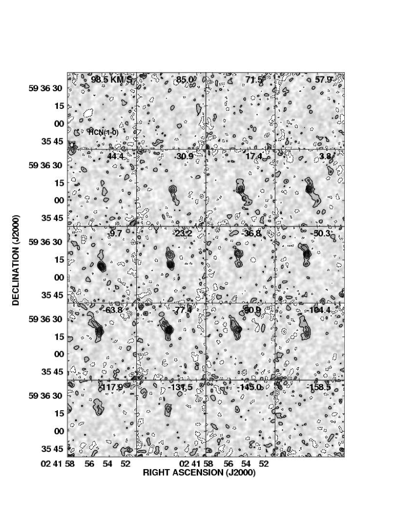
Figure 9: Maffei 2 HCN(1-0) channel maps. Contours are in increments of the $2\sigma$ value, 20 mJy/beam. The beamsize is given in the bottom left of the first plane.

Figure 12: The nuclear velocity field of Maffei 2. a) The ¹³CO(1-0) position-velocity diagram taken along the major axis (Figure 10b). b) The predicted P-V diagram for the nuclear bar on the same scale as a), showing the well known ’parallelogram’ characteristic of barred motion. Color coding shows the portion of the velocity field associated with each of the components labeled in c). c) Regions of high point density correspond to predicted (and observed) regions of gas concentration. The three main regions of predicted gas concentration are color coded—the northern and southern arms are green and blue, respectively and the central ring is pink.

Figure 13: Rotation curve of Maffei 2. a) The model rotation curve (thick red line) and observed HI rotation curve (red errorbars; Hurt, Turner & Ho, 1996) is displayed. Blue (yellow) dot-dashed lines correspond to the pattern speeds of the nuclear (main) bar. Associated resonance curves are labeled. b) A plot of dynamical properties as a function of galactocentric radius based on the modeled rotation curve. Shown are the azimuthally averaged observed velocity dispersion (green), molecular gas surface density (dark blue) from ¹³CO(1–0) assuming T_ex = 5 K and an $\tau$ = 1 (see text), epicyclic frequency (pink), implied enclosed dynamical mass (light blue) and Toomre’s Q (see text) (red). Units for each curve is given in the figure.

Figure 14: LVG model solutions for six locations across the nucleus. Abundances per velocity gradient, $X_{CO}/dv/dr$, between $10^{-7.7}-10^{-3}$ have been modeled. ${}^{i}X_{CO}\simeq$ $8\times 10^{-5}$ for [CO] / [H₂], (1/60)($8\times 10^{-5}$) for [¹³CO] / [H₂], (1/250) ($8\times 10^{-5}$) for [C¹⁸O] / [H₂], and a velocity gradient of 1 km s^-1 pc^-1 are assumed (§7.1.1). Solutions are based on the ¹³CO(1-0) resolution. Line ratios have been corrected for resolved-out flux. Contours represent the 1$\sigma$ confidence solutions. Red contours display the isotopic line ratios (thick: CO(1–0)/¹³CO(1–0); thin: CO(1–0)/C¹⁸O(1–0)) and blue contours the $\Delta$J line ratios (thick: ¹³CO(2–1)/¹³CO(1–0); thin: C¹⁸O(2–1)/C¹⁸O(1–0)). Green contours display the allowed parameter space based on the ¹³CO(1–0)/HCN(1–0) line ratio, assuming the filling factor of the HCN(1-0) emission is equal to that of the ¹³CO and C¹⁸O emission. $X_{HCN}/dv/dr~{}=~{}2.1\times 10^{-8}$, is assumed, consistent with a Galactic Center HCN abundance and a velocity gradient of $\sim$ 1 km s^-1 pc^-1 (eg., Paglione et al., 1998). The yellow line marks the CO(1–0) peak brightness temperature assuming a filling factor of unity for the uniformly weighted beamsize. Crosses mark the adopted best fit solutions.

References

- Athanassoula (1992) Athanassoula, E. 1992, MNRAS, 259, 328
- Bally et al. (1988) Bally, J., Stark, A. A., Wilson, R. W. & Henkel, C. 1988, ApJ, 324, 223
- Binney et al. (1991) Binney, J., Gerhard, O. E., Stark, A. A., Bally, J. & Uchida, K. I. 1991, MNRAS, 252, 210
- Buta & McCall (1983) Buta, R. J. & McCall, M. L. 1983, MNRAS, 205, 131
- Buta & McCall (1999) Buta, R. J. & McCall, M. L. 1999, ApJ, 124, 33
- Combes (2001) Combes, F. 2001, ASP Conf. Ser. 249: The Central Kiloparsec of Starbursts and AGN: The La Palma Connection, 249, 475
- Crosthwaite et al. (2004) Crosthwaite, L. P., Turner, J. L., Beck, S. C., & Meier, D. S. 2004, Bulletin of the American Astronomical Society, 36, 1387
- Dahmen et al. (1998) Dahmen, G., Hüttemeister, S., Wilson, T. L., & Mauersberger, R. 1998, A&A, 331, 959
- Dame et al. (2001) Dame, T. M., Hartmann, D., & Thaddeus, P. 2001, ApJ, 547, 792
- Davidge & van den Bergh (2001) Davidge, T. J. & van den Bergh, S. 2001, ApJ, 553, L133
- De Jong et al. (1975) De Jong, T., Chu, S.-I. & Dalgarno, A. 1975, ApJ, 199, 69
- Dumke et al. (2001) Dumke, M., Nieten, Ch., Thuma, G., Wielebinski, R. & Walsh, W. 2001, A&A, 373, 853
- Elmegreen (1994) Elmegreen, B. G. 1994, ApJ, 425, L73
- Elmegreen (1999) Elmegreen, B. G. 1999, Star Formation 1999, Proceedings of Star Formation 1999, held in Nagoya, Japan, June 21 - 25, 1999, Editor: T. Nakamoto, Nobeyama Radio Observatory, p. 3-5, 3
- Emsellem et al. (2003) Emsellem, E., Goudfrooij, P., & Ferruit, P. 2003, MNRAS, 345, 1297
- Englmaier & Shlosman (2004) Englmaier, P., & Shlosman, I. 2004, ApJ, 617, L115
- Fingerhut et al. (2007) Fingerhut, R. L., Lee, H., McCall, M. L., & Richer, M. G. 2007, ApJ, 655, 814
- Fingerhut et al. (2003) Fingerhut, R. L., McCall, M. L., De Robertis, M., Kingsburgh, R. L., Komljenovic, M., Lee, H., & Buta, R. J. 2003, ApJ, 587, 672
- Frerking et al. (1982) Frerking, M. A., Langer, W. D. & Wilson, R. W. 1982, ApJ, 262, 59
- Friedli & Martinet (1993) Friedli, D. & Martinet, L. 1993, A&A, 277, 27
- Gao & Solomon (2004) Gao, Y., & Solomon, P. M. 2004, ApJ, 606, 271
- Goldreich & Kwan (1974) Goldreich, P. & Kwan, J. 1974, ApJ, 189, 441
- Goldsmith, Bergin & Lis (1997) Goldsmith, P. F., Bergin, E. A., & Lis, D. C. 1997, ApJ, 491, 615
- Green & Thaddeus (1974) Green, S. & Thaddeus, P. 1974, ApJ, 191, 653
- Helfer & Blitz (1993) Helfer, T. T. & Blitz, L. 1993, ApJ, 419, 86
- Helfer & Blitz (1997) Helfer, T. T. & Blitz, L. 1997, ApJ, 478, 233
- Heller et al. (2001) Heller, C., Shlosman, I., & Englmaier, P. 2001, ApJ, 553, 661
- Henkel et al. (2000) Henkel, C., Mauersberger, R., Peck, A. B., Falcke, H. & Hagiwara, Y. 2000, A&A, 361, L45
- Henkel et al. (1994) Henkel, C., Wilson, T. L., Langer, N., Chin, Y.-N., & Mauersberger, R. 1994, “The Structure and Content of Molecular Clouds”, eds. Wilson, T. L. & Johnston, K. J., (Springer-Verlag:Berlin) pg. 72
- Hildebrand (1983) Hildebrand, R. H. 1983, QJRAS, 24, 267
- Huettemeister et al. (1998) Huettemeister, S., Dahmen, G., Mauersberger, R., Henkel, C., Wilson, T. L., & Martin-Pintado, J. 1998, A&A, 334, 646
- Huettemeister et al. (1993) Huettemeister, S., Wilson, T. L., Bania, T. M., & Martin-Pintado, J. 1993, A&A, 280, 255
- Hunter et al. (1997) Hunter, S. D. et al. 1997, ApJ, 481, 205
- Hurt (1993) Hurt, R. L. 1993, PhD thesis(University of California, Los Angeles)
- Hurt et al. (1993a) Hurt, R. L., Merrill, K. M., Gatley, I., & Turner, J. L. 1993a, AJ, 105, 121
- Hurt & Turner (1991) Hurt, R. L., & Turner, J. L. 1991, ApJ, 377, 434
- Hurt, Turner & Ho (1996) Hurt, R. L., Turner, J. L. & Ho, P. T. P. 1996, ApJ, 466, 135
- Hurt et al. (1993b) Hurt, R. L., Turner, J. L., Ho, P. T. P. & Martin, R. N. 1993b, ApJ, 404, 602 1991, ApJ, 377, 434
- Irvine, Goldsmith & Hjalmarson (1987) Irvine, W. M., Goldsmith, P. F. & Hjalmarson, A. 1987, Interstellar Processes, ed. Hollenbach, D. J., & Thronson, H. A., (Kluwer:Dordrecht), 561
- Ishiguro et al. (1989) Ishiguro, M. et al. 1989, ApJ, 344, 763
- Ishizuki et al. (1990) Ishuzuki, S., Kawabe, R., Ishiguro, M., Okumura, S. K., Morita, K.-I., Chikada, Y., & Kasuga, T. 1990, Nature, 344, 224
- Ivanov et al. (1999) Ivanov, V. D., Alonso-Herraro, A., Rieke, M. J. & McCarthy, D. AJ, 118, 826
- Karachentsev (2005) Karachentsev, I. D. 2005, AJ, 129, 178
- Karachentsev et al. (1997) Karachentsev, I., Drozdovsky I., Kajsin, S. Takalo, L. O. Heinämäki, P. & Valtonen, M. 1997, A&AS, 124, 559
- Karachentsev et al. (2003) Karachentsev, I. D., Sharina, M. E., Dolphin, A. E., & Grebel, E. K. 2003, A&A, 408, 111
- Karachentsev & Tikhonov (1993) Karachentsev, I. D., & Tikhonov, N. A. 1993, A&AS, 100 227
- Karachentsev & Tikhonov (1994) Karachentsev, I. D., & Tikhonov, N. A. 1994, A&A, 286, 718
- Kennicutt (1998) Kennicutt Jr., R. C. 1998, ARA&A, 36, 189
- Knapen (2005) Knapen, J. H. 2005, “Fueling and Morphology of Central Starbursts”, AIP Conf. Proc. 783: The Evolution of Starbursts, 783, 171
- Kohno et al. (1999) Kohno, K., Kawabe, R., & Vila-Vilaró, B. 1999, ApJ, 511, 157
- Krismer, Tully & Gioia (1995) Krismer, M., Tully, R. B. & Gioia, I. M. 1995, AJ, 110, 1584
- Langer & Penzias (1990) Langer, W. D. & Penzias, A. A. 1990, ApJ, 357, 477
- Lindblad & Lindblad (1994) Lindblad, P. O. & Lindblad, P. A. B. 1994, “Physics if the Gaseous and Stellar Disks of the Galaxy”, ed. King, I. A.S.P. vol 66, (ASP:San Fransisco), 29
- Luppino & Tonry (1993) Luppino, G. A. & Tonry, J. L. 1993, ApJ, 410, 81
- Maciejewski & Sparke (2000) Maciejewski, W., & Sparke, L. S. 2000, MNRAS, 313, 745
- Maciejewski & Sparke (1997) Maciejewski, W., & Sparke, L. S. 1997, ApJ, 484, L117
- Maciejewski et al. (2002) Maciejewski, W., Teuben, P. J., Sparke, L. S., & Stone, J. M. 2002, MNRAS, 329, 502
- Maffei (1968) Maffei, P. 1968, PASP, 80, 618
- Mason & Wilson (2004) Mason, A. M., & Wilson, C. D. 2004, ApJ, 612, 860
- McCall (1989) McCall, M. L. 1989, AJ, 97, 1341
- Meier & Turner (2001) Meier, D. S. & Turner, J. L. 2001, ApJ, 551, 687
- Meier & Turner (2004) Meier, D. S., & Turner, J. L. 2004, AJ, 127, 2069
- Meier & Turner (2005) Meier, D. S., & Turner, J. L. 2005, ApJ, 618, 259
- Meier, Turner & Hurt (2000) Meier, D. S., Turner, J. L. & Hurt, R. L. 2000, ApJ, 531, 200
- Mezger & Henderson (1967) Mezger, P. G. & Henderson, A. P. 1967, ApJ, 147, 471
- Milam et al. (2005) Milam, S. N., Savage, C., Brewster, M. A., Ziurys, L. M., & Wyckoff, S. 2005, ApJ, 634, 1126
- Nagai et al. (2007) Nagai, M., Tanaka, K., Kamegai, K., & Oka, T. 2007, PASJ, 59, 25
- Padin et al. (1991) Padin, S., Scott, S. L., Woody, D. P., Scoville, N. Z., Seling, T. V., Finch, R. P., Ciovanine, C. J., & Lowrance, R. P. 1991, PASP, 103, 461
- Paglione et al. (1998) Paglione, T.A.D., Jackson, J.M., Bolatto, A. D. & Heyer, M. H. 1998, ApJ, 493, 680
- Petitpas & Wilson (2003) Petitpas, G. R., & Wilson, C. D. 2003, ApJ, 587, 649
- Piner, Stone & Teuben (1995) Piner, B. G., Stone, J. M. & Teuben, P. J. 1995, ApJ, 449, 508
- Pollack et al. (1994) Pollack, J. B., Hollenbach, D., Beckwith, S., Simonelli, D. P., Roush, T. & Fong, W. 1994, ApJ, 421, 615
- Regan & Vogel (1995) Regan, M. W., & Vogel, S. N. 1995, ApJ, 452, L21
- Regan, Vogel, & Teuben (1997) Regan, M. W., Vogel, S. N., & Teuben, P. J. 1997, ApJ, 482, 143
- Rickard & Harvey (1983) Rickard, L. J. & Harvey, P. M. 1983, ApJ, 268, L7
- Rickard, Turner & Palmer (1977) Rickard, L. J., Turner, B. E. & Palmer, P. 1977, ApJ, 218, L51
- Rieu et al. (1991) Rieu-N-Q., Henkel, C., Jackson, J. M., & Mauersberger, R. 1991, A&A, 241, L33
- Rieu et al. (1992) Rieu, N-Q., Jackson, J. M., Henkel, C., Truong, B. & Mauersberger, R. 1992, ApJ, 399, 521
- Roberts et al. (1979) Roberts, W. W., Jr., Huntley, J. M., & van Albada, G. D. 1979, ApJ, 233, 67
- Rodriguez-Fernandez et al. (2006) Rodriguez-Fernandez, N. J., Combes, F., Martin-Pintado, J., Wilson, T. L., & Apponi, A. 2006, A&A, 455, 963
- Safronov (1960) Safronov, V. S. 1960, Annales d’Astrophysique, 23, 979
- Saha, Claver, & Hoessel (2002) Saha, A., Claver, J., & Hoessel, J. G. 2002, AJ, 124, 839
- Sakamoto et al. (2004) Sakamoto, K., Matsushita, S., Peck, A. B., Wiedner, M. C., & Iono, D. 2004, ApJ, 616, L59
- Sakamoto et al. (1999) Sakamoto, K., Okumura, S. K., Ishizuki, S. & Scoville, N. Z. 1999, ApJS, 124, 403
- Sargent et al. (1985) Sargent, A. I., Sutton, E. C., Masson, C. R., Lo, K. Y. & Phillips, T. G. 1985, ApJ, 289, 150
- Schinnerer et al. (2006) Schinnerer, E., Böker, T., Emsellem, E. & Lisenfeld, U. 2006, ApJ, 649, 181
- Schinnerer et al. (2003) Schinnerer, E., Böker, T., & Meier, D. S. 2003, ApJ, 591, L115
- Schinnerer et al. (2007) Schinnerer, E., Böker, T., Meier, D. S. & Calzetti, D. 2007, Science, submitted
- Scoville et al. (1994) Scoville, N. Z., Carlstrom, J., Padin, S., Sargent, A., Scott, S. & Woody, D. 1994, Astronomy with Millimeter and Submillimeter Wave Interferometry, IAU Colloquium 140, ASP Conference Series, Vol. 59, 1994, M. Ishiguro and J. Welch, Eds., p.10
- Scoville et al. (1986) Scoville, N. Z., Sargent, A. I., Sanders, D. B., Claussen, M. J., Masson, C. R., Lo, K. Y., & Phillips, T. G. 1986, ApJ, 303, 416
- Scoville & Solomon (1974) Scoville, N. Z. & Solomon, P. M. 1974, ApJ, 187, L67
- Scoville et al. (1987) Scoville, N. Z., Yun, M. S., Clemens, D. P., Sanders, D. B. & Waller 1987, ApJS, 63, 821
- Sheth et al. (2005) Sheth, K., Vogel, S. N., Regan, M. W., Thornley, M. D., & Teuben, P. J. 2005, ApJ, 632, 217
- Shlosman, Frank & Begelman (1989) Shlosman, I., Frank, J. & Begelman, M. C. 1989, Nature, 338, 45
- Shlosman & Heller (2002) Shlosman, I., & Heller, C. H. 2002, ApJ, 565, 921
- Sorai et al. (2002) Sorai, K., Nakai, N., Kuno, N., & Nishiyama, K. 2002, PASJ, 54, 179
- Stark et al. (1991) Stark, A. A., Bally, J., Gerhard, O. E., & Binney, J. 1991, MNRAS, 248, 14P
- Strong et al. (1988) Strong et al. 1988, A&A, 207,1
- Takano et al. (2000) Takano, S., Nakai, N., Kawaguchi, K. & Takano, T. 2000, PASJ, 52, L67
- Toomre (1964) Toomre, A. 1964, ApJ, 139, 1217
- Tsai et al. (2006) Tsai, C.-W., Turner, J. L., Beck, S. C., Crosthwaite, L. P., Ho, P. T. P. & Meier, D. S. 2006, AJ, 132, 2383
- Turner & Ho (1994) Turner, J. L., & Ho, P. T. P. 1994, ApJ, 421, 122
- Turner et al. (1993) Turner, J. L., Hurt, R. L., & Hudson, D. Y. 1993, ApJ, 413, L19
- Turner & Hurt (1992) Turner, J. L., & Hurt, R. L. 1992, ApJ, 384, 72
- Vacca, Garmany & Shull (1996) Vacca, W. D., Garmany, C. C. & Shull, J. M. 1996, ApJ, 460, 914
- Wada (1994) Wada, K. 1994, PASJ, 46, 165
- Wall et al. (1993) Wall, W. F., Jaffe, D. T., Bash, F. N., Israel, F. P., Maloney, P.R., & Baas, F. 1993, ApJ, 414, 98
- Weiss et al. (2001) Weiss, A., Neininger, N., Hüttemeister, S. & Klein, U. 2001, A&A, 365, 571
- Welch et al. (1996) Welch, W. J., et al. 1996, PASP, 108, 93
- Weliachew, Casoli & Combes (1988) Weliachew, L., Casoli, F. & Combes, F. 1988, A&A, 199, 29
- Wild et al. (1992) Wild, W., Harris, A. I., Eckart, A., Genzel, R., Graf, U. U. Jackson, J. M., Russell, A. P. G., & Stutzki, J. 1992, A&A, 265, 447
- Wilson (1999) Wilson, T. L. 1999, Rep. Prog. Phys., 62, 143
- Wilson & Rood (1994) Wilson, T. L. & Rood, R. 1994, ARA&A, 32, 191
- Wong & Blitz (2002) Wong, T., & Blitz, L. 2002, ApJ, 569, 157
- Zheng, Valtonen & Byrd (1991) Zheng, J.-Q., Valtonen, M. J. & Byrd, G. G. 1991, A&A, 247, 20