Direct Observation of Cosmic Strings
via their Strong Gravitational Lensing Effect:
I. Predictions for High Resolution Imaging Surveys

Abstract

We use current theoretical estimates for the density of long cosmic strings to predict the number of strong gravitational lensing events in astronomical imaging surveys as a function of angular resolution and survey area. We show that angular resolution is the most important factor, and that interesting limits on the dimensionless string tension $G\mu/c^{2}$ can be obtained by existing and planned surveys. At the resolution of the Hubble Space Telescope ($0\aas@@fstack{\prime\prime}14$), it is sufficient to survey of order a few square degrees – well within reach of the current HST archive – to probe the regime $G\mu/c^{2}\sim 10^{-7}$. If lensing by cosmic strings is not detected, such a survey would improve the limit on the string tension by a factor of two over that available from the cosmic microwave background. Future high resolution imaging surveys, covering a few hundred square degrees or more, either from space in the optical or from large-format radio telescopes on the ground, would be able to further lower this limit to $G\mu/c^{2}\lesssim 10^{-8}$.

1 Introduction

Superstrings of cosmic size (introduced by Kibble, 1976) are a generic prediction of a number of string theory models (see, e.g., Polchinski, 2004; Davis & Kibble, 2005, and references therein). Given their macroscopic nature, they are in principle detectable through astronomical observations. Therefore, they provide a perhaps unique opportunity for direct empirical tests of the physics of the very early Universe.

Considering strings whose only interactions are gravitational, all of their effects are controlled by the global constant dimensionless string tension $G\mu/c^{2}$. Current limits on this parameter are given mainly by the properties of the cosmic microwave background (CMB) and by studies of pulsar timing. As far as the former is concerned, cosmic strings produce a smooth component in the CMB power spectrum and a non-gaussian signature in the CMB anisotropy map (e.g., Lo & Wright, 2005; Jeong & Smoot, 2007). As far as the latter is concerned, strings produce a stochastic gravitational wave background, detectable in the time series of pulsars (e.g., Kaspi et al., 1994; Damour & Vilenkin, 2005). Current limits are $G\mu/c^{2}\lesssim 3\times 10^{-7}$ from the CMB (Pogosian et al., 2006), and perhaps one or two orders of magnitude more stringent from pulsar timing depending on the details of the statistical analysis and the assumed string loop size distribution. An up-to-date review of current observational limits is given by Polchinski (2007).

The idea of detecting cosmic strings by observing their gravitational lensing effect dates back to Vilenkin (1984). Briefly, cosmic strings produce a conical space time resulting in a very clear strong lensing signature, i.e. they produce identical (neither parity-flipped, nor magnified or sheared) offset replica images of background objects, separated by an angle proportional to the string tension. Thus, strong gravitational lensing provides an opportunity for the direct detection of cosmic strings, and even a single detected event would provide a measurement of the string tension, independent on the overall demographics of cosmic strings. A number of past studies have identified cosmic string lens candidates in optical surveys, but unfortunately none so far has withstood the test of higher resolution imaging (Agol et al., 2006; Sazhin et al., 2007).

In this paper we use current theoretical knowledge about the abundance of cosmic strings to predict the number of lensing events as a function of $G\mu/c^{2}$ for a realistic set of current and future imaging surveys. Our calculations show that, for sufficiently high angular resolution and sufficiently high (yet currently allowable) string tension, imaging surveys will either be able to detect cosmic string lenses or to at least set interesting limits on the dimensionless string tension parameter. For simplicity, we restrict our analysis to long strings, i.e. strings that are the size of the cosmic volume, and in particular straight with respect to the typical image separation, neglecting the contribution from string loops. (For a discussion of the lens statistics in future radio surveys from the loop population we refer the reader to the recent paper by Mack et al., 2007) This assumption simplifies significantly the treatment and, since they do not depend on the detailed topology of the string network, nor on the timescales for gravitational decay, makes our predictions quite robust.

2 Optical depth

Let us consider a long string lens at angular diameter distance $D_{\rm d}(z_{\rm d})$ from the observer, and a source at a distance $D_{\rm s}(z_{\rm s})$, and let us denote the angular diameter distance between the string and the source by $D_{\rm ds}(z_{\rm d},z_{\rm s})$. For a flat universe dominated by matter and dark energy we have that:

$$D_{\rm d}(z_{\rm d})=\frac{c}{H_{0}(1+z_{\rm d})}\int_{0}^{z_{\rm d}}\frac{dz}{\sqrt{\Omega_{\rm m}(1+z)^{3}+\Omega_{\Lambda}}}$$

$$D_{\rm ds}(z_{\rm d};z_{\rm s})=\frac{c}{H_{0}(1+z_{\rm s})}\int_{z_{\rm d}}^{z_{\rm s}}\frac{dz}{\sqrt{\Omega_{\rm m}(1+z)^{3}+\Omega_{\Lambda}}},$$ (1)

(and for $D_{\rm s}$ the same formula as for $D_{\rm d}$ but with exchanged subscripts). The source is lensed into a double image if it lies behind the lens and within a strip of width

$$d\beta_{1}=8\pi\frac{G\mu}{c^{2}}\frac{D_{\rm ds}}{D_{\rm s}}|\sin i|$$ (2)

centered on the string, where $i$ is the angle between the tangent to the string direction and the optical axis Vilenkin (1984). This $d\beta_{1}$ is then the cross-section per unit apparent length of string, and we use the symbol $\beta$ to denote positions in the source plane as usual. In order to find the lensing cross-section for a source at a distance $D_{\rm s}$ lensed by a string at a distance $D_{\rm d}$ we need to know how many radians $d\beta_{2}$ of long string are present at $D_{\rm d}$.

The physical length of long string lying in a shell of radius $D_{\rm d}(z)$ and depth $dz$, is given by the string mass in this shell $dM=\rho_{\rm str}dV(z)$ divided by the string tension $\mu$, and so $d\beta_{2}=\frac{dM}{\mu D_{\rm d}}|\sin i|$. Averaging over the inclination angle $i$ ($\langle\sin^{2}i\rangle=1/2$) the lensing cross-section at a distance $D_{\rm d}(z)$ is given by

$$d\sigma=d\beta_{1}\,d\beta_{2}=\frac{dM}{\mu D_{\rm d}}\,4\pi\frac{G\mu}{c^{2}}\frac{D_{\rm ds}}{D_{\rm s}}.$$ (3)

In order to calculate the element of string mass $dM$, we assume that the mass density in long strings follows the density of ordinary (dark and baryonic) matter: $\rho_{\rm str}=60\rho_{\rm m}G\mu/c^{2}$ (Polchinski, 2004). There is perhaps a factor of two uncertainty on the prefactor in this expression. For clarity of discussion, we choose to assert this formula and keep it in mind when interpreting our bounds on $G\mu/c^{2}$, rather than introduce an exact degeneracy between the string tension and the total string mass density.

Writing $\rho_{\rm m}=\Omega_{\rm m}\frac{3H_{0}^{2}}{8\pi G}$ for the co-moving matter density, and multiplying by the comoving volume element, one gets straightforwardly for equation (3) that

$$d\sigma =4\pi\,90\frac{G\mu}{c^{2}}\,\frac{\Omega_{\rm m}H_{0}}{c}\,$$

$$\frac{(1+z_{\rm d})^{2}}{\sqrt{\Omega_{\rm m}(1+z_{\rm d})^{3}+\Omega_{\Lambda}}}\,\frac{D_{\rm d}D_{\rm ds}}{D_{\rm s}}\,dz_{\rm d}.$$ (4)

Assuming that the cross-section overlaps are negligible with respect to the total cross-section (we will see below that this is the case), $\sigma(z_{\rm s})$ for the string lensing of a source at a redshift $z_{\rm s}$ is given by the integral of equation (2) over all the possible string redshifts $z_{\rm d}$ such that the image separation is observable (e.g.  Schneider, 2006):

$$\sigma=\int_{0}^{z_{\rm s}}\Theta(Z-z_{\rm d})\frac{d\sigma}{dz_{\rm d}}\;dz_{\rm d}.$$ (5)

We have here approximated the detection function as being the Heaviside “step” function, asserting that if the image separation is greater than the instrument angular resolution $\theta$ then it is observable. This would be the case for point-like sources – we return to the issue of image detectability in section 3 below. The limiting redshift $Z$ in equation 5 is that below which the image separation is observable, i.e. such that the image separation

$$16\frac{G\mu}{c^{2}}\frac{D_{\rm ds}(Z,z_{\rm s})}{D_{\rm s}}=\theta$$ (6)

where we have again averaged over the inclination angle: $\langle|\sin i|\rangle=2/\pi$. If the string is too close to the source, the image separation becomes too small to resolve – but the fact that the image separation is independent of the impact parameter means that cosmic strings act as lenses no matter how close they are to the observer, and this independence allows us to transform the angular resolution limit of the observation into a limiting redshift for observable strings. The optical depth for strong lensing ($\tau=\sigma/4\pi$) by long strings is then

$$\tau(z_{\rm s},\theta,G\mu/c^{2})=90\frac{G\mu}{c^{2}}\,\frac{\Omega_{\rm m}H_{0}}{c}\,$$

$$\int_{0}^{z_{\rm s}}\frac{(1+z_{\rm d})^{2}}{\sqrt{\Omega_{\rm m}(1+z_{\rm d})^{3}+\Omega_{\Lambda}}}\,\frac{D_{\rm d}D_{\rm ds}}{D_{\rm s}}\,\Theta(Z-z_{\rm d})\,dz_{\rm d},$$ (7)

which is easily computed numerically.

From equation (6) we can see that for each angular resolution we consider, there is a minimum string tension below which we would never be able to detect any lensing events (even with the maximally-effective $z_{\rm d}=0$ string position), and the optical depth would be zero. This “angular resolution bound” is $G\mu/c^{2}=(\theta/16{\rm rad})\approx 3\times 10^{-7}(\theta/{\rm arcsec})$. From this we can already see that the limits from high resolution (10-100 mas) imaging surveys will be interesting. The optical depth $\tau$ is a function of the source redshift $z_{\rm s}$, of the string tension $G\mu/c^{2}$ and of the experiment resolution angle $\theta$. Figure 1 shows the optical depth as a function of $z_{\rm s}$ for different values of $G\mu/c^{2}$ for a fixed $\theta$ (left panel), and for different values of $\theta$ for a fixed $G\mu/c^{2}$ (right panel). We assume $\Omega_{\rm m}=0.3$, $\Omega_{\Lambda}=0.7$ and $H_{0}=70\,{\rm kms}^{-1}{\rm Mpc}^{-1}$ here and throughout this paper.

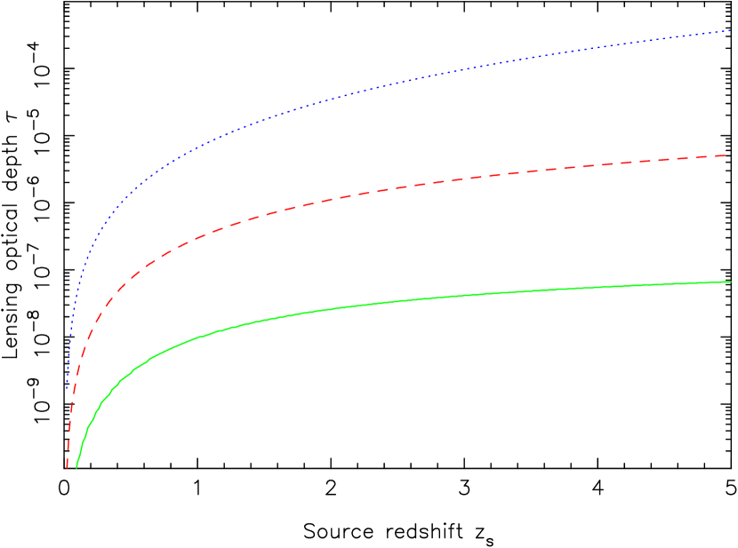
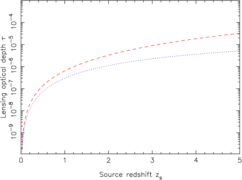
Figure 1: The optical depth $\tau$ as a function of source redshift. Left: with the angular resolution $\theta$ fixed at $0\aas@@fstack{\prime\prime}14$, we plot $\tau(z_{\rm s})$ for values of $G\mu/c^{2}=10^{-6}$ (dotted), $10^{-7}$ (dashed) and $5\times 10^{-8}$ (solid). Right: with $G\mu/c^{2}$ fixed at $10^{-7}$, we plot $\tau(z_{\rm s})$ for values of $\theta=0\aas@@fstack{\prime\prime}028$ (dashed), and $0\aas@@fstack{\prime\prime}14$ (dotted). The optical depth for image separations of 0.7 arcsec is negligible and does not appear on this plot.

The assumption behind equation (2) is that the overlaps given by the intersections of the long string projections on the sky are negligible with respect to the total cross-section. We now show that this is a reasonable assumption. Let us suppose we have $n$ such intersections; then the cross-section due to string intersections must be smaller than $\sim n(8\pi G\mu/c^{2})^{2}$. This is true if we require this quantity to be much smaller than $\sigma$, or that $\tau\gg 16\pi n(G\mu/c^{2})^{2}$. From Figure 1 we can see that for a realistic source redshift values ($z_{\rm s}>0.5$), the optical depth $\tau$ is of the order of $G\mu/c^{2}$. Therefore the requirement is $n\ll\left(G\mu/c^{2}\right)^{-1}$.

Recalling that the range of observation is well inside the Hubble horizon and the fact that only a few dozen long strings per Hubble volume are expected (see, e.g., Polchinski, 2004), the only way to have $n\sim 10^{6}$ or bigger is through overlap of the cross-section of a string with itself. Furthermore, once inside the horizon, the long strings tend to straighten through gravitational waves emission and loop breaking (Polchinski & Rocha, 2007). As a consequence, one do not expect a large amount of overlap for the range of redshift into consideration.

3 Expected number of observed string lensing events

The expected number of lensing events for a given experiment is the product $\Omega_{\rm s}\,N(G\mu/c^{2},\theta),$ where $\Omega_{\rm s}$ is the solid angle subtended by the survey in square degrees, and $N(G\mu/c^{2},\theta)$ is the expected number density of lensing events (in units of deg^-2). $N$ in turn is given by the integral of the optical depth over the source redshift distribution $\frac{dN_{\rm s}}{dz_{\rm s}}$, which, purely for concreteness, we take to be a Gaussian peaked at redshift $z_{\rm s}=1.5$ with width 0.4 normalized to 100 galaxies per square arcmin, appropriate for optical surveys reaching a limiting magnitude $I\sim 26$ mag (e.g. Benítez et al., 2004). This is a conservative limit for space based surveys, which can reach significantly higher density of (unresolved) galaxies. In any case, this normalization factor is degenerate with the area of a survey, and therefore one can easily generalize our results, trading area for number of background galaxies.

$$N(G\mu/c^{2},\theta)=3.6\times 10^{5}\int_{0}^{\infty}e^{-\frac{1}{2}\left(\frac{z_{\rm s}-1.5}{0.4}\right)^{2}}\tau(z_{\rm s},\theta,G\mu/c^{2})\,dz_{\rm s}.$$ (8)

Figure 2 gives $N(G\mu/c^{2},\theta)$ as a function of $\theta$ for fixed values of $G\mu/c^{2}=10^{-6},10^{-7}$ and $5\times 10^{-8}$, assuming a survey depth equivalent to recovering all 100 galaxies per square arcmin. In practice this may not be possible at the lowest angular resolution due to beam dilution, but as the steepness of Figure 2 implies, it is the angular resolution of the individual lens image pairs that is critical to the detection of the lensing events. In the next section we discuss the observational complications associated with detecting lensing by cosmic strings in practice.

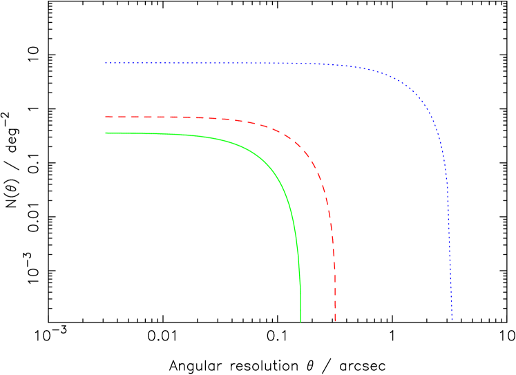
Figure 2: Predicted number density of lensing events $N$ per square degree as a function of the instrument angular resolution $\theta$/arcsec, for the fixed values of $G\mu/c^{2}=10^{-6}$ (dashed), $10^{-7}$ (dotted) and $5\times 10^{-8}$ (solid).

4 Observational Issues

We now turn briefly to the issue of practical lens system detectability. For a given string tension, and so image separation, the maximal detectability will be achieved with the sources as compact as possible, allowing them to be individually detected and flagged at the object catalogue level. However, if the angular resolution is such that the sources are well-resolved, then the possibility of detecting the lensing effect using sharp edge-detection algorithms is opened up. If the sources are resolved, morphological and colour information can be used to verify the cosmic string lensing hypothesis.

This somewhat idealistic case is altered if the string is moving relativistically, if the string is not straight on the length scale of the image separation in the plane of the string, or if the image is “cut” by the string so that one image is of only part of its source. The detection of strings may also be affected by the imaging survey “footprint” – thus far we have effectively assumed that the sources are observed one by one. We briefly discuss these possibilities in the rest of this section.

4.1 Relativistic strings

The relativistic movement of a string can significantly alter its lensing image separation and cause an apparent redshift between the two images (Vilenkin, 1986; Shlaer & Tye, 2005). Both effects arise from Lorentz-transforming from the frame of the string, in which the lensing occurs, into the frame of the observer and source. A string with a velocity component parallel to the line of sight $v_{\parallel}$ will have cross-section modified via

$$d\beta_{1}^{\prime}=\frac{\gamma d\beta_{1}}{(1-v_{\parallel}/c)},$$ (9)

which tends to infinity for highly relativistic strings! A full statistical treatment of the optical depth due to a network of fast-moving strings is beyond the scope of this paper, but the above considerations remind us of two things: first, that moving strings may be detectable by their lensing effects as well, and second that any bound on $G\mu/c^{2}$ is dependent on the assumptions of the string network kinematics. In subsequent sections we assume the non-relativistic limit, but note that current estimates based on numerical simulations give $(v/c)^{2}\sim 0.35$ (i.e. $(v_{\parallel}/c)^{2}\sim 0.2$ and $\gamma\sim 1.5$) at the present time (Polchinski, 2007), suggesting that our cross-sections are rather conservative. In any case, relativistic corrections will have to be taken into account in future studies in order to derive a precise limit for a specific survey.

A relativistically moving string with significant velocity in the plane of the sky ($v_{\perp}$) will also produce a redshift between the two sources given by

$$\Delta z=\frac{\gamma v_{\perp}d\beta_{1}}{c},$$ (10)

where $d\beta_{1}$ is measured in radians. This redshift perturbation would cause an apparent colour difference between the two images, warning us against the use of overly-restrictive cuts when filtering catalogues. However, unless the string is highly relativistic this redshift will be too small to be the dominant uncertainty in the relative image colour.

Bends in the string on the scale of the source size, and the “cutting” of sources whose image cross the line of the string, produce geometrical and even brightness distortions. The presence of many string lensing events in a small region of space is really the robust signature of the phenomenon (Huterer & Vachaspati, 2003; Oguri & Takahashi, 2005), but quantifying the identifiability of complex lensing events with detailed image simulations is possible. We describe an initial foray into this matter in the next subsection.

4.2 Practical image pair detection

The lensing signal we are looking for is an overdensity of close pairs of (resolved) galaxy images, aligned such that a string could pass through each one. There are three possible types of false positive for the individual candidate lens systems: physical close galaxy pairs, line of sight projections, and non-string gravitational lenses. The latter do not concern us for three reasons. First, the characteristic patterns of curved and distorted images in conventional galaxy-galaxy strong lenses (see e.g.  Bolton et al., 2006; Moustakas et al., 2007, for examples) are quite different from the translated and truncated images expected for a string lens (see e.g.  Sazhin et al., 2007, for examples). Second, in optical images of galaxy-galaxy strong lenses the lens galaxies are usually brighter than the images of the source, confirming the nature of the lens. Third, at a mean density of $\sim 10$ per square degree (Marshall et al., 2005), ordinary galaxy-scale strong lenses are sufficiently rare that one does not expect to find more than one in a field of view of a few square arcminutes (although see Fassnacht et al., 2006, for a notable counter-example).

The first two types of false positive – projected and physical close pairs of galaxies – can be rejected using high quality follow-up data (as in the case of CSL-1, Sazhin et al., 2007). Alternatively, during a survey they can be dealt with statistically via the observed galaxy two-point angular correlation function, a topic of active research by our group (Morganson et al., in preparation). In simulated HST F606W-band images with limiting magnitude 28 (comparable to the GOODS survey, for example, and assumed to contain background sources at a number density of 240 arcmin^-2), we find (on average) 4 faint galaxy pairs separated by $0\aas@@fstack{\prime\prime}5$ in a 1 arcsec by 5 arcmin image strip. We can compare this result to images that have been lensed by simulated strings. For illustration we consider a fiducial non-relativistic string of tension $G\mu/c^{2}=1.2\times 10^{-7}$ at $z_{\rm d}=0.5$ lying in the plane of the sky, and a population of compact, faint sources at $z_{\rm s}=1.5$. This set-up leads to a convenient source plane cross-section of width $d\beta_{1}=0\aas@@fstack{\prime\prime}5$. We generated mock background scenes, and then overlaid the string and recomputed the surface brightness where lensing occurs, then convolved the images with a mock HST PSF (FWHM $\approx 0\aas@@fstack{\prime\prime}14$) and added background and source Poisson noise consistent with the counts expected in an HST image of limiting magnitude 28.

In these simulated images we are able to detect an average of 14 faint galaxy pairs separated by by $0\aas@@fstack{\prime\prime}5$ in the same 1 arcsec by 5 arcmin strip (including 10 that are multiple images caused by the string). This number is consistent with that calculated by Sazhin et al. (2007). This simple observation of extra pairs is robust to moderate changes in color, magnitude and morphology caused by non-ideal strings, and would, in principle, require only one deep HST image in the right patch of sky – the simulated detection described above has a significance of more than 3-sigma. Moreover, the condition that the image pairs be aligned perpendicular to the putative string, and the requirement that all background objects be lensed if they are positioned behind the string, will allow the rejection of the majority of false positives.

4.3 Survey geometry

The optical depth is most relevant to a source-oriented survey, where all the sources in the sky are observed. The deduced lens number density calculated above is therefore an average event rate. The usual cosmological assumptions of isotropy and homogeneity do not necessarily apply to cosmic string lensing events. The possibility of having only a few long strings is favored by most models: the area around these strings could contain many detectable lensing events while the remaining (vast) expanse of sky would contain none. In practice, observing costs limit us to imaging surveys of a fixed area of the sky, which will include blank sky as well as sources and will be composed of some number of finite contiguous fields. The survey geometry is therefore rather important when the survey area is small, as we now show with a simple geometrical example.

Let us assume that we have a survey of total solid angle $A$ which is composed of a number of randomly distributed square fields each of side $2r$ radians, and area $a=4r^{2}$ steradians. Let us also assume that we have a single straight string of angular length $L$ which will be detected if it is within $r$ of the center of one of our fields. The probability any given field will detect our string is roughly the fraction of sky that is within $r$ of the string:

$$P_{\rm field} =\frac{1}{4\pi}\int_{-r}^{r}\int_{-r}^{L+r}\cos{\theta_{1}}d\theta_{1}d\theta_{2}$$

$$=\frac{2(L+2r)\sin r}{4\pi}\approx\frac{L\sqrt{a}}{4\pi}.$$ (11)

The probability of the survey containing a string in at least one of the $N=A/a$ fields is then

$$P_{\rm survey} =1-(1-P_{\rm field})^{N}$$

$$\approx 1-{\rm e}^{-\frac{NL\sqrt{a}}{4\pi}}$$

$$\approx 1-{\rm e}^{-\frac{L\sqrt{NA}}{41250{\rm deg}^{2}}}$$ (12)

This holds providing our many strings have cumulative length $L$ sufficiently long that the individual strings are much longer than $\sqrt{a}$, so that their overlap region is not large (Section 2). Also, it is clear that the random distribution of the fields is an important assumption in this simple calculation. Non-randomly chosen fields would have to be treated with more care.

As a practical example, we note that our assumption that $\rho_{\rm str}=60\rho_{\rm m}G\mu/c^{2}$ is equivalent to having 2250 degrees of string at $z<0.5$, independent of the string tension (recalling that simulations of string interactions indicate that the actual string density is within a factor two of this estimate). The independence arises because the string density is proportional to the tension, while the string length is just proportional to the density divided by the tension.

Assuming this string density then, a 5 square-degree survey divided into 1800 randomly-distributed small fields (each of e.g. $10$ arcmin², approximately the field of view of the Advanced Camera for Surveys aboard the Hubble Space Telescope) will contain a string with more than 99% probability. However, with the same density and survey area but a contiguous survey geometry, the string would only fall in the survey region with 11% probability, and we would not be able to confidently place a limit on $\mu$.

Conversely, surveys of more than a few square degrees will reliably contain strings even without many divisions. We find that, in order to achieve a 95% probability of including a long string, surveys of area 0.5, 5, and 1000 square degrees must be divided into 6000 fields, 600 fields and 3 fields respectively (assuming the string density of section 2). Total survey areas greater than these are large enough to be guaranteed a string crossing, regardless of their geometry. For the rest of this paper we assume that the imaging survey in question is composed of randomly distributed fields that are sufficiently small to make the average lensing event rate given by the theoretical optical depth appropriate for interpreting the observations.

5 Bounds on $G\mu/c^{2}$

If a single detection of string lensing was made, then the optical depth would not be zero, and a lower bound could be put on the string tension $G\mu/c^{2}$. This bound would be given by the angular resolution of the experiment, as described at the end of section 2. It is a lower bound since the maximum image separation occurs when the string is right in front of the observer – moving the string to higher redshift would require a larger tension to keep the image separation as large as observed. If somehow the string redshift can be constrained, statistically or via the presence of foreground non-lensed objects, then the image separation provides direct measurement of the string tension.

On the other hand, if nothing is observed we cannot state that the upper bound on $G\mu/c^{2}$ is given by this “angular resolution bound” argument. We expect the upper bound to be bigger than $\frac{\theta}{16}$, with the exact amount by which it is bigger dependent on the observed sky area $\Omega_{\rm s}$, and the source density distribution $\frac{dN_{\rm s}}{dz_{\rm s}}.$ Treating string lensing events as rare, and so using the Poisson distribution for the probability of their occurrence given the predicted mean rate (previous section), then if no string lensing detections are made, we can state at $95\%$ confidence that the upper bound on $G\mu/c^{2}$ is given by the root of $N(G\mu/c^{2},\theta)=\frac{2.996}{\Omega_{s}}$ (Gehrels, 1986).

Angular		Survey area (deg2)
Resolution	$0.5$	5	1000	20,000
0$\aas@@fstack{\prime\prime}028$	$<8.4\times 10^{-7}$	$<9.1\times 10^{-8}$	$<1.1\times 10^{-8}$	$<9.0\times 10^{-9}$
0$\aas@@fstack{\prime\prime}14$	$<8.6\times 10^{-7}$	$<1.5\times 10^{-7}$	$<4.7\times 10^{-8}$	$<4.3\times 10^{-8}$
0$\aas@@fstack{\prime\prime}7$	$<1.1\times 10^{-6}$	$<4.0\times 10^{-7}$	$<2.2\times 10^{-7}$	$<2.1\times 10^{-7}$

Table 1: Inferred upper limits (95%) on the string tension corresponding to no detection, for a variety of combinations of instrumental resolution and survey area.

We now place our simple theoretical calculation in observational context, building on the discussion in section 4. We anticipate requiring surveys covering large areas of sky, and observing high surface densities of faint galaxies at high angular resolution, but aim to show the link between what is possible now and what may be possible in the future, wide-field era. We investigate three representative angular resolutions, typical of ground-based optical imaging ($0\aas@@fstack{\prime\prime}7$), of space-based optical/infra-red imaging ($0\aas@@fstack{\prime\prime}14$), and of planned radio surveys ($0\aas@@fstack{\prime\prime}028$). (This last resolution may also be achievable with next generation adaptive optics on large optical telescopes, although the area surveyed will be necessarily smaller.) We have purposely tried to be conservative in these angular resolutions. For simplicity we do not account for the different survey depths. In most cases the number of background sources will be irrelevant beyond some threshold, as will be the area of the surveys, since the factor dominating the sensitivity is the angular resolution. Figure 3 shows the expected number density of string lensing events, as a function of $G\mu/c^{2}$, for our three fiducial survey resolutions.

Table 1 shows upper limits on $G\mu/c^{2}$ in the event of a null survey result for surveys of various solid angles. square degrees. The first two choices of sky area (0.5 and 5 square degrees) represent high resolution surveys within current capabilities (e.g., the HST-ACS archive, Marshall et al. 2007, in prep). The larger survey areas, 1000 and 20000, square degrees, represent reasonable expectations for the next generation of space and ground based surveys, respectively (see e.g. Aldering et al., 2004; Tyson et al., 2006).

Let us illustrate this table a little. For example, for a fixed resolution of $\theta=0\aas@@fstack{\prime\prime}14$, choosing $\Omega_{\rm s}=5$ square degrees gives $G\mu/c^{2}\leq 1.5\times 10^{-7}$. This limit is about a factor of two lower than the most recent $95\%$ confidence bound from studies of the cosmic microwave background (Pogosian et al., 2006; Seljak & Slosar, 2006; Jeong & Smoot, 2007), and is competitive with the pulsar timing studies by virtue of having different model dependencies (the reader is referred to Polchinski (2007) for a critical review of current observational bounds on $G\mu/c^{2}$).

Note that, because of the steep shape of the curve near this value (Figure 3), observing a larger area of sky without (long) string lensing observations would not give a proportionate decrease in the bound on$~{}G\mu/c^{2}$. Even though this may appear surprising at first, this is a simple consequence of the fact that the main limitation in fixing the bound comes from the angular resolution.

In other words, for any given resolution there is a maximum area that is worth exploring for strings, the exact value of which will depend on the survey geometry, the string correlation length and the image depth (i.e. on the number of available background source galaxies). For example, at ground-based optical image resolution ($0\aas@@fstack{\prime\prime}7$), a survey of $\sim 30$ square degrees is sufficient to reach saturation – and even then the resulting upper limit on the string tension is above that available from a few square degrees of space-based resolution optical imaging. At the highest resolution considered here, this maximum area is correspondingly higher; however, we can see that the difference between 1000 square degrees and half the sky is small (a mere 20% improvement in the bound on $G\mu/c^{2}$). To make progress then, one needs better resolution first, and then more area.

This conclusion has two practical consequences. On the one hand, data already exist that can probe the $G\mu/c^{2}\sim 10^{-7}$ regime, with a suitably robust algorithm (Morganson et al., in preparation). On the other hand, we have not yet reached the maximum useful area for space-based optical string lens surveys: the turnover in Figure 3 for $0\aas@@fstack{\prime\prime}14$ resolution is at a few hundred square degrees. Moving to even higher resolution at the same scale of survey will result in a gain of a further factor of 5 or so, ultimately providing sensitivity to string tensions of $G\mu/c^{2}\sim 10^{-8}$.

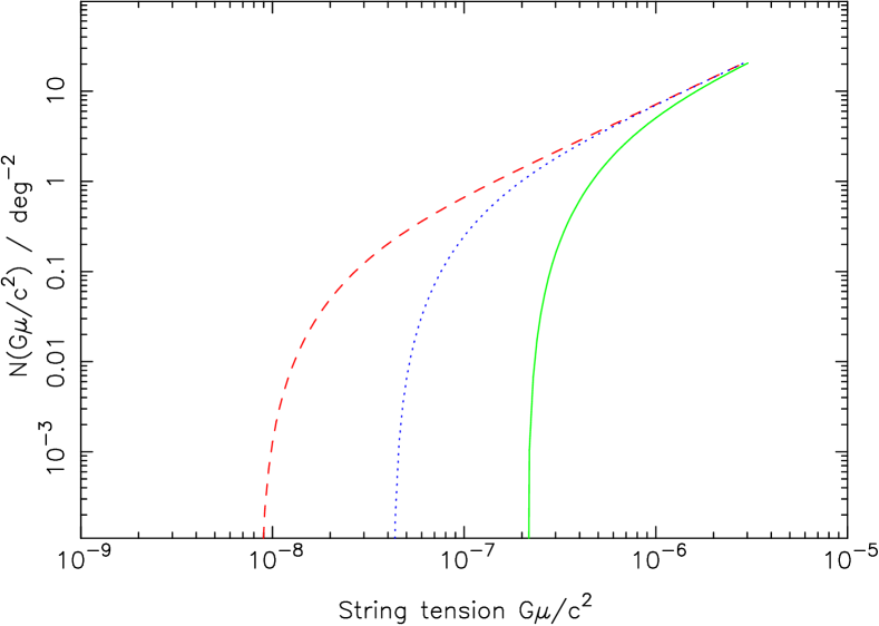
Figure 3: The predicted number density of string lensing events $N$ per square degree as a function of $G\mu/c^{2}$, for three values of the angular resolution $\theta=0\aas@@fstack{\prime\prime}028$ (dashed), $0\aas@@fstack{\prime\prime}14$ (dotted) and $0\aas@@fstack{\prime\prime}7$ (solid).

6 Conclusions

We have used a robust prediction of theoretical work on cosmic string networks to predict, in a straightforward way, the expected number of strong gravitational lensing events visible in astronomical imaging surveys of varying angular resolution and sky coverage. From our simple analysis we draw the following conclusions:

1. Present-day high-resolution imaging surveys are capable of probing the putative cosmic string tension parameter to a factor of two lower than the current CMB limit, making lensing both competitive with, and complementary to, the pulsar timing methods. As has been noted before, in the event of a detection, gravitational lensing would provide a direct measurement of the tension, and perhaps the velocity, of this string.

2. The main practical considerations in detecting string lensing events are two-fold: firstly, the expected faint pairs of images must first be carefully deblended and then understood in the context of neighbouring events; secondly, the survey geometry should be such that the fields are large enough to contain the characteristic multiple neighbouring events, but sparsely distributed to ensure that the global, not local, lensing rate is being probed.

3. The upper bound on the tension, from the failure to detect a single string lensing event in a given survey, is principally determined by the available angular resolution. Relatively little is gained from studying an area of sky greater than some critical value: for typical ground-based optical image resolution, this critical survey size is a few tens of square degrees. Likewise, string tensions of $G\mu/c^{2}\sim 10^{-8}$ should be able to be investigated in future surveys with image resolutions of 10-100 milliarcsec covering a few hundred square degrees.

References

- Agol et al. (2006) Agol, E., Hogan, C. J., & Plotkin, R. M. 2006, Phys.Rev.D, 73, 087302
- Aldering et al. (2004) Aldering, G., et al. 2004, arXiv:astro-ph/0405232
- Benítez et al. (2004) Benítez, N., Ford, H., Bouwens, R., Menanteau, F., Blakeslee, J., Gronwall, C., Illingworth, G., Meurer, G., Broadhurst, T. J., Clampin, M., Franx, M., Hartig, G. F., Magee, D., Sirianni, M., Ardila, D. R., Bartko, F., Brown, R. A., Burrows, C. J., Cheng, E. S., Cross, N. J. G., Feldman, P. D., Golimowski, D. A., Infante, L., Kimble, R. A., Krist, J. E., Lesser, M. P., Levay, Z., Martel, A. R., Miley, G. K., Postman, M., Rosati, P., Sparks, W. B., Tran, H. D., Tsvetanov, Z. I., White, R. L., & Zheng, W. 2004, ApJS, 150, 1
- Bolton et al. (2006) Bolton, A. S., Burles, S., Koopmans, L. V. E., Treu, T., & Moustakas, L. A. 2006, ApJ, 638, 703
- Damour & Vilenkin (2005) Damour, T., & Vilenkin, A. 2005, Phys.Rev.D, 71, 063510
- Davis & Kibble (2005) Davis, A.-C., & Kibble, T. 2005, Contemporary Physics, 46, 313
- Fassnacht et al. (2006) Fassnacht, C. D., McKean, J. P., Koopmans, L. V. E., Treu, T., Blandford, R. D., Auger, M. W., Jeltema, T. E., Lubin, L. M., Margoniner, V. E., & Wittman, D. 2006, ApJ, 651, 667
- Gehrels (1986) Gehrels, N. 1986, ApJ, 303, 336
- Huterer & Vachaspati (2003) Huterer, D., & Vachaspati, T. 2003, Phys.Rev.D, 68, 041301
- Jeong & Smoot (2007) Jeong, E., & Smoot, G. F. 2007, ApJ, 661, L1
- Kaspi et al. (1994) Kaspi, V. M., Taylor, J. H., & Ryba, M. F. 1994, ApJ, 428, 713
- Kibble (1976) Kibble, T. W. B. 1976, J. Phys. A: Math. Gen. 9, 1387
- Lo & Wright (2005) Lo, A. S., & Wright, E. L. 2005, arXiv:astro-ph/0503120
- Mack et al. (2007) Mack, K. J., Wesley, D. H., & King, L. J. 2007, arXiv:astro-ph/0702648
- Marshall et al. (2005) Marshall, P., Blandford, R., & Sako, M. 2005, New Astronomy Review, 49, 387
- Moustakas et al. (2007) Moustakas, L. A., Marshall, P., Newman, J. A., Coil, A. L., Cooper, M. C., Davis, M., Fassnacht, C. D., Guhathakurta, P., Hopkins, A., Koekemoer, A., Konidaris, N. P., Lotz, J. M., & Willmer, C. N. A. 2007, ApJ, 660, L31
- Oguri & Takahashi (2005) Oguri, M., & Takahashi, K. 2005, Phys.Rev.D, 72, 085013
- Pogosian et al. (2006) Pogosian, L., Wasserman, I., & Wyman, M. 2006, arXiv:astro-ph/0604141
- Polchinski (2004) Polchinski, J. 2004, in Lectures presented at the 2004 Cargese Summer School
- Polchinski (2007) Polchinski, J. 2007, in Proceedings of the Eleventh Marcel Grossmann Meeting on General Relativity, ed. R. J. H. Kleinert & R. Ruffini (World Scientific: Singapore)
- Polchinski & Rocha (2007) Polchinski, J., & Rocha, J. V. 2007, Phys.Rev.D, 75, 123503
- Sazhin et al. (2007) Sazhin, M. V., Khovanskaya, O. S., Capaccioli, M., Longo, G., Paolillo, M., Covone, G., Grogin, N. A., & Schreier, E. J. 2007, MNRAS, 376, 1731
- Schneider (2006) Schneider, P. 2006, in Gravitational Lensing: Strong, Weak & Micro, ed. G. Meylan, P. Jetzer, & P. North, Lecture Notes of the 33rd Saas-Fee Advanced Course (Springer-Verlag: Berlin)
- Seljak & Slosar (2006) Seljak, U., & Slosar, A. 2006, Phys.Rev.D, 74, 063523
- Shlaer & Tye (2005) Shlaer, B., & Tye, S.-H. H. 2005, Phys.Rev.D, 72, 043532
- Tyson et al. (2006) Tyson, J. A., et al. 2006, http://www.lsst.org/Science/docs
- Vilenkin (1984) Vilenkin, A. 1984, ApJ, 282, L51
- Vilenkin (1986) —. 1986, Nature, 322, 613