Size effects in the exchange coupling between two electrons in quantum wire quantum dots

Abstract

We theoretically investigate the properties of a two-electron system confined in the three-dimensional potential of coupled quantum dots formed in a quantum wire. For this purpose, we implement a variational Heitler-London method that minimize the system energies with respect to variational parameters in electron trial wavefunctions. We find that tunneling and exchange couplings exponentially decay with increasing inter-dot distance and inter-dot barrier height. In the quasi-one-dimensional limit achieved by reducing the wire diameter, we find that the overlap between the dots decreases, which results in a drop of the exchange coupling. We also discuss the validity of our variational Heitler-London method with respect to the model potential parameters, and compare our results with available experimental data to find good agreement between the two approaches.

I Introduction

Very recently, the exploration of new hardware schemes at the frontier of solid state quantum computing has unveiled a new approach to fabricate coupled quantum dots (QDs) with controlling gate grid adjacent to an InAs quantum wire (QW).SamGroup In these device structures, electrons are laterally confined (i.e., perpendicular to the axial direction of the wire) by the wire external surfaces (wire diameters are tens or even a few nanometers),Bjork and longitudinally confined in the wire axial direction by the electrostatic potential barriers created by the local controlling gates. The local gate width and separation range from $\sim 10$ to $\sim 100$ nm, which results in small effective dot sizes and inter-dot separations, so that size quantization effects and exchange coupling between the QDs are expected to be significantly larger than that in the two dimensional electron gas (2DEG) based semiconductor QDs.Fasth In quantum wire quantum dot (QWQD) systems, the distance between the controlling gates and the QD region ($\sim 25$ nm)SamGroup is smaller than that in 2DEG-based QDs ($\sim 100$ nm),Petta leading to better electrostatic control of the charge (spin) states in the QDs. Furthermore, QWQD structures offer linear scalability (i.e., with the linear grid of the controlling gates) instead of the 2D scalability resulting from top or side gate patterning in 2DEG-based QDs.SamGroup

In laterally coupled 2DEG-based QDs, electron coupling occurs between the two QDs in the same plane as the 2DEG, and carrier confinement is much stronger in the perpendicular direction.Petta ; Elzerman ; Hatano In vertically coupled 2DEG-based QDs, carrier confinement is weaker in the 2DEG plane than that in the coupling (vertical) direction (see e.g., Refs. Pi, and Bellucci, and references therein). The electron confinement and coupling defined in the fabrication processes of coupled QWQDs considerably deviate from those achieved in the 2DEG-based coupled QDs: the electrons are strongly confined in the plane perpendicular to the axial direction of the wire because of the small wire diameter, while quantum mechanical coupling is achieved between two quantum wells with relatively weaker confinement, because of the controlling gate spacing and biases.

While a wealth of literature has been dedicated to the theoretical study of 2DEG-based coupled QDs,Burkard1 ; Dmm1 ; Hu ; Harju ; Szafran ; Dybalski ; Zhang1 ; Zhang2 ; Stopa less attention is paid to the QWQD systems. Among all investigated approaches, the Heitler-London (HL) technique is relatively simple in its conceptual methodology to extract the exchange coupling between coupled QDs:Burkard1 ; Hu its validity has been discussed for systems of various dimensions,Calderon and efforts have been pursued to improve the energy calculation by integrating variational parameters in the HL method.Burkard2 ; Koiller

In this paper, we compute the electronic structure of coupled QWQDs containing two electrons with a variational Heitler-London (VHL) method. We first construct a three-dimensional (3D) model confinement potential for the QWQDs and introduce three variational parameters in the HL wavefunctions that account for the specific 3D confinement profile. We then numerically minimize the QWQD energies with respect to these parameters, and obtain the quantum mechanical and exchange couplings between the two electrons, as well as the addition energy of the second electron in the dot. In our analysis, special emphasis is placed on the geometric effects in the coupled QWQDs. We discuss the limitations of our VHL method but indicate its improvement over the conventional HL method. We finally compare our results with the available experimental data.

II model and method

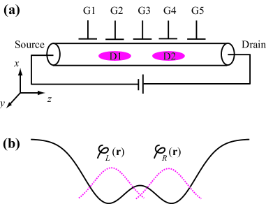
Figure 1: (color online) (a) Schematic of coupled QDs $D1$ and $D2$ formed in a quantum wire. Gates $G1$ and $G5$ define the outer barriers of the two QDs; $G3$ controls the inter-dot coupling; $G2$ and $G4$ are plungers tuning the confinement in each QD. Charging current flows along the wire from source to drain. (b) Schematic of the confinement potential of the coupled QDs along the $z$ (wire axial) direction. $\varphi_{L}({\bf r})$ and $\varphi_{R}({\bf r})$ denote the localized $s$ states in the left and right QDs, respectively.

Figure 1(a) shows a schematic of coupled QDs $D1$ and $D2$ formed in a single quantum wire: gates $G1$ and $G5$ define the outer barriers of the QDs, $G3$ controls the inter-dot coupling, and $G2$ and $G4$ are used as plunger gates for fine tuning of the potential in each QD. The charging current flows from source to drain along the wire. The material under consideration is InAs, for which we use the electron effective mass $m=0.023m_{0}$ (Ref. AEHanson, ) and dielectric constant $\epsilon=14.6$. Hence, the effective Bohr radius $r_{0}=\hbar^{2}\epsilon/me^{2}=33.6$ nm and effective Rydberg constant $Ry=me^{4}/2\epsilon^{2}\hbar^{2}=1.468$ meV. We assume a parabolic confinement potential in the $xy$-plane $V({\bm{\rho}})={m}\Omega_{\rho}^{2}{\bm{\rho}}^{2}/2$, wherein we take $\Omega_{\rho}=\hbar/m(D/2)^{2}$, and $D$ is the nominal value of the wire diameter. In the $z$-direction (along which the QDs are coupled), the confinement potential is modeled by a linear combination of three Gaussians:

$$V(z) = -V_{0}\left\{\exp\left[-\frac{(z-d)^{2}}{l_{z}^{2}}\right]+\exp\left[-\frac{(z+d)^{2}}{l_{z}^{2}}\right]\right\}$$ (1)

$$+V_{b}\exp\left(-\frac{z^{2}}{l_{bz}^{2}}\right),$$

where $V_{0}$ gives the depth of two Gaussian wells describing the confinement of the two individual QDs (we fix $V_{0}=20$ meV), $V_{b}$ controls the barrier height between the two wells ($V_{b}=0$ except otherwise specified), $l_{z}$ is the radius of each QD, $2d$ is the nominal separation between the two QDs, and $l_{bz}$ denotes the radius of the central barrier. A schematic of $V(z)$ is shown in Fig. 1(b) by the solid line. The two electrons in the coupled QDs are described by the following Hamiltonian:

$$\hat{H}=\hat{H}_{orb}+\hat{H}_{Z},$$ (2)

$$\hat{H}_{orb}=\hat{h}_{1}+\hat{h}_{2}+\frac{e^{2}}{\epsilon\left|{\bf r_{1}}-{\bf r_{2}}\right|},$$ (3)

$$\hat{h}_{i}=\frac{1}{2m}\left({\bf p_{\rho}}_{i}+\frac{e}{c}{\bf A}_{i}\right)^{2}+V({\bm{\rho}}_{i})+\frac{1}{2m}{{\bf p}_{z}}_{i}^{2}+V(z_{i}),$$ (4)

$$\hat{H}_{Z}=g\mu_{B}\sum_{i}{\bf B}\cdot{\bf S}_{i}.$$ (5)

Note that we separate the motion of the electron in the $xy$-plane and in the $z$-direction in the single-particle Hamiltonian $\hat{h}_{i}$. In this work, we only consider magnetic fields applied in the $z$-direction for which ${\bf A}=\left(-yB{\hat{x}}+xB{\hat{y}}\right)/2$. Such a magnetic field effectively enhances the confinement of the in-plane ($xy$-plane) ground state while preserving its cylindrical symmetry.

In order to obtain the system energies, we use the following trial wavefunctions:

$$\chi_{\pm}({\bf r})=\frac{\varphi_{L}({\bf r})\pm\varphi_{R}({\bf r})}{\sqrt{2(1\pm S)}},$$ (6)

$$\Psi_{\pm}\left({\bf r}_{1},{\bf r}_{2}\right)=\frac{\varphi_{L}({\bf r}_{1})\varphi_{R}({\bf r}_{2})\pm\varphi_{L}({\bf r}_{2})\varphi_{R}({\bf r}_{1})}{\sqrt{2(1{\pm}S^{2})}}.$$ (7)

In above, $\chi_{+}$, $\chi_{-}$, $\Psi_{+}$ and $\Psi_{-}$ denote the single-particle ground and first excited states, two-electron singlet and triplet states, respectively. $S=<\varphi_{L}|\varphi_{R}>$ is the overlap between $s$ orbitals $\varphi_{L}({\bf r})$ and $\varphi_{R}({\bf r})$ localized in the left and right QDs, respectively, and their specific expressions are

$$\varphi_{L/R}({\bf r}) = \left(\frac{{m}\omega_{\rho}}{\pi\hbar}\right)^{\frac{1}{2}}\exp\left[-\frac{{m}\omega_{\rho}}{2\hbar}(x^{2}+y^{2})\right]$$ (8)

$$\times\left(\frac{{m}\omega_{z}}{\pi\hbar}\right)^{\frac{1}{4}}\exp\left[-\frac{{m}\omega_{z}}{2\hbar}(z\pm a)^{2}\right].$$

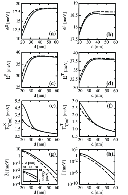
Figure 2: (a) Single-particle ground state energy, (b) single-particle first excited state energy, (c) two-electron singlet state energy, (d) two-electron triplet state energy, (e) Coulomb energy in the singlet state, (f) Coulomb energy in the triplet state, (g) tunneling coupling $2t$, and (h) exchange interaction as a function of the half inter-dot separation $d$ for $l_{z}=30$ nm and $D=20$ nm. The inset in (g) shows $2t$ in the zoom-in region $20<d<30$ nm. On each panel, the solid (dashed) line shows the VHL (HL) result.

Figure 1(b) shows the schematic of $\varphi_{L}({\bf r})$ and $\varphi_{R}({\bf r})$ in the $z$-direction by dashed lines on top of the potential. With the variational wavefunctions, we calculate the single-particle ground and first excited state energies $e^{0/1}=\left<\chi_{\pm}\left|\hat{h}\right|\chi_{\pm}\right>$, two-electron singlet and triplet state energies $E^{S/T}=\left<\Psi_{\pm}\left|\hat{H}_{orb}\right|\Psi_{\pm}\right>$. The detailed expressions of these matrix elements are given in the Appendix.

In our VHL approach, we use the effective in-plane confinement strength $\omega_{\rho}$, $z$-direction confinement strength $\omega_{z}$ and effective half inter-dot separation $a$ as variational parameters to minimize the system energies.footnote By fixing these variational parameters equal to their nominal values $\omega_{\rho}=\sqrt{\Omega_{\rho}^{2}+\omega_{c}^{2}}$ with $\omega_{c}=eB/mc$, $\omega_{z}=\Omega_{z}=\sqrt{2V_{0}/ml_{z}^{2}}$ and $a=d$, we recover the results from the conventional HL method. We calculate the Coulomb energies in the singlet and triplet states by

$$E_{Coul}^{S/T} = \left<\Psi_{\pm}\left|C\right|\Psi_{\pm}\right>$$ (9)

$$= \frac{1}{1\pm S^{2}}\left(\left<\varphi_{L}\varphi_{R}\left|C\right|\varphi_{L}\varphi_{R}\right>\right.$$

$$\pm\left.\left<\varphi_{L}\varphi_{R}\left|C\right|\varphi_{R}\varphi_{L}\right>\right),$$

where $C=e^{2}/\epsilon|{\bf r}_{1}-{\bf r}_{2}|$, and we have used the notation

$$\left<\varphi_{L}\varphi_{R}\left|C\right|\varphi_{L}\varphi_{R}\right>$$

$$=\left<\varphi_{L}({\bf r}_{1})\varphi_{R}({\bf r}_{2})\left|C\right|\varphi_{L}({\bf r}_{1})\varphi_{R}({\bf r}_{2})\right>,$$ (10)

$$\left<\varphi_{L}\varphi_{R}\left|C\right|\varphi_{R}\varphi_{L}\right>$$

$$=\left<\varphi_{L}({\bf r}_{1})\varphi_{R}({\bf r}_{2})\left|C\right|\varphi_{R}({\bf r}_{1})\varphi_{L}({\bf r}_{2})\right>.$$ (11)

The same notation has been used in expressing the matrix elements in the Appendix. Using both HL and VHL methods, we calculate the tunnel coupling $2t=e^{1}-e^{0}$ and the exchange coupling $J=E^{T}-E^{S}$. From the two electron wavefunctions, we compute the electron density as [$\varphi_{L/R}({\bf r})$ are real]

$$\rho^{S/T}({\bf r}_{1}) = 2\int\left|\Psi_{\pm}\left({\bf r}_{1},{\bf r}_{2}\right)\right|^{2}d{\bf r}_{2}$$ (12)

$$= \frac{1}{1\pm S^{2}}\left[\varphi_{L}^{2}({\bf r}_{1})+\varphi_{R}^{2}({\bf r}_{1})\right.$$

$$\pm\left.2S\varphi_{L}({\bf r}_{1})\varphi_{R}({\bf r}_{1})\right].$$

III results

In Fig. 2, we plot (a) the single-particle ground state energy $e^{0}$, (b) single-particle first excited state energy $e^{1}$, (c) two-electron singlet state energy $E^{S}$ and (d) two-electron triplet state energy $E^{T}$ as a function of the half inter-dot separation $d$ for $l_{z}=30$ nm and $D=20$ nm. The solid and dashed lines show the results obtained from VHL and HL methods, respectively, from which we see that VHL method indeed gives lower system energies than the HL method. Here, we note that each energy is minimized with respect to a set of its own variational parameters. We also note that the single-particle energies are positive simply because of the large energy contribution from the in-plane confinement: for $D=20$ nm, $\hbar\omega_{\rho}\approx 33$ meV and is changed by less than $1\%$ by varying $d$.

For $l_{z}=30$ nm and $d=20$ nm, the two Gaussian wells in Eq. (1) are strongly coupled. As a result, the $z$-direction potential has a single minimum at $z=0$, corresponding to a single QD. As $d$ increases, a potential barrier between the QDs starts to emerge (for $d>21.2$ nm). Meanwhile, the potential minimum is raised, and the $z$ confinement in each individual QD becomes stronger. The behavior of the single-particle energies is a result of these combined effects. For example, as $d$ increases from $20$ to $38$ nm, both $e^{0}$ and $e^{1}$ sharply increase due to the large increase of the potential minimum [Figs. 2(a) and (b)]. For $38<d<60$ nm, $e^{0}$ still slowly increases, while $e^{1}$ starts to decrease. Our analysis based on the variational parameters shows competing effects of the kinetic and potential energies in this region: for $e^{0}$, the kinetic energy increase dominates a slight drop of the potential energy, whereas for $e^{1}$, the potential energy increase is offset by the drop in the kinetic energy. For very large $d$, both $e^{0}$ and $e^{1}$ approach a constant value ($18.53$ meV), which corresponds to the limit of two decoupled quantum wells.

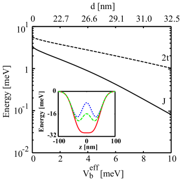
Figure 3: (color online) Main panel: Exchange coupling $J$ (solid curve) and tunnel coupling $2t$ (dashed curve) as a function of the effective barrier height $V_{b}^{eff}$. Values of half inter-dot separation $d$ corresponding to different $V_{b}^{eff}$ values are shown on the upper horizontal scale. Inset: $z$-direction potential profile at $V_{b}^{eff}$ values $0$ meV (red, solid), $5$ meV (green, dashed) and $10$ meV (blue, dotted). Corresponding $V_{b}$ values are $-14.71$ meV, $-1.16$ meV and $6.65$ meV, respectively. Values of other parameter are: $D=20$ nm, $d=l_{z}=30$ nm, and $l_{b}=30$ nm.

The behavior of $E^{S}$ and $E^{T}$ [Figs. 2(c) and (d)] resembles that of $e^{0}$ and $e^{1}$, albeit a drop for $d>41$ nm is observed for both quantities. The similarity implies that the single-particle energies are the dominant contributions to $E^{S}$ and $E^{T}$, whereas the decrease of Coulomb energy with increasing $d$ [Figs. 2 (e) and (f)] has a minor influence. It is seen that at fixed $d$, the Coulomb interaction is stronger in the singlet state, due to the larger overlap ($S$) in the two-electron wavefunction, which is a signature of the Pauli exclusion principle.

In Figs. 2 (g) and (h), we plot the tunnel coupling $2t$ and exchange coupling $J$ as a function of $d$, respectively, both of which exhibit exponential decay with increasing $d$ (strictly speaking, the decay is slightly slower than exponential). In these figures, the solid (dashed) line corresponds to the VHL (HL) result. A much larger decrease of $J$ ($\sim 10^{-8}$) than $2t$ ($\sim 10^{-4}$) as $d$ increases from $20$ to $60$ nm agrees qualitatively with the Hubbard model $J\propto(2t)^{2}/U_{H}$, assuming that the intra-dot Coulomb interaction $U_{H}$ retains the same order of magnitude as $d$ varies. Figs. 2 (g) and (h) show a large difference between the tunnel and exchange couplings obtained by using the HL and VHL methods, from which we notice that the HL method substantially underestimates the coupling between the two electrons,Sousa especially for large inter-dot separations. For example, at $d=60$ nm, the VHL result of $2t$ ($J$) is $\sim 10$ ($\sim 100$) times of the HL result.

The inset in Fig. 3 indicates that both the effective barrier height $V_{b}^{eff}$ (i.e., the energy difference between the minima of the potential and its value at $z=0$) and the distance between the two QDs (i.e., the distance between the two minima of the potential) become larger as $V_{b}$ is increased. Consequently, both $2t$ and $J$ exhibit nearly exponential decayHu with increasing $V_{b}^{eff}$ as shown in the main panel of Fig. 3, similar to the quasi-exponential drop of these two quantities with increasing QD separation $2d$ [cf. Figs. 2(g) and (h)]. Again, we observe that $J$ decays at a much faster rate than $2t$. In experimental QWQD devices, the effective barrier height between the two QDs can be tuned by varying the central gate bias,SamGroup and our analysis shows that the magnitude of the exchange coupling can be controlled by proper biasing the central gate as in 2DEG-based coupled QDs.Hu

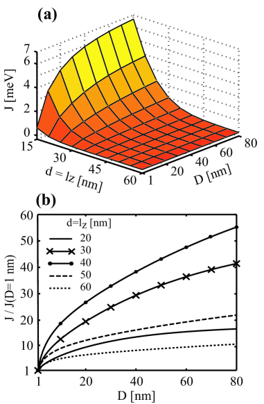
Figure 4: (color online) (a) Exchange coupling $J$ as a function of wire diameter $D$ and half separation between the QDs $d$, which is set equal to QD radius $l_{z}$ ($d=l_{z}$). (b) $J$ as a function of $D$ for different $d=l_{z}$ values (shown in the figure). The $J$ value on each curve is normalized to its value at $D=1$ nm. For $(d=l_{z})=20$, $30$, $40$, $50$, $60$ nm, $J(D=1\text{nm})=2.33\times 10^{-1}$, $2.47\times 10^{-2}$, $3.53\times 10^{-3}$, $1.37\times 10^{-3}$, $4.81\times 10^{-4}$ meV, respectively.

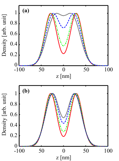
Figure 5: (color online) Electron density plot in the $z$-direction for (a) singlet and (b) triplet states at $d=l_{z}=30$ nm. In each figure, the density is plotted at $D=1$ nm (red, solid), $D=10$ nm (green, dashed-dotted), $D=40$ nm (blue, dashed) and $D=80$ nm (black, dotted). For each $D$, the density is normalized to its peak value.

Figure 4(a) displays the exchange coupling $J$ as a function of both the wire diameter $D$ and the half separation ($d$) between the two QDs. Here, we set $d=l_{z}$ noting that in experiments coupled QWQDs are defined on top of a linear gate grid with a particular periodicity,SamGroup which indicates that the effective QD size and inter-dot separation are approximately the same. For the confinement potential given by Eq. (1), this configuration leads to a constant effective barrier height of $5.68$ meV, independent of the value of $d=l_{z}$. The nominal confinement strength for a single Gaussian well ($V_{0}=20$ meV) with $l_{z}=15$ nm ($0.45r_{0}$) and $60$ nm ($1.78r_{0}$) is $\hbar\Omega_{z}=24.27$ and $6.07$ meV, respectively. For a wire diameter $D=1$ nm, the nominal confinement is $\hbar\Omega_{\rho}=1.33\times 10^{4}$ meV, which physically corresponds to the quasi-1D limit of the systems with aspect ratio $(\lambda_{\rho}/\lambda_{z}=\sqrt{\Omega_{z}/\Omega_{\rho}})<0.05$ for the investigated range of $d=l_{z}$ from $15$ to $60$ nm. In the opposite limit, where $D=80$ nm, $\hbar\Omega_{\rho}=2.07$ meV, the aspect ratio $\lambda_{\rho}/\lambda_{z}>1.71$. At fixed $D$, $J$ exhibits exponential decay with $d=l_{z}$ in Fig. 4(a), where it is also observed that $J$ decreases with decreasing $D$ at fixed $d=l_{z}$. This trend is shown explicitly in Fig. 4(b) for different $d=l_{z}$. For comparison, the data on each curve are normalized to the value of $J$ at $D=1$ nm. At fixed $d=l_{z}$, as $D$ is decreased from $80$ nm, $J$ decreases, and the decreasing rate becomes larger as $D$ approaches $1$ nm, which is the $quasi-1D$ limit. The faster dropping rate of $J$ near $D=1$ nm is due to $\Omega_{\rho}\propto 1/D^{2}$, and the influence of the variation of $\Omega_{\rho}$ on $J$ becomes stronger at smaller $D$ (through the Coulomb interaction). Here, we note that although the general trend of $J$ is to decrease as $D$ is made smaller, the decreasing rates are much larger for intermediate $d=l_{z}$ values than for small or large values.

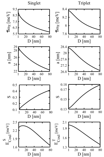
Figure 6: Variational parameters $\omega_{z}$ (shown as $\hbar\omega_{z}$), half separation $a$, the overlap $S$, and the Coulomb energies as a function of $D$ at $d=l_{z}=30$ nm. Left (right) panels are for the singlet (triplet) state.

These effects of the wire diameter variation on the exchange coupling are rather unexpected as they show that $J$ depends on the wire confinement perpendicular to the coupling direction. In fact, we find that the $D$ variation not only changes $\omega_{\rho}$, but also induces significant changes in $\omega_{z}$ and $a$, which minimize the singlet and triplet state energies. One can directly visualize such changes by inspecting the electron density variation with respect to the wire diameter. In Fig. 5, we plot the electron density [Eq. (12)] for different $D$ values ($d=l_{z}=30$ nm) in (a) the singlet and (b) triplet states, respectively. For the singlet state, as $D$ decreases, the separation between the two density peaks becomes larger, and the width of each peak becomes smaller. Consequently, the overlap between the two electrons is reduced. Similar effects are observed in the density of the triplet state to a less extent.

In Fig. 6, we plot the $D$ dependence of $\omega_{z}$ and $a$ on the top two rows. Both variational parameters increase as $D$ is reduced, and the relative increase is more significant in the singlet state than the triplet state. As a consequence, the overlap $S=<\varphi_{L}|\varphi_{R}>=\exp(-m\omega_{z}a^{2}/\hbar)$ between the localized $s$ states decreases with decreasing $D$ in both states, and the relative decrease is larger in the singlet state [Fig. 6, third row]. Despite this effect, the Coulomb interaction ($E_{Coul}$) becomes stronger with decreasing $D$ [Fig. 6, bottom row] for both states, which is due to the reduced size in the $xy$-plane. We also performed analysis for different $d=l_{z}$ and observed similar behavior as shown in Figs. 5 and 6.

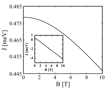
Figure 7: Main panel: Exchange coupling as a function of the magnetic field applied along the wire without the Zeeman effect for $D=20$ nm, $d=l_{z}=30$ nm. Inset: same as main panel but with Zeeman effect.

In general, the influence of the $D$ variation on the exchange energy results from the fact that the two electrons in the 3D QWQD system respond to the variation of a single external parameter by adapting all the variational parameters via the minimization of the system energy. The response varies depending upon the values of other fixed external parameters, which leads to the different decreasing rates observed in Fig. 4(b), for instance.

The in-plane electron confinement can also be enhanced by applying a magnetic field ($B$) along the wire without reducing the wire diameter. As with reducing $D$, $J$ drops with increasing $B$ as seen in Fig. 7, main panel. The drop is nearly linear at large $B$, which is smaller than the drop rate when $D$ approaches $1$ nm [cf. Fig. 4(b)]. This is because the in-plane effective (variational) confinement strength $\omega_{\rho}\approx\sqrt{\Omega_{\rho}^{2}+\omega_{c}^{2}}$ and $\omega_{c}\propto B$, while $\Omega_{\rho}\propto 1/D^{2}$. It should be pointed out that the relatively small $J$ drop in Fig. 7 is obtained in the absence of the Zeeman effect, and it is well known that unlike the small $g$ factor in GaAs ($g\approx-0.44$), InAs QWQD has a much larger $g$ factor ($2$ to $15.5$),Bjork for which the Zeeman effect is dominant over the orbital effect in the $J$ dependence on $B$. For example, the inset of Fig. 7 shows that for $g=8$,gfactor the Zeeman effect totally smears out the orbital effect illustrated in the main panel of Fig. 7, which leads to a negative $J$ for $B>1.1$ T.

Because we model the confinement in the $xy$-plane by a two-dimensional harmonic oscillator potential, the single-particle levels in that plane are given by the Fock-Darwin spectrum, whereby the energy separation between the ground and first excited states decreases as $B$ increases (in contrast, this separation increases with decreasing $D$). In our calculations in Fig. 7, we take $D=20$ nm and $d=l_{z}=30$ nm. At $B=10$ T, the separation is $16.44$ meV, which is considerably larger than the sum of the single-particle energy separation in the $z$-direction ($2.11$ meV) and the Coulomb energy in the triplet state ($1.91$ meV). This observation validates the assumptions of the HL method in which the wavefunctions are taken as linear combination of localized Gaussians separated in the $z$-direction, and only the ground state in the $xy$-plane is taken into account.

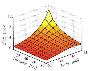
Figure 8: (color online) Addition energy of the second electron $E^{a}(2)$ as a fucntion of wire diameter $D$ and half inter-dot separation $d=l_{z}$.

Experimentally, the measurement of the addition energy is frequently performed to probe the energy levels of the QD.Fasth The addition energy of the $N$-th electron is defined as $E^{a}(N)=\mu(N)-\mu(N-1)$, where $\mu(N)$ is the chemical potential of an $N$-electron QD. Within the VHL method, we are able to calculate the addition energy of the second electron as $E^{a}(2)=\mu(2)-\mu(1)=E^{S}-2e^{0}$, where $E^{S}$ and $e^{0}$ denote the singlet state energy and the single-particle ground state energy, respectively. We plot $E^{a}(2)$ as a function of the geometric parameters $d=l_{z}$ and $D$ in Fig. 8. In general, as the QDs become larger in size (larger $d=l_{z}$ or $D$), the addition energy decreases, for both Coulomb interaction and size quantization effects are reduced. We find (not shown) that at fixed $d=l_{z}$ and $D$, the Coulomb energy between the two electrons are uniformly smaller than $E^{a}(2)$, which is due to the size quantization effects in the coupled QWQDs.

IV Discussions

IV.1 Limitation of the variational Heitler-London method

As an inherent drawback of the HL method, our variational scheme breaks down when the overlap between the localized $s$ states is large, which occurs for small inter-dot separations. For example, in our calculations of the system energies, the VHL method fails for $(d=l_{z})<12$ nm ($0.57r_{0}$) independent of $D$. A signature of the VHL approach breakdown at small $d$ is that the variational parameter $a$ becomes zero in the minimization process. This numerical behavior stems from the fact that at small $d$ a global minimum in the system energies does not exist for the physical range of $a$, given the expression of the variational wavefunction. We note that this shortcoming in the HL method in not apparent in the conventional HL approach. As long as $(d=l_{z})>0$, one can still use the HL method (without variation) to calculate the system energies even though the obtained result is likely to be unphysical.

In Ref. Calderon, , it was pointed out that the HL method breaks down as the quantity $c=\sqrt{\pi/2}(e^{2}/\epsilon a_{B})/\hbar\omega_{0}$ ($a_{B}=\sqrt{\hbar/m\omega_{0}}$) is larger than $1.95$, $2.8$, and $5.8$ for coupled QDs with harmonic oscillator confinement $\hbar\omega_{0}$ in each direction for 1D, 2D and 3D potential models, respectively (this is an extension of the result in Ref. Burkard1, ). We investigate $l_{z}$ from $15$ to $60$ nm, which corresponds to $c$ ranging from $0.44$ to $0.87$, and is uniformly smaller than the smallest breakdown value $c=1.95$. However, as a check of this criterion, we extend our calculation to very large value of $d=l_{z}$ and find that for $D=20$ nm, $J$ becomes very noisy and oscillates randomly for $(d=l_{z})>206$ nm, for which the variational parameter $\hbar\omega_{z}$ is $1.553$ meV, corresponding to $c=1.723$, which is similar to the 1D limit claimed above. However, at this point, $J\sim 10^{-14}$ meV, which bears no practical interest.

IV.2 Comparison with experiments

In recent experiments on InAs QWQDs, $J=2.8$ to $3.2$ meV was reported for a single QD formed in a wire with effective harmonic confinement strength $\hbar\Omega_{z}=6.3$ meV (corresponding to confinement length $2\lambda_{z}=2\sqrt{\hbar/m\Omega_{z}}=46$ nm) and $\hbar\Omega_{\rho}=40$ meV ($2\lambda_{\rho}=2\sqrt{\hbar/m\Omega_{\rho}}=18$ nm).Fasth By fitting these values in our model ($D=18$ nm, $V_{0}=41.6$ meV, $V_{b}=0$ meV, $d=0$ nm and $l_{z}=117.9$ nm), we obtain $J=3.51$ meV, which is comparable to the experimental result.

We note that $J\sim 3$ meV as obtained above is the result for a single QD with potential minimum at $z=0$.footnote2 For double QDs with $D=20$ and $d=l_{z}=30$ nm, we obtain $J\sim 0.5$ meV (Fig. 7), which corresponds to a time scale $(\tau_{J}=\hbar/J)\sim 1.3$ ps, on the same order as the reported spin decoherence time $T_{2}=0.5-1$ ps in InAs QWQDsAEHanson and much smaller than the reported spin dephasing time $T_{2}^{*}=50-500$ ps in self-assembled InAs QDs.MBGroup

V Conclusion

By introducing variational parameters in the HL trial wavefunctions, we achieved lower energies of coupled QWQD system than those calculated by conventional HL method with the relative difference in the tunnel and exchange couplings exceeding $100\%$. As in coupled GaAs QDs based on 2DEG, tunnel and exchange couplings exhibit exponential decay with increasing inter-dot distance or barrier height. Due to the 3D nature of the system, increasing the confinement in the in-plane directions reduces the overlap of the two electrons in the coupling direction (along the wire), which results in the decrease of the exchange coupling. For QDs with different sizes, the addition energy of the second electron is found to be uniformly larger than the two-electron Coulomb interaction because of size quantization effects. By fitting the model potential to experimental parameters, we obtain exchange coupling in agreement with experimental data. Experimental structures based on InAs QWQDs may benefit from the relatively large exchange coupling towards quantum computing applications.

*

Appendix A

The single particle Hamiltonian $\hat{h}$ can be rewritten as

$$\hat{h}=\hat{h}_{L/R}^{0}+W_{L/R},$$ (13)

$$\hat{h}_{L/R}^{0} = \frac{1}{2m}\left({\bf p_{\rho}}+\frac{e}{c}{\bf A}\right)^{2}+\frac{1}{2}{m}\omega_{\rho 0}^{2}{\bm{\rho}}^{2}$$ (14)

$$+\frac{1}{2m}p_{z}^{2}+\frac{1}{2}{m}\omega_{z}^{2}(z\pm a)^{2},$$

$$W_{L/R}=\frac{1}{2}{m}\left(\Omega_{\rho}^{2}-\omega_{\rho 0}^{2}\right){\bm{\rho}}^{2}+V(z)-\frac{1}{2}{m}\omega_{z}^{2}(z\pm a)^{2}.$$ (15)

Since $\hat{h}_{L/R}^{0}\varphi_{L/R}({\bf r})=E_{0}\varphi_{L/R}({\bf r})$ and $E_{0}=\hbar\omega_{\rho}+\hbar\omega_{z}/2$, we only need to calculate the matrix element of $W_{L/R}$. Thus, we have

$$e^{0/1} = \left<\chi_{\pm}\left|\hat{h}\right|\chi_{\pm}\right>$$ (16)

$$= \frac{1}{2}\hbar\omega_{\rho}+\frac{1}{4}\hbar\omega_{z}+\frac{\hbar}{2\omega_{\rho}}\left(\Omega_{\rho}^{2}+\frac{\omega_{c}^{2}}{4}\right)+\frac{1}{1\pm S}\left\{-V_{0}\left(\frac{\hbar}{m\omega_{z}l_{z}^{2}}+1\right)^{-\frac{1}{2}}\exp\left[-\left(\frac{1}{l_{z}^{2}}+\frac{m\omega_{z}}{\hbar}\right)^{-1}\frac{m\omega_{z}}{\hbar l_{z}^{2}}(a+d)^{2}\right]\right.$$

$$-V_{0}\left(\frac{\hbar}{m\omega_{z}l_{z}^{2}}+1\right)^{-\frac{1}{2}}\exp\left[-\left(\frac{1}{l_{z}^{2}}+\frac{m\omega_{z}}{\hbar}\right)^{-1}\frac{m\omega_{z}}{\hbar l_{z}^{2}}(a-d)^{2}\right]$$

$$+V_{b}\left(\frac{\hbar}{m\omega_{z}l_{bz}^{2}}+1\right)^{-\frac{1}{2}}\exp\left[-\left(\frac{1}{l_{bz}^{2}}+\frac{m\omega_{z}}{\hbar}\right)^{-1}\frac{m\omega_{z}}{\hbar l_{bz}^{2}}a^{2}\right]\mp 2SV_{0}\left(\frac{\hbar}{m\omega_{z}l_{z}^{2}}+1\right)^{-\frac{1}{2}}\exp\left[-\left(\frac{1}{l_{z}^{2}}+\frac{m\omega_{z}}{\hbar}\right)^{-1}\frac{m\omega_{z}}{\hbar l_{z}^{2}}d^{2}\right]$$

$$\pm\left.SV_{b}\left(\frac{\hbar}{m\omega_{z}l_{bz}^{2}}+1\right)^{-\frac{1}{2}}\mp\frac{S}{2}m\omega_{z}^{2}a^{2}\right\}.$$

In above, $S=\int d{\bf r}\varphi_{L}^{*}({\bf r})\varphi_{R}({\bf r})=\exp\left(-m\omega_{z}a^{2}/\hbar\right)$ is the overlap between the two localized $s$ states.

The singlet and triplet energies are evaluated in a similar fashion and the results are:

$$E^{S/T} = \left<\Psi_{\pm}\left|\hat{H}_{orb}\right|\Psi_{\pm}\right>$$ (17)

$$= 2E_{0}+\frac{1}{1\pm S^{2}}\left[\left<\varphi_{L}\varphi_{R}|W_{1}+W_{2}+W_{3}+C|\varphi_{L}\varphi_{R}\right>\right.\pm\left.Re\left<\varphi_{L}\varphi_{R}|W_{1}+W_{2}+W_{3}+C|\varphi_{R}\varphi_{L}\right>\right],$$

$$\left<\varphi_{L}\varphi_{R}\left|W_{1}\right|\varphi_{L}\varphi_{R}\right> = \left<\varphi_{L}\varphi_{R}\left|V(z_{1})+V(z_{2})\right|\varphi_{L}\varphi_{R}\right>$$ (18)

$$= -2V_{0}\left(\frac{\hbar}{m\omega_{z}l_{z}^{2}}+1\right)^{-\frac{1}{2}}\left\{\exp\left[-\left(\frac{1}{l_{z}^{2}}+\frac{m\omega_{z}}{\hbar}\right)^{-1}\frac{m\omega_{z}}{\hbar l_{z}^{2}}(a+d)^{2}\right]\right.$$

$$+\left.\exp\left[-(\frac{1}{l_{z}^{2}}+\frac{m\omega_{z}}{\hbar})^{-1}\frac{m\omega_{z}}{\hbar l_{z}^{2}}(a-d)^{2}\right]\right\}$$

$$+2V_{b}\left(\frac{\hbar}{m\omega_{z}l_{bz}^{2}}+1\right)^{-\frac{1}{2}}\exp\left[-\left(\frac{1}{l_{bz}^{2}}+\frac{m\omega_{z}}{\hbar}\right)^{-1}\frac{m\omega_{z}}{\hbar l_{bz}^{2}}a^{2}\right],$$

$$\left<\varphi_{L}\varphi_{R}\left|W_{1}\right|\varphi_{R}\varphi_{L}\right> = \left<\varphi_{L}\varphi_{R}\left|V(z_{1})+V(z_{2})\right|\varphi_{R}\varphi_{L}\right>$$ (19)

$$= 2\exp\left(-2\frac{m\omega_{z}}{\hbar}a^{2}\right)\left\{-2V_{0}\left(\frac{\hbar}{m\omega_{z}l_{z}^{2}}+1\right)^{-\frac{1}{2}}\exp\left[-\left(\frac{1}{l_{z}^{2}}+\frac{m\omega_{z}}{\hbar}\right)^{-1}\frac{m\omega_{z}}{\hbar l_{z}^{2}}d^{2}\right]\right.$$

$$+\left.V_{b}\left[\frac{\hbar}{m\omega_{z}l_{bz}^{2}}+1\right]^{-\frac{1}{2}}\right\},$$

$$\left<\varphi_{L}\varphi_{R}\left|W_{2}\right|\varphi_{L}\varphi_{R}\right> = \left<\varphi_{L}\varphi_{R}\left|-\frac{1}{2}{m}\omega_{z}^{2}(z_{1}+a)^{2}-\frac{1}{2}{m}\omega_{z}^{2}(z_{2}-a)^{2}\right|\varphi_{L}\varphi_{R}\right>$$ (20)

$$= -\frac{1}{2}\hbar\omega_{z},$$

$$\left<\varphi_{L}\varphi_{R}\left|W_{2}\right|\varphi_{R}\varphi_{L}\right> = \left<\varphi_{L}\varphi_{R}\left|-\frac{1}{2}{m}\omega_{z}^{2}(z_{1}+a)^{2}-\frac{1}{2}{m}\omega_{z}^{2}(z_{2}-a)^{2}\right|\varphi_{R}\varphi_{L}\right>$$ (21)

$$= -m\omega_{z}^{2}\left(\frac{\hbar}{2m\omega_{z}}+a^{2}\right)\exp\left(-2\frac{m\omega_{z}}{\hbar}a^{2}\right),$$

$$\left<\varphi_{L}\varphi_{R}\left|W_{3}\right|\varphi_{L}\varphi_{R}\right> = \left<\varphi_{L}\varphi_{R}\left|\frac{1}{2}{m}\left(\Omega_{\rho}^{2}-\omega_{\rho 0}^{2}\right)\left({\bm{\rho}}_{1}^{2}+{\bm{\rho}}_{2}^{2}\right)\right|\varphi_{L}\varphi_{R}\right>$$ (22)

$$=\frac{\hbar}{\omega_{\rho}}\left(\Omega_{\rho}^{2}+\frac{\omega_{c}^{2}}{4}-\omega_{\rho}^{2}\right),$$

$$\left<\varphi_{L}\varphi_{R}\left|W_{3}\right|\varphi_{R}\varphi_{L}\right> = \left<\varphi_{L}\varphi_{R}\left|\frac{1}{2}{m}\left(\Omega_{\rho}^{2}-\omega_{\rho 0}^{2}\right)\left({\bm{\rho}}_{1}^{2}+{\bm{\rho}}_{2}^{2}\right)\right|\varphi_{R}\varphi_{L}\right>$$ (23)

$$= \frac{\hbar}{\omega_{\rho}}\left(\Omega_{\rho}^{2}+\frac{\omega_{c}^{2}}{4}-\omega_{\rho}^{2}\right)\exp\left(-2\frac{m\omega_{z}}{\hbar}a^{2}\right).$$

The Coulomb matrix elements in Eq. (9) are given by

$$\left<\varphi_{L}\varphi_{R}\left|C\right|\varphi_{L}\varphi_{R}\right> = \left<\varphi_{L}\varphi_{R}\left|\frac{e^{2}}{\epsilon\left|{\bf r_{1}}-{\bf r_{2}}\right|}\right|\varphi_{L}\varphi_{R}\right>$$ (24)

$$=\frac{e^{2}}{\epsilon}\left(\frac{2m\omega_{z}}{\pi\hbar}\right)^{\frac{1}{2}}\int_{0}^{1}\frac{1}{1+\left(\frac{\omega_{z}}{\omega_{\rho}}-1\right)t^{2}}\exp\left(-2\frac{m\omega_{z}}{\hbar}a^{2}t^{2}\right)dt,$$

$$\left<\varphi_{L}\varphi_{R}\left|C\right|\varphi_{R}\varphi_{L}\right> = \left<\varphi_{L}\varphi_{R}\left|\frac{e^{2}}{\epsilon\left|{\bf r_{1}}-{\bf r_{2}}\right|}\right|\varphi_{R}\varphi_{L}\right>$$ (30)

$$=\frac{e^{2}}{\epsilon}\left(\frac{2m\omega_{z}}{\pi\hbar}\right)^{\frac{1}{2}}\exp\left(-2\frac{m\omega_{z}}{\hbar}a^{2}\right)\int_{0}^{1}\frac{1}{1+\left(\frac{\omega_{z}}{\omega_{\rho}}-1\right)t^{2}}dt$$

$$=\frac{e^{2}}{\epsilon}\left(\frac{2m\omega_{z}}{\pi\hbar}\right)^{\frac{1}{2}}\exp\left(-2\frac{m\omega_{z}}{\hbar}a^{2}\right)\times\left\{\begin{array}[]{lcl}{\left(1-\frac{\omega_{z}}{\omega_{\rho}}\right)^{-\frac{1}{2}}\text{arctanh}\left[\left(1-\frac{\omega_{z}}{\omega_{\rho}}\right)^{\frac{1}{2}}\right]}&\mbox{for}&\omega_{z}<\omega_{\rho}\\ \\ {\left(\frac{\omega_{z}}{\omega_{\rho}}-1\right)^{-\frac{1}{2}}\arctan\left[\left(\frac{\omega_{z}}{\omega_{\rho}}-1\right)^{\frac{1}{2}}\right]}&\mbox{for}&\omega_{z}>\omega_{\rho}\\ \\ 1&\mbox{for}&\omega_{z}=\omega_{\rho}.\end{array}\right.$$

Practically, the one dimensional integrals in Eqs. (A.12) and (LABEL:eqn:Coulomb_D_2)] are numerically evaluated using adaptive quadratures. We note that in the 1D limit ($\omega_{\rho}\rightarrow\infty$), the integrals have logarithmic divergence,Calderon while they both approach zero in the oppsite limit ($\omega_{\rho}\rightarrow 0$). For $\omega_{\rho}=\omega_{z}=\omega_{0}$, the integrals in Eqs. (A.12) and (LABEL:eqn:Coulomb_D_2) simplify to $[e^{2}/(2a\epsilon)]\text{Erf}(a\sqrt{2m\omega_{0}/\hbar})$ and $(e^{2}/\epsilon)\sqrt{2m\omega_{0}/(\pi\hbar)})\exp(-2m\omega_{0}a^{2}/\hbar)$, respectively. These results are identical to the results in Ref. Calderon, , where the Coulomb matrix elements were calculated between coupled spherically symmetric Gaussian trial wavefunctions.

References

- (1) C. Fasth, A. Fuhrer, M. T. Björk, and L. Samuelson, Nano. Lett. 5, 1487 (2005); A. Fuhrer, C. Fasth, and L. Samuelson, Appl. Phys. Lett. 91, 052109 (2007).
- (2) M. T. Björk, A. Fuhrer, A. E. Hansen, M. W. Larsson, L. E. Fröberg, and L. Samuelson, Phys. Rev. B 72, 201307(R) (2005).
- (3) C. Fasth, A. Fuhrer, L. Samuelson, V. N. Golovach, and D. Loss, Phys. Rev. Lett. 98, 266801 (2007).
- (4) J. R. Petta, A.C. Johnson, J. M. Taylor, E. A. Laird, A. Yacoby, M. D. Lukin, C. M. Marcus, M. P. Hanson, and A. C. Gossard, Science 309, 2180 (2005).
- (5) J. M. Elzerman, R. Hanson, J. S. Greidanus, L. H. Willems van Beveren, S. De Franceschi, L. M. Vandersypen, S. Tarucha, and L. P. Kouwenhoven, Phys. Rev. B 67, 161308(R) (2003).
- (6) T. Hatano, M. Stopa, and S. Tarucha, Science 309, 268 (2005).
- (7) M. Pi, A. Emperador, M. Barranco, F. Garcias, K. Muraki, S. Tarucha, and D. G. Austing, Phys. Rev. Lett., 87, 066801 (2001).
- (8) D. Bellucci, M. Rontani, F. Troiani, G. Goldoni, and E. Molinari, Phys. Rev. B 69, 201308(R) (2004).
- (9) G. Burkard, D. Loss, and D. P. DiVincenzo, Phys. Rev. B 59, 2070 (1999).
- (10) X. Hu and S. Das Sarma, Phys. Rev. A 61, 062301 (2000).
- (11) D. V. Melnikov, J.-P. Leburton, A. Taha, and N. Sobh, Phys. Rev. B 74, 041309 (2006).
- (12) A. Harju, S. Siljamäki, and R. M. Nieminen, Phys. Rev. Lett. 88, 226804 (2002).
- (13) B. Szafran, F. M. Peeters, and S. Bednarek, Phys. Rev. B 70, 205318 (2004).
- (14) W. Dybalski and P. Hawrylak, Phys. Rev. B 72, 205432 (2005).
- (15) L.-X. Zhang, P. Matagne, J.-P. Leburton, R. Hanson, and L. P. Kouwenhoven, Phys. Rev. B 69, 245301 (2004).
- (16) L.-X. Zhang, D. V. Melnikov, and J.-P. Leburton, Phys. Rev. B 74, 205306 (2006).
- (17) M. Stopa and C. M. Marcus, cond-mat/0604008 (2006).
- (18) M. J. Calderón, B. Koiller, and S. Das Sarma, Phys. Rev. B 74 , 045310 (2006).
- (19) G. Burkard, G. Seelig, and D. Loss, Phys. Rev. B 62, 2581 (2000).
- (20) B. Koiller, R. B. Capaz, X. Hu, and S. Das Sarma, Phys. Rev. B 70, 115207 (2004).
- (21) A. E. Hansen, M. T. Björk, C. Fasth, C. Thelander, and L. Samuelson, Phys. Rev. B 71, 205328 (2005).
- (22) An intial guess for the variational parameters is given near their nominal values and then we use the fminsearch subroutine in MATLAB which employs the Nelder-Mead simplex method to search for the minima of the system energies with respect to these parameters. It turns out that unless the overlap between the localized states is too large, the simplex method always finds a global minimum within the physically reasonable range of the variational parameters.
- (23) R. de Sousa, X. Hu, and S. Das Sarma, Phys. Rev. A 64, 042307 (2001).
- (24) We take measured in QDs with similar geometry,Fasth although the linear dependence of on magnetic field is clear even for .
- (25) Recently, the VHL method has been applied to calculate the two-electron energies in a single two-dimensional elliptical QD. By comparing the results to numerical exact diagonalization results, it is shown that the VHL method is successful in reproducing the magnetic field dependence of .Agarwal
- (26) I. A. Merkulov, Al. L. Efros, and M. Rosen, Phys. Rev. B. 65, 205309 (2002); P.-F. Braun, X. Marie, L. Lombez, B. Urbaszek, T. Amand, P. Renucci, V. K. Kalevich, K. V. Kavokin, O. Krebs, P. Voisin, and Y. Masumoto, Phys. Rev. Lett. 94 116601 (2005).
- (27) S. Agarwal, D. V. Melnikov, L.-X. Zhang, and J. P. Leburton (unpublished).