Strange quark contribution to nucleon form factors

Abstract:

We discuss methods for the calculation of disconnected diagrams and their application to various form factors of the nucleon. In particular, we present preliminary results for the strange contribution to the scalar and axial form factors, calculated with $N_{f}=2$ dynamical flavors of Wilson fermions on an anisotropic lattice.

1 Introduction

In recent years, there has been a great deal of progress in probing the structure of the nucleon on the lattice. With few exceptions, however, such studies have been restricted to the calculation of isovector quantities or otherwise neglect the contribution of “disconnected diagrams,” due to the large cost associated with their calculation. The full inclusion of such contributions is necessary, however, to complete the picture of the nucleon, and with new methods and the computational resources now available, it appears that the time may be ripe to do so.

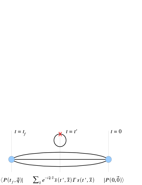
Figure 1: Schematic representation of a disconnected diagram, giving a strange form factor of the proton. Here $\Gamma$ is the appropriate gamma insertion for the form factor of interest.

In this contribution, we focus on a family of observables whose matrix elements are inherently disconnected, the strange quark contribution to the elastic form factors of the nucleon. Such a matrix element is shown schematically in Fig. 1; by “disconnected,” we mean that the diagram includes an insertion on a quark loop that is coupled to the baryon correlator only via the gauge field. This requires the calculation of a trace of the quark propagator over spin, color, and spatial indices. Since an exact calculation would require a number of inversions proportional to the lattice volume, the trace is generally estimated stochastically, which introduces a new source of statistical error whose reduction is discussed in section 2. In particular, we propose a novel method for variance reduction based on the subtraction of the coarse-grid operator as defined in an adaptive multigrid scheme.

The strange contribution to the electromagnetic and axial form factors, $G^{s}_{E}(Q^{2})$, $G^{s}_{M}(Q^{2})$, and $G^{s}_{A}(Q^{2})$, are the subject of much experimental interest but remain poorly determined to date. For a review and recent determination, see Ref. [1]. The scalar form factor, $G^{s}_{S}(Q^{2})$, is not directly accessible to experiment, but nevertheless plays an important role in models of nucleon structure. Several lattice calculations of these quantities have been attempted, primarily in the quenched approximation and with varying degrees of success (see, for example, Ref. [2, 3, 4, 5, 6, 7, 8, 9, 10]). In this contribution, we discuss the outlook for a calculation of the strange form factors on large, unquenched, anisotropic lattices. We also present preliminary results from an exploratory calculation of the axial and scalar form factors at $Q^{2}=0$.

The paper is organized as follows. In section 2, we discuss general considerations for calculating the trace and describe the particular approach employed in our exploratory calculation. We also outline a multigrid method for variance reduction. In section 3, we discuss our approach for extracting the form factors from the corresponding matrix elements. Finally, in section 4 we present preliminary results for $G^{s}_{A}(Q^{2}=0)$ and $G^{s}_{S}(Q^{2}=0)$.

2 Trace estimation

2.1 Noisy estimators and dilution

The standard method for estimating the trace relies on calculating the inverse against a set of noise vectors $\eta$ whose components are random elements of $U(1)$ or $Z_{2}$ [11], as follows:

$$\mathrm{Tr}(\Gamma D^{-1})\approx\frac{1}{N}\sum_{i=1}^{N}\eta_{i}^{\dagger}\Gamma D^{-1}\eta_{i},\quad\langle\eta_{(x)}^{\dagger}\eta_{(y)}\rangle=\delta_{x,y}\,.$$ (1)

Given a finite ensemble of such noisy sources, this procedure introduces a new source of statistical error due to the off-diagonal terms that do not cancel exactly. Since the fall-off of the quark propagator is exponential, this error is dominated by the “near off-diagonals,” terms that connect points local in space (we treat the sum over color and spin exactly). It follows that one may greatly reduce this error via dilution, i.e. by dividing the stochastic source into subsets and inverting on these separately [12]. For example, with simple even/odd dilution,

$$\mathrm{Tr}(\Gamma D^{-1})\approx\frac{1}{N}\sum_{i=1}^{N}\eta_{i}^{(e)\dagger}\Gamma D^{-1}\eta_{i}^{(e)}+\frac{1}{N}\sum_{i=1}^{N}\eta_{i}^{(o)\dagger}\Gamma D^{-1}\eta_{i}^{(o)}\,.$$ (2)

Here $\eta_{i}^{(e)}$ and $\eta_{i}^{(o)}$ are non-zero only on the even and odd sites, respectively, and $\eta_{i}^{(e)}+\eta_{i}^{(o)}=\eta_{i}$ gives the original noise vector.

In a full calculation, one faces two sources of error: the usual gauge noise and the error in the trace. As a baseline in our exploratory calculation, we largely eliminate the second source of error by calculating a “nearly exact” trace on each of four time-slices. This is accomplished by employing a large number of sources ($1024\times 12$ for color/spin) where each source is nonzero on only four sites on each of the four time-slices. The sites are chosen such that the smallest spatial separation between them is $8\sqrt{2}a_{s}$. Any residual contamination, which we observe to be small, is gauge-variant and averages to zero. As an aside, we note that this approach is equivalent to using a single noise vector (or more precisely, a set of three vectors over space and color that are mutually orthogonal in color) together with “extreme dilution.”

2.2 Multigrid variance reduction

A number of methods have been proposed to reduce “far off-diagonal” contributions to the variance in estimates of the trace (e.g. Ref. [13] in these proceedings). Such contributions become increasingly important if we are to consider light quarks. A particularly promising approach is to calculate the trace exactly in the subspace spanned by the lowest eigenmodes of the Dirac operator [14] and estimate the remaining piece stochastically [15]. In addition to reducing the variance, this method has the advantage that the set of eigenvectors, once calculated, may also be used to precondition the inverter and speed up the large number of inversions needed for the remaining piece.

Recently, an adaptive geometric multigrid algorithm was shown to greatly reduce critical slowing down in the two-dimensional U(1) Schwinger model [16] (see also Ref. [17] in these proceedings). The method generalizes straightforwardly to four dimensions, and like eigenvector projection, it is most advantageous when the set-up cost may be amortized over a large number of inversions, as is typical for disconnected diagrams. (The methods proposed in Refs. [18, 19, 20] have similar advantages.) Even more promising for this application, however, is the possibility of greatly reducing the variance in stochastic estimates of the trace by first subtracting the inverse calculated on the coarse level. Following Ref. [16], we define a coarse approximation $\tilde{A}=P^{\dagger}AP$ to the positive definite operator $A=D^{\dagger}D$, where $P$ is the prolongator that takes vectors from the coarse to the fine grid and $P^{\dagger}$ is the corresponding restriction operator. The inverse $\tilde{A}^{-1}$ can be calculated inexpensively, and hence the operator $P\tilde{A}^{-1}P^{\dagger}$ can be used in an approximation to the full trace, i.e. $\mathrm{Tr}(\Gamma D^{-1})\approx\mathrm{Tr}(\Gamma P\tilde{A}^{-1}P^{\dagger}D^{\dagger})$. Employing the cyclic property of the trace, we have $\mathrm{Tr}(\Gamma P\tilde{A}^{-1}P^{\dagger}D^{\dagger})=\mathrm{Tr}(\tilde{A}^{-1}P^{\dagger}D^{\dagger}\Gamma P)$. This is now the trace of an operator on the coarse grid, which can be determined at a much smaller cost, either stochastically or exactly. At the same time, it captures the long-range physics and should give a very good estimate of the full trace. For an unbiased estimate, we require the residual contribution on the fine grid, but this contribution is expected to be small and may be estimated with a smaller number of (possibly diluted) noise vectors, $N$, without significantly affecting the variance. An unbiased estimate of the full trace is thus given by

$$\mathrm{Tr}(\Gamma D^{-1})\approx\frac{1}{N}\sum_{i=1}^{N}\eta_{i}^{\dagger}\left[\Gamma D^{-1}-\Gamma P\tilde{A}^{-1}P^{\dagger}D^{\dagger}\right]\eta_{i}+\frac{1}{\tilde{N}}\sum_{i=1}^{\tilde{N}}\tilde{\eta}^{\dagger}_{i}\left[\tilde{A}^{-1}P^{\dagger}D^{\dagger}\Gamma P\right]\tilde{\eta}_{i}\,.$$ (3)

Here $\tilde{N}$ is the number of noise vectors $\tilde{\eta}$ on the coarse grid. We note, however, that given the large reduction in degrees of freedom, it will often be practical to calculate the second term exactly.

The multigrid method of Ref. [16] may be generalized to work with the Dirac operator $D$ directly, rather than $A=D^{\dagger}D$. In this case the restriction operator is no longer the conjugate of the prolongation operator, but the basic variance reduction method goes through as before. Work is underway to apply this method as a post-processing step to the results reported below.

3 Extracting form factors

Given an estimate of the trace on each of an ensemble of configurations, the next step is to correlate these with the proton correlator to calculate the form factors. A number of methods exist for doing so. Those that have been used to date rely on having an estimate of the trace on many adjacent time-slices. In the most basic approach, the trace is calculated over the entire lattice, and the form factor is extracted from the time-dependence of the proton correlator, correlated with this background. Here we take a more direct approach by inserting the quark loop on a single time-slice, labeled by $t^{\prime}$, at the midpoint of the proton correlator (see Fig. 1). The source and sink are moved apart symmetrically, with $t_{f}-t^{\prime}=t^{\prime}-t_{0}$, and we look for a plateau at large separations. More concretely, for the axial form factor at $Q^{2}=0$, we calculate

$$R_{A}(t,t^{\prime},t_{0}) = \frac{1}{3}\sum_{i=1}^{3}\frac{\sum_{\vec{x},\vec{x}^{\prime}}[(1+\gamma_{4})\gamma_{i}\gamma_{5}]^{\alpha\beta}[\langle P^{\beta}(\vec{x},t)A_{i}(\vec{x}^{\prime},t^{\prime})\bar{P}^{\alpha}(\vec{0},t_{0})\rangle-\langle P^{\beta}(\vec{x},t)\bar{P}^{\alpha}(\vec{0},t_{0})\rangle\langle A_{i}(\vec{x}^{\prime},t^{\prime})\rangle]}{\sum_{\vec{x}}(1+\gamma_{4})^{\alpha\beta}\langle P^{\beta}(\vec{x},t)\bar{P}^{\alpha}(\vec{0},t_{0})\rangle}$$ (4)

$$\rightarrow G_{A}^{s}(Q^{2}=0)\ \ \mathrm{for}\ \ (t-t^{\prime})=(t^{\prime}-t_{0})\ \mathrm{large.}$$

Because the expectation value of the axial current vanishes, the subtraction of the second term is not formally required, but it may serve to cancel contributions to the error. For the scalar form factor, the subtraction of the nonvanishing condensate is necessary, and we have

$$R_{S}(t,t^{\prime},t_{0}) = \frac{\sum_{\vec{x},\vec{x}^{\prime}}(1+\gamma_{4})^{\alpha\beta}\langle P^{\beta}(\vec{x},t)[\bar{\psi}\psi(\vec{x}^{\prime},t^{\prime})]\bar{P}^{\alpha}(\vec{0},t_{0})\rangle}{\sum_{\vec{x}}(1+\gamma_{4})^{\alpha\beta}\langle P^{\beta}(\vec{x},t)\bar{P}^{\alpha}(\vec{0},t_{0})\rangle}-\sum_{\vec{x}^{\prime}}\langle\bar{\psi}\psi(\vec{x}^{\prime},t^{\prime})\rangle$$ (5)

$$\rightarrow G_{S}^{s}(Q^{2}=0)\ \ \mathrm{for}\ \ (t-t^{\prime})=(t^{\prime}-t_{0})\ \mathrm{large.}$$

It is important to note that if one has found the trace on multiple time-slices, this information is not wasted, since one can repeat the measurement with the system centered at various points in the lattice and thereby increase the statistics. For the results presented below, we have employed four evenly-spaced timeslices.

4 Preliminary results

At present, we are preparing to calculate disconnected diagrams on large anisotropic lattices with $N_{f}=2+1$ dynamical flavors of clover-improved Wilson fermions. These lattices are being generated by members of the Lattice Hadron Physics Collaboration (LHPC) for the purpose of studying excited-state spectroscopy (see, e.g., Ref. [21] in these proceedings). Significant effort is being invested to construct improved variational sources for the nucleon on these lattices, and we plan to utilize these to improve the signal for the disconnected form factors.

In preparation for this calculation, we have performed an exploratory study on a smaller plain-Wilson test lattice of size $16^{3}\times 64$ with two dynamical flavors and $M_{\pi}\approx 360$ MeV. The lattice is anisotropic with $a_{s}=0.118(2)\ \mathrm{fm}\approx 3a_{t}$, and we have analyzed 351 independent configurations. Proton correlators were calculated with gaussian smearing at source and sink, and we find that the ground state is isolated near $t=10a$.

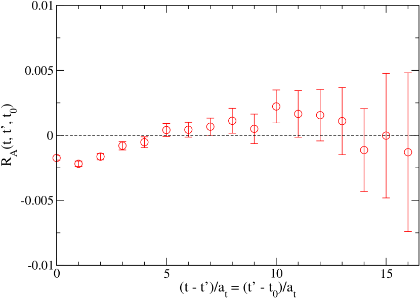
Figure 2: Results for axial form factor, with $R_{A}$ as defined in the text.

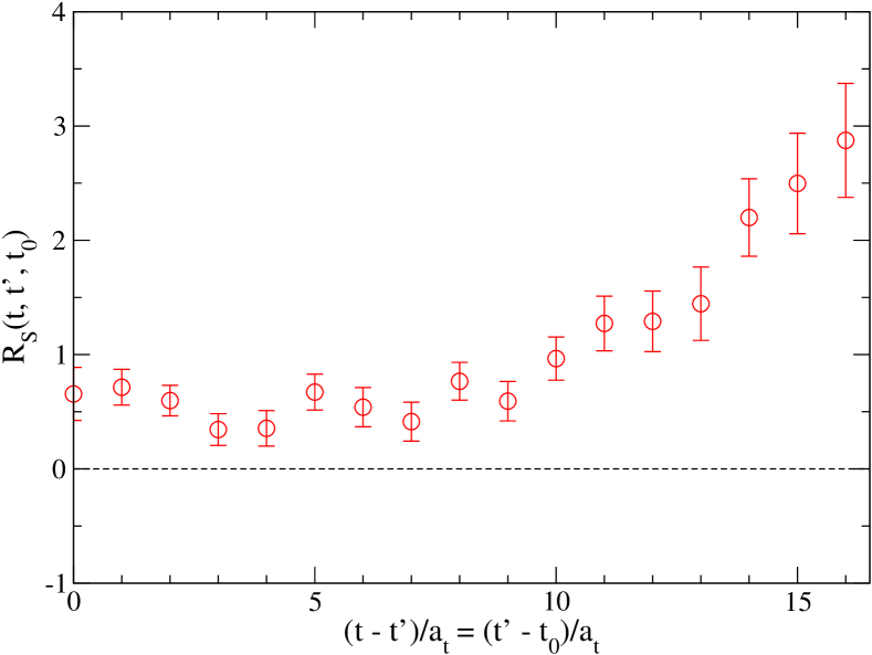
Figure 3: Results for scalar form factor, with $R_{S}$ as defined in the text.

Fig. 3 shows our preliminary results for the strange contribution to the axial form factor, as defined in Eq. (4). Errors have been calculated via jackknife. We observe significant correlation at small time separations, but for $t>5a_{t}$ the results are consistent with zero. Our analysis is still in progress, but it appears that it may only be possible to set a limit, given the statistics available for this ensemble. The rapid disappearance of the signal serves as a strong argument for the importance of better extended sources for the nucleon.

The prospects for the scalar form factor are more promising, as shown in Fig. 3. Here the signal persists for all time separations. The increase at large times is anomalous and possibly represents a finite size effect, since at $(t-t^{\prime})=16a_{t}$ the proton correlator extends halfway across the lattice.

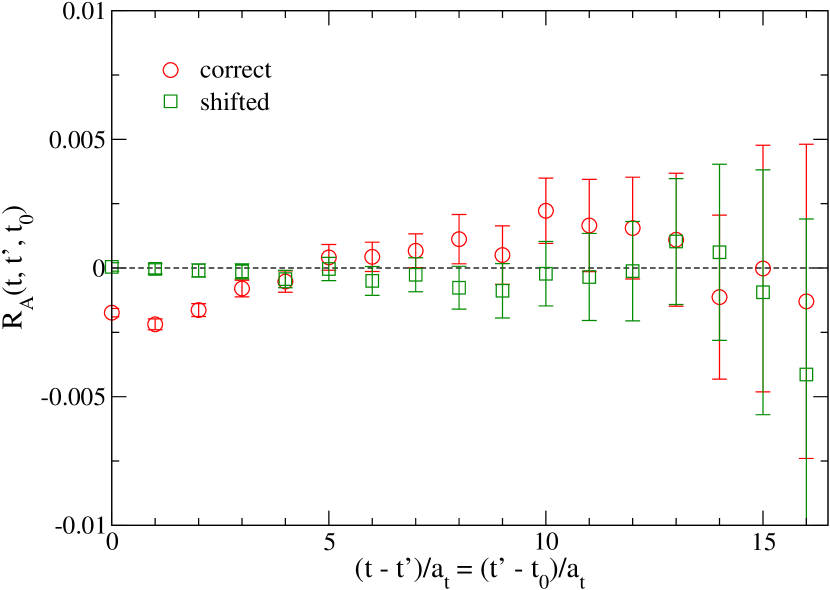
Figure 4: Confirmation of correlation in axial channel.

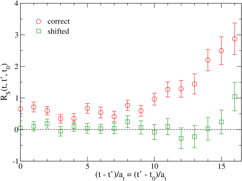
Figure 5: Confirmation of correlation in scalar channel.

As shown by these and past results, the evaluation of disconnected diagrams remains a very challenging problem. Schematically, we are calculating a correlation (cf. Eq. (4),(5)),

$$\frac{\langle\mathrm{nucleon}\times\mathrm{trace}\rangle-\langle\mathrm{nucleon}\rangle\langle\mathrm{trace}\rangle}{\langle\mathrm{nucleon}\rangle}\,,$$ (6)

that is observed to be small compared to the characteristic fluctuations in the trace and nucleon correlator. As a “sanity check,” we confirm that our signal is genuine by shifting configurations and purposely correlating the nucleon on the $i$th configuration with the trace on the $(i+s)$th. As shown in Figs. 5 and 5, the signal vanishes as expected.

5 Conclusions

Disconnected diagrams represent a considerable challenge for the lattice, but they are central to a wide range of physical problems. Among these is the strange quark contribution to form factors of the nucleon. By applying both new and established techniques, we hope to obtain accurate, unquenched determinations of these quantities. Preliminary results are encouraging, and should only improve with increased statistics, better interpolating operators for the nucleon, and the implementation of multigrid variance reduction.

- [1] S. Pate, Strange Nucleon Form Factors from and Elastic Scattering, arXiv:0704.1115.
- [2] M. Fukugita, Y. Kuramashi, M. Okawa, and A. Ukawa, Proton spin structure from lattice QCD, Phys. Rev. Lett. 75 (1995) 2092–2095 [hep-lat/9501010].
- [3] M. Fukugita, Y. Kuramashi, M. Okawa, and A. Ukawa, Pion - nucleon sigma term in lattice QCD, Phys. Rev. D51 (1995) 5319–5322 [hep-lat/9408002].
- [4] S. J. Dong, J. F. Lagaë, and K. F. Liu, Flavor singlet g(A) from lattice QCD, Phys. Rev. Lett. 75 (1995) 2096–2099 [hep-ph/9502334].
- [5] S. J. Dong, J. F. Lagaë, and K. F. Liu, Term , in Nucleon, and Scalar Form Factor — a Lattice Study, Phys. Rev. D54 (1996) 5496–5500 [hep-ph/9602259].
- [6] S. J. Dong, K. F. Liu, and A. G. Williams, Lattice calculation of the strangeness magnetic moment of the nucleon, Phys. Rev. D58 (1998) 074504 [hep-ph/9712483].
- [7] TXL Collaboration, S. Güsken et al., The pion nucleon sigma-term with dynamical Wilson fermions, Phys. Rev. D59 (1999) 054504 [hep-lat/9809066].
- [8] TXL Collaboration, S. Güsken et al., Flavor singlet axial vector coupling of the proton with dynamical Wilson fermions, Phys. Rev. D59 (1999) 114502.
- [9] Kentucky Field Theory Collaboration, N. Mathur and S.-J. Dong, Strange magnetic moment of the nucleon from lattice QCD, Nucl. Phys. Proc. Suppl. 94 (2001) 311–314 [hep-lat/0011015].
- [10] R. Lewis, W. Wilcox, and R. M. Woloshyn, The nucleon’s strange electromagnetic and scalar matrix elements, Phys. Rev. D67 (2003) 013003 [hep-ph/0210064].
- [11] S.-J. Dong and K.-F. Liu, Stochastic estimation with Z(2) noise, Phys. Lett. B328 (1994) 130–136.
- [12] J. Foley et al., Practical all-to-all propagators for lattice QCD, Comput. Phys. Commun. 172 (2005) 145–162 [hep-lat/0505023].
- [13] S. Collins, G. Bali, and A. Schäfer, Disconnected contributions to hadronic structure: a new method for stochastic noise reduction, PoS LATTICE 2007 (2007) 141 [arXiv:0709.3217].
- [14] H. Neff, N. Eicker, T. Lippert, J. W. Negele, and K. Schilling, On the low fermionic eigenmode dominance in QCD on the lattice, Phys. Rev. D64 (2001) 114509 [hep-lat/0106016].
- [15] SESAM Collaboration, G. S. Bali, H. Neff, T. Duessel, T. Lippert, and K. Schilling, Observation of string breaking in QCD, Phys. Rev. D71 (2005) 114513 [hep-lat/0505012].
- [16] J. Brannick, R. C. Brower, M. A. Clark, J. C. Osborn, and C. Rebbi, Adaptive Multigrid Algorithm for Lattice QCD, arXiv:0707.4018.
- [17] J. Brannick, R. C. Brower, M. A. Clark, J. C. Osborn, and C. Rebbi, Adaptive multigrid algorithm for the QCD Dirac-Wilson operator, PoS LATTICE 2007 (2007) 029.
- [18] M. Lüscher, Local coherence and deflation of the low quark modes in lattice QCD, JHEP 07 (2007) 081 [arXiv:0706.2298].
- [19] A. Stathopoulos and K. Orginos, Computing and deflating eigenvalues while solving multiple right hand side linear systems in Quantum Chromodynamics, arXiv:0707.0131.
- [20] R. B. Morgan and W. Wilcox, Deflated Iterative Methods for Linear Equations with Multiple Right-Hand Sides, arXiv:0707.0505.
- [21] H.-W. Lin, R. G. Edwards, and B. Joó, Parameter Tuning of Three-Flavor Dynamical Anisotropic Clover Action, PoS LATTICE 2007 (2007) 119 [arXiv:0709.4680].